
94% of researchers rate our articles as excellent or good
Learn more about the work of our research integrity team to safeguard the quality of each article we publish.
Find out more
ORIGINAL RESEARCH article
Front. Remote Sens., 30 August 2023
Sec. Image Analysis and Classification
Volume 4 - 2023 | https://doi.org/10.3389/frsen.2023.1221757
 Kadio S. R. Aka1,2*
 Semihinva Akpavi3N’Da Hyppolite Dibi4,5
 Amos T. Kabo-Bah6
 Amatus Gyilbag7
 Edward Boamah8
Land use and land cover (LULC) changes are one of the main factors contributing to ecosystem degradation and global climate change. This study used the Gontougo Region as a study area, which is fast changing in land occupation and most vulnerable to climate change. The machine learning (ML) method through Google Earth Engine (GEE) is a widely used technique for the spatiotemporal evaluation of LULC changes and their effects on land surface temperature (LST). Using Landsat 8 OLI and TIRS images from 2015 to 2022, we analyzed vegetation cover using the Normalized Difference Vegetation Index (NDVI) and computed LST. Their correlation was significant, and the Pearson correlation (r) was negative for each correlation over the year. The correspondence of the NDVI and LST reclassifications has also shown that non-vegetation land corresponds to very high temperatures (34.33°C–45.22°C in 2015 and 34.26°C–45.81°C in 2022) and that high vegetation land corresponds to low temperatures (17.33°C–28.77°C in 2015 and 16.53 29.11°C in 2022). Moreover, using a random forest algorithm (RFA) and Sentinel-2 images for 2015 and 2022, we obtained six LULC classes: bareland and settlement, forest, waterbody, savannah, annual crops, and perennial crops. The overall accuracy (OA) of each LULC map was 93.77% and 96.01%, respectively. Similarly, the kappa was 0.87 in 2015 and 0.92 in 2022. The LULC classes forest and annual crops lost 48.13% and 65.14%, respectively, of their areas for the benefit of perennial crops from 2015 to 2022. The correlation between LULC and LST showed that the forest class registered the low mean temperature (28.69°C in 2015 and 28.46°C in 2022), and the bareland/settlement registered the highest mean temperature (35.18°C in 2015 and 35.41°C in 2022). The results show that high-resolution images can be used for monitoring biophysical parameters in vegetation and surface temperature and showed benefits for evaluating food security.
The sixth report of the Intergovernmental Panel on Climate Change (IPCC) reveals that most of the observed increase in global average temperature since the middle of the 20th century most likely results from the observed increase in anthropogenic greenhouse gas (GHG) concentrations (IPCC, 2023). All future global climate projections (near and far future) predict an intensification of average warming, in addition to rainfall variability and a greater frequency and intensification of extreme events (Barrie and Braathen, 2021; IPCC, 2014). The impacts of this climate variability vary from one region of the globe to another, with socio-economic consequences, particularly important in developing countries (Sultan et al., 2015). West Africa is among the most affected areas (Akpoti et al., 2022; IPCC, 2014; Langsdorf et al., 2022; Sarr and Camara, 2017; Sultan et al., 2019), where most critical areas, such as the environment, agriculture, and water resources, are considered particularly vulnerable to climate change (Salack et al., 2016). The region faces food shortages almost every year due to crop failure or low crop yields (Waongo, 2015). However, agriculture is the main occupation and source of income for most populations of Sub-Saharan Africa (SSA) and, therefore, has a great influence on regional food security (Sultan et al., 2013; World Bank Group, 2019). This situation contributes significantly to amplifying the region. Nevertheless, it is known that the observed changes result from both climate forcing and several other feedbacks, including land use land cover (LULC). Changes in LULC could be triggered by the ongoing climate change, thus acting as feedback (Gogoi et al., 2019). Affected populations will also have to find ways to adapt by using available natural resources and making maximum use of the land (Zougmoré et al., 2018; Asselin et al., 2022). In addition to these natural forcing and feedback cycles, land surface temperature (LST) is also linked to anthropogenic activities (Kafi et al., 2014; Benmecheta, 2016; Gogoi et al., 2019; Moisa et al., 2022a). Indeed, these LULC changes and their effects on LST are most noticeable in regions where factors such as population density, urbanization, deforestation, and agricultural activities are highest. Thus, the most visible effect of anthropogenic activities at the regional and local level is the modification of LULC, which alters the energy balance of the surface (Gogoi et al., 2019; Kosari et al., 2020; Moisa et al., 2022b). This changes surface temperature, the microclimate of the region, and dwindling agricultural yields, particularly yams, which are highly dependent on surface temperature (Aighewi et al., 2015; Benmecheta, 2016; Neina, 2021). In the Gontougo Region, Côte d'Ivoire, there is an alarming regression of forest and annual crop areas, while cashew crops are increasing every year, which constitute the main landscape vegetation in this region (Koulibaly et al., 2016). Therefore, with this observation, we went to the field to gain a better understanding of this phenomenon. We put forward several hypotheses as to why the main food crop (yam) that feeds this population constantly decreases in yield. The Food and Agriculture Organization (FAO) statistics show that from 2000 to 2021 in Côte d'Ivoire, the yams harvested in hectare values ranged from 505,408 to 1,438,153, and the yield was from 88,172 to 54,605 hg/ha. In other words, land increases every year, whereas yield continuously decreases (https://www.fao.org/faostat/en/#data). In the same direction, the World Bank Group (World Bank Group, 2019) conducted a yam yield modeling study in Côte d'Ivoire using the International Model for Policy Analysis of Agricultural Commodities and Trade (IMPACT model) and noticed that the percentage point difference in yield and the area of production with different levels of climate change for yams will be reduced negatively in yield under regional climate projection (RCP), respectively, in 2030 and 2050 (RCP4.5: −09%, −2.3% and RCP8.0: −1.0%, −2.4%) and increased in production in the same RCP for 2030 and 2050, respectively (RCP4.5: 0.2%, 0.5% and RCP8.0: 0.1%, 0.4%). These results raise issues of food safety that need to be addressed. Therefore, with these statistics showing high use of land, fertile land will certainly be in short supply due to overexploitation, canopy degradation, and the expansion of cash crops, which over time have changed the agricultural landscape (Sharifi and Amini, 2015; Sharifi et al., 2016; Ghaderizadeh et al., 2022). Previous studies (Phan et al., 2018; Moisa et al., 2022c; Syawalina et al., 2022) have mentioned that these actions directly lead to changes in soil surface temperature. However, surface temperature causes the soil in which the yam is grown to warm up. As a result, the yam could rot after sowing under such conditions. This is what drew our attention to this subject. Moreover, we have not found a single study in the literature addressing this topic in this part of Côte d'Ivoire that analyzes the effects of LULC change and their effects on LST. Most of the studies in this region are about cashew nuts. Diulyale et al. (2019a) and Diulyale et al. (2019b) investigated cashew industry structuring, the diversity of cashew uses by farmers, and the evaluation of grafting techniques for the renewal of aging cashew orchards. Some of them again focused on the inventory of insect pests of the cashew orchard (Félicia et al., 2017). By addressing the yam cropping system in Côte d’Ivoire, Kouakou et al. (2019) determined yam species and varieties cultivated in some regions in Côte d'Ivoire, including the Gontougo Region. Therefore, this novel study is important for maintaining food security and draws the attention of researchers and yam farmers to invest in these aspects, which are also primordial in the success of yam cropping and the fight against food security. We investigated this aspect to understand the effect of LULC changes and the real state of the vegetation using the Normalized Difference Vegetation Index (NDVI) on LST in the Gontougo Region in Côte d'Ivoire. The LST is the brightness temperature of the ground and therefore determines the surface temperature (Rajendran and Mani, 2015). Increased LST is related to many factors, including changes in LULC, changes in NDVI, and land surface parameters (Rajendran and Mani, 2015; Syawalina et al., 2022). According to some authors (Phan et al., 2018; Moisa et al., 2022a; Syawalina et al., 2022), the LST increases as a result of a decrease in NDVI. Thus, the NDVI has a strong negative association with LST. In the environmental monitoring of natural resources, more specifically, agricultural land monitoring, it is critical to examine the relationship between vegetation dynamics through NDVI, LULC, and LST (Wu et al., 2019; Moisa et al., 2022b). Therefore, today, with the evolution of technology and the advent of artificial intelligence (AI), many processes are automated. This is the case with Google Earth Engine (GEE), a machine learning (ML) tool that allows the automated processing of remote sensing data through algorithms, such as random forest (RF). GEE is a geospatial processing platform based on geo-information applications in the “cloud.” This platform provides free access to huge volumes of satellite data for computing and offers support tools to monitor and analyze environmental features on a large scale (Tamiminia et al., 2020; Ghosh et al., 2022; Pérez-Cutillas et al., 2023). For this work, through GEE, we used RF, which is an ML algorithm commonly used to improve classifications in remote sensing applications for LULC classification and change detection (Teluguntla et al., 2018; Phalke et al., 2020; Suryono et al., 2021; Tariq et al., 2022; Yan et al., 2022; Ashane et al., 2023; Zhao et al., 2023) to compute and run the LULC using JavaScript (JS) as a code.
The Gontougo Region is one of the 31 regions of Ivory Coast. Since its establishment in 2011, it has been one of two regions in Zanzan District. The seat of the region is Bondoukou, and its area is 16,100 km2. The population in the 2021 census was 917,828. Gontougo is currently divided into five departments: Bondoukou, Koun-Fao, Sandégué, Tanda, and Transua (RGPH-CI, 2021). It is located between 4°00′ and 2°50′ W longitudes and 6°30′ and 8°50′ N latitudes (Figure 1).
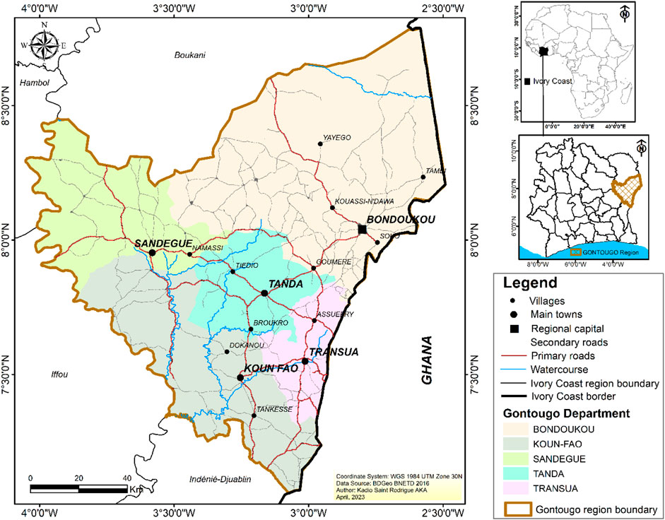
FIGURE 1. Geographic situation of the Gontougo Region.
The soils of the region are generally ferritic, more or less desaturated, deep sandy-clay, and very suitable for cash crops (cashew, cocoa, coffee, and rubber) and food crops (e.g., yams, cassava, rice, maize, and tomatoes) (République de Côte d’Ivoire, 2019). According to the climatic division of Côte d'Ivoire, there are three climatic zones (Kouame, 2021; Kouame et al., 2020): northern, central, and southern zones. The central zone, of which the study area is a part, presents a bimodal seasonal cycle with less pronounced rainfall maximums in June and September. It has four seasons: a long rainy season with frequent rainfall and numerous thunderstorms from April to July, a small dry season in which the sky can remain overcast from August to September, a short rainy season with some small rainfall from September to November, and a long dry season from December to March.
The present study focused on satellite images and field training reference data collected between November and December 2022 in the Gontougo Region to examine LULC change and assess the correlation between NDVI, LULC, and LST. Satellite images include Landsat-8 Oli/Tirs and Sentinel-2 Msi.
The Landsat data used are from the United States Geological Surveys (USGS) and consist of Landsat 8 Collection 2 Tier 1 top of atmosphere (TOA) Reflectance. This dataset’s availability at the time of use is from March 2013 to April 2023. We used them through GEE to calculate NDVI and LST. From 2015 to 2022, we used eight images at a rate of one image per year from the same collection (https://developers.google.com/earth-engine/datasets/catalog/LANDSAT_LC08_C02_T1_TOA).
The Sentinel-2 data used are from Copernicus and consist of Harmonized Sentinel-2, MultiSpectral Instrument (MSI), Level-1C. This dataset’s availability at the time of use is from 23 June 2015 to April 2023 (Table 2). We used them through GEE to perform classification and compute the LULC and its changes (change detection). We used two of these images, one in 2015 and the other in 2022 (https://developers.google.com/earth-engine/datasets/catalog/COPERNICUS_S2_HARMONIZED).
GEE is a geospatial cloud platform for data analysis and geo-information application processing. This platform provides free access to huge volumes of satellite data for computing and offers support tools to monitor and analyze environmental features on a large scale. Such facilities have been widely used in numerous studies on land management and planning (Amani et al., 2020; Tamiminia et al., 2020; Ghosh et al., 2022; Pérez-Cutillas et al., 2023). Several programming languages are used for data processing on GEE, including JavaScript coding. Therefore, using the GEE-integrated code editor, we computed and ran our data with the JS application programming interface (API).
According to America’s space agency [Nasa Earth Observation (https://earthobservatory.nasa.gov/)], LST is how hot the “surface” of the Earth would feel to a touch in a particular location, and NDVI is used to quantify vegetation greenness and density and is useful in understanding plant health. Calculations of NDVI for a given pixel always result in a number that ranges from minus one (−1) to plus one (+1); however, no green leaves give a value close to zero. A zero means no vegetation, and close to +1 (0.8–0.9) indicates the highest possible density of green leaves.
The thermal bands of Landsat images from OLI/TIRS were used to calculate the LST. Single-channel Landsat 8 images were utilized to derive LST (band 10 for each year). For determining LST, it employs the brightness temperature of one band of thermal infrared (TIR), as well as the mean and differential in land surface emissivity (Benmecheta, 2016; Schmugge et al., 2020; Abulibdeh, 2021; Moisa et al., 2022c).
The first step in calculating LST from the metadata of Landsat image files was to convert the digital number to radiance for Landsat OLI/TIRS before calculating brightness temperature (Schmugge et al., 2020; Moisa et al., 2022a; Moisa et al., 2022b). The Landsat 8 OLI digital numbers (DNs) of band 10 were first converted to spectral radiance:
where Lλ is the top of atmosphere (TOA) spectral radiance in watts/(meter squared ster µm), ML is a band-specific multiplicative rescaling factor from the metadata (RADIANCE_MULT_BAND_x, where x is the band number), AL is the band-specific additive rescaling factor from the metadata (RADIANCE_ADD_BAND_x, where x is the band number), QCal corresponds to band 10 and has quantized and calibrated standard product pixel values (DN); TOA = 0.0003342 * “Band 10” + 0.1.
Based on land surface emissivity, atmospheric trans-emissivity, brightness temperature, and average atmospheric temperature, the mono-window algorithm is used to determine LST (Benmecheta, 2016; Huang et al., 2020; Moisa et al., 2022c):
where BT is an effective at-sensor brightness temperature (K); K1 indicates band-specific thermal conversion constant from the metadata (K1_CONSTANT_BAND_x, where x is the thermal band number) (W/(m2 sr μm)); K2 is band-specific thermal conversion constant from the metadata (K2_CONSTANT_BAND_x, where x is the thermal band number) (K); Lλ is spectral radiance at the sensor’s aperture (W/(m2 sr μm)), Lλ = TOA.
Therefore, to obtain the results in Celsius, the radiant temperature is adjusted by adding absolute zero (approx. −273.15°C).
BT = (1321.0789/Ln ((774.8853/“%TOA%”) + 1))—273.15.
The NDVI formula is written according to Aka et al. (2022), Dibi N’da et al. (2008), and Sharifi (2018) as follows:
where NIR means near-infrared, corresponding to band B5, and R indicates red, corresponding to band B4.
Not4e that the calculation of the NDVI is important because, subsequently, the proportion of vegetation (PV), which is highly related to the NDVI, and emissivity (ε), which is related to the PV, must be calculated.
PV is the vegetation proportion acquired according to the formula of Carlson and Riziley (1997) as follows:
According to Sobrino et al. (2004) and Gogoi et al. (2019), the land surface emissivity was computed as follows:
The value of 0.986 corresponds to the correction value of the equation.
Finally, the LST equation is applied to obtain the surface temperature maps. The calculated radiant surface temperatures were corrected for emissivity as follows (Moisa et al., 2022):
LST = [BT/((1 + (0.00115 * BT/1.4388) * Ln (&epsi)—273.5)]where LST means land surface temperature (in Kelvin); BT indicates brightness surface temperature (in Kelvin); λ is the wavelength of emitted radiance (10.8 μm); ρ means h × c/σ (1.438 × 10⁻² mK), in which h is Planck’s constant (6.26 × 10⁻³⁴ J s), c is the velocity of light (2.998 × 10⁸ m/s), and σ is Stefan Boltzmann’s constant (1.38 × 10⁻²³ J/K); and ε is land surface emissivity.
A 3-week field mission in the Gontougo Region collected 390 samples of training points distributed over each land use unit. These data were used to classify the two (2) Sentinel-2 images by training the RFA on 60% of these data and 40% for testing. The spatial distribution of the data collected on the ground on the 2022 Sentinel-2 image is as follows (Figure 2).
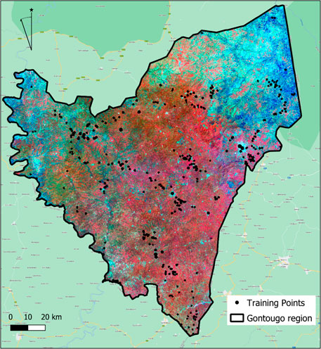
FIGURE 2. Distribution of point samples collected for classification.
This step led us to define and adopt the legend according to the major LULC units found in the field. Thus, six classes were retained, as described in Table 1.
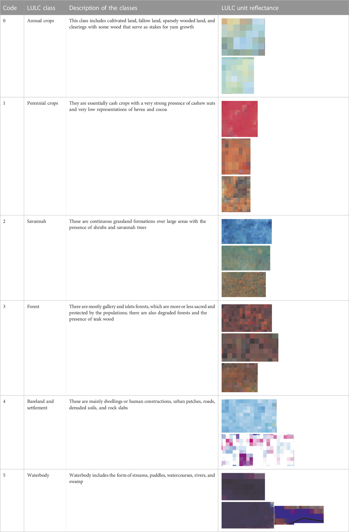
TABLE 1. Description of land occupation units according to the field.
We loaded the Sentinel-2 image collection and applied the filters to them to select the images of the study area. Subsequently, we applied the mask and the mosaic and made the clip. The filters are filter date, filter bounds, cloud cover, cloud pixel, and select bands.
Before moving on to the classification, it is important to calculate the biophysical indices in order to highlight the spectral characteristics of the LULC units according to their reflectance (Aka et al., 2022; Dibi N’da et al., 2008; Kadio et al., 2022). Therefore, we automatically calculated four indices: Soil Index (SI), NDVI, Enhanced Vegetation Index (EVI), and Soil Adjusted Vegetation Index (SAVI) (Morawitz et al., 2006; Zheng et al., 2014; Barriguinha et al., 2022). Then, we combined them with the clipped images of the study area to create new channels; stacked them together to enhance the reflectance of the units present; and achieved less confusion, better classification, and good accuracy. They were calculated according to the following scripts:
//Soil index (SI)
var SI = image. expression (' ((65536-Green)*(65536-Blue)*(65536-Red))’, { 'Red':image.select (['B4']), 'Green':image.select(['B3']), 'Blue':image.select(['B2']) }
//Normalized Difference Vegetation Index (NDVI)
var NDVI = image.normalizedDifference(['B8′, 'B4']).rename('NDVI’);
//Enhanced Vegetation Index (EVI)
var EVI = S2.expression('2.5 * ((NIR -RED)/(NIR +6 * RED -7.5 * BLUE +1))’,
//Soil Adjusted Vegetation Index (SAVI)
var SAVI = S2. expression ('float (((NIR - RED)/(NIR + RED + L))* (1 + L))',{ 'L': 0.5}
//Compilation of Sentinel-2 bands and calculated indices
var compositeS2SS = S2. addBands (si). addBands (ndvi). addBands (evi). addBands (savi).
Map.addLayer (compositeS2, viparams, "compositeSS");
Random Forest (RF) is an ML algorithm used for satellite image classification and geo-information processing. It is a powerful algorithm for feature selection as it ranks the importance of each input variable based on how much it contributes to the overall accuracy (OA) of the classification (Teluguntla et al., 2018; Suryono et al., 2021; Yan et al., 2022; Ashane et al., 2023; Zhao et al., 2023).
We defined the code of each class and gave it the name of the LULC units. Subsequently, the points of the LULC samples collected were distributed: 60% were used for training and 40% for testing:
//Classification functions
Class code = [0, 1, 2, 3, 4, 5]
Class code rename = OCS = ["Annual crops”, "Perennial crops”, "Savannah”, "Forest”, "Bareland and Settlement”, "Waterbody"]; //Distribution of training and testing points
//Training 60%
var training_22 = RedRegions_S2SS.filter (ee.Filter.lt ('random’, 0.6));
//Testing 40%
var testing_22 = RedRegions_S2SS.filter (ee.Filter.gte ('random’, 0.4));
The RFA (smileRandomForest) was applied to the set of stacker images for 2022 and 2015, and then, the algorithm was executed:
var Classification = function (training, label, bands, image, testing) {}
var trainedRF = ee. Classifier.smileRandomForest (100). train ({ features: training, classProperty: label, inputProperties: bands, }); var classifiedRF = S2. select (bands). classify (trainedRF)
The analysis of the changes that occurred over the entire study period was conducted using the two Sentinel-2 images. It produced a change detection matrix from the comparison between the maps of the two dates. Therefore, once the two LULC years have been obtained, we identified the difference between the two dates (Kafi et al., 2014; Gou et al., 2022; Aniah et al., 2023) and then obtained the change according to the following script:
//Define a function to compute change detection using the LULC maps
function compute_change (lulc1, lulc2) {
var change = lulc2. subtract (lulc1);
//Mask out areas where the LULC did not change
var mask = change. neq (0);
change = change. updateMask (mask);
//Return the change map
return change; }
//Compute change maps for 2015 and 2022
var change_2015_2022 = compute_change (lulc_2015, lulc_2022);
Notably, the LULC results obtained from GEE have been geo-processed using ArcGIS software to give the best possible representation of the different land uses and land cover that the Gontougo Region reflects, which is one of the limitations to this study.
The classification details and accuracy are generated using the RFA functions. The function that displays them on GEE is "print” (Ghayour et al., 2021; Aniah et al., 2023). There are error matrix, kappa, OA, producer accuracy, user accuracy, and the classification score for each LULC class:
print (′Training Results RF′,TrainingResults_RF);
print (′RF Matrice Confusion: ′, cmRF);
print (′RF Produceers accuracy: ′, paRF);
print (′RF Users/Cons accuracy: ′, caRF);
print (′Validation Results RF′,results_RF);
The overall change rate (Tg) is used to estimate the overall progress (the proportion of gain or loss) of the areas of LULC units (Dahan et al., 2021; Aka et al., 2022). It is obtained from the following mathematical formula:
where Tg is the overall rate of change (%); S1 represents the area of the class on date t₁ (initial date); S2 is the area of the class on the date t₂ (final date), and t₂ ˃ t₁.
We used the Pearson correlation coefficient, also known as the Pearson R statistical test, to measure the strength between the different variables and their relationships (Eq. (8)). Here, we measured a statistical test between two variables (NDVI and LST). Therefore, according to previous studies (Zheng et al., 2014; Peng et al., 2020), the calculation of the correlation coefficient value enables comprehension of the strength of the relationship between the two variables. Pearson correlation coefficient can range from +1 to −1, where +1 indicates the perfect positive relationship between the variables considered, −1 indicates the perfect negative relationship between the variables considered, and 0 indicates no relationship between the variables considered (Zheng et al., 2014; Njoku and Tenenbaum, 2022):
where rxy is Pearson r correlation coefficient between x and y, n represents the number of observations, xi means the value of x (for ith observation), and yi indicates the value of y (for ith observation).
Through qualitative and quantitative comparison of the change, the LULC types were compared with the LST values over the classification years based on their respective changes (Moisa et al., 2022a).
Over the study period, between 2015 and 2022, the NDVI of the Gontougo Region was determined according to the NIR and Red multispectral bands of the Landsat images. We noticed that the year 2021 presented the highest NDVI mean value with 0.246 and the year 2016 presented the lowest with 0.205 (Table 2). Each NDVI value per year of study was statistically presented in a histogram. These histograms show the distribution of vegetation cover according to the channel in which the NDVI value is high, medium, or low (Figure 3). The distribution of NDVI revolves around the mean values where the highest peaks are observed.
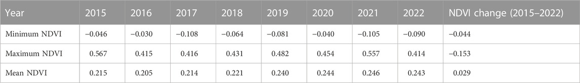
TABLE 2. NDVI minimum, maximum, and mean values per year.
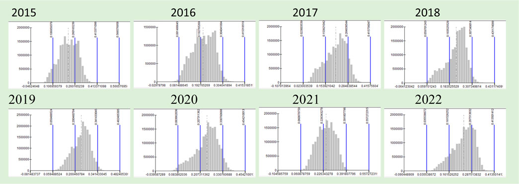
FIGURE 3. NDVI histograms per year.
Qualitatively, the results show that the northeast, northwest, and west parts are much more devoid of vegetation than the other parts of the study area. The central and southern areas have some greenery. Overall, the values vary from −0.108 to 0.566 (Figure 4). The mean values of each NDVI were extracted to appreciate the trend of the vegetation (Figure 5), and the years 2019–2022 showed higher average vegetation than the years 2015–2018, in which the trend was lower.

FIGURE 4. NDVI maps from 2015 to 2022.
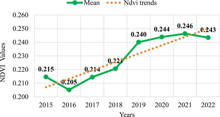
FIGURE 5. Gontougo NDVI mean over time.
The LST is used to monitor the temperature and surface processing of land features. In the present study, LST is calculated using thermal bands from Landsat images from 2015 to 2022. Table 5 reveals that the maximum temperature peaked at 50.11°C in 2021, whereas the minimum temperature was recorded at 9.21°C in 2019. Overall, LSTs are around 31°C when considering mean values. Similarly, at the mean level, there has been a temperature decrease of 0.19°C from 2015 to 2022 (Table 3).
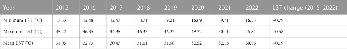
TABLE 3. LST minimum, maximum, and mean values per year.
To better appreciate these values, we generated histograms for each year of LST. These histograms show the distribution of LST values. The horizontal axis shows the minimum values at the beginning and middle, and the mean and maximum values at the end. On the vertical axis, we can see the evolution, especially the concentration of the LST values from the diagonal line (Figure 6). For all years, the distribution of LST is more or less concentrated on the mean in which the highest peaks are observed.
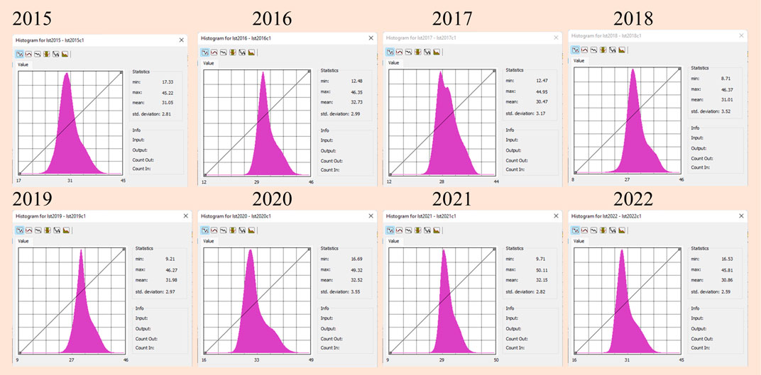
FIGURE 6. LST histograms per year.
The findings of the study revealed that the northeastern and some western parts of the study area had high LST except in the year 2019, when the western part was not high, whereas the southern and center-eastern parts had low LST (Figure 7).
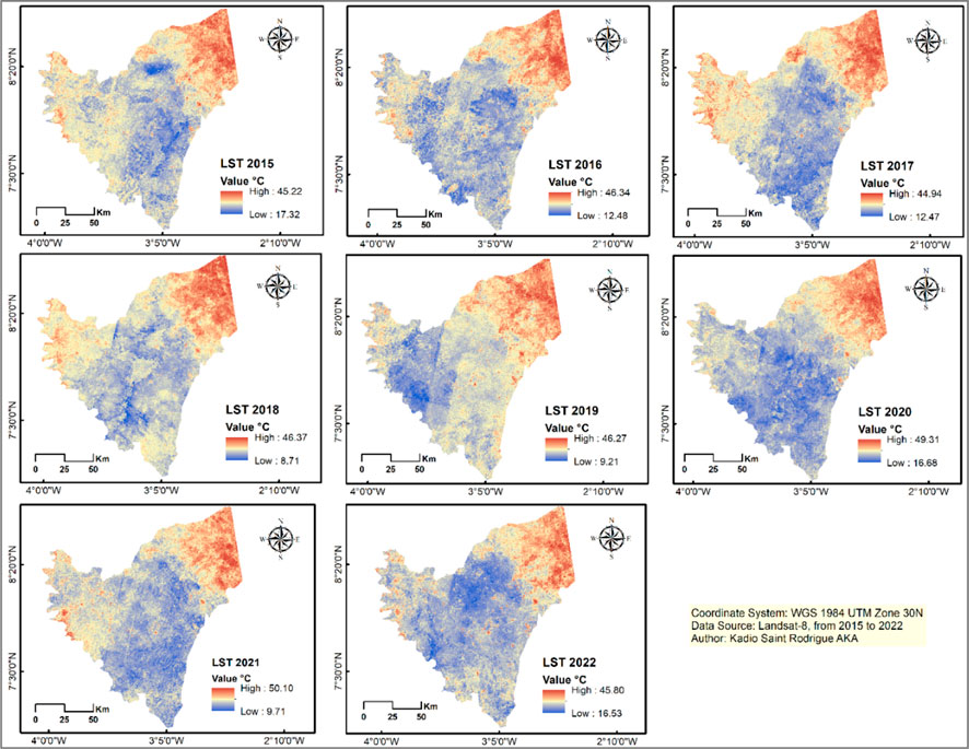
FIGURE 7. LST maps from 2015 to 2022.
Based on the mean values, we represented the trend of the LST. The year 2017 recorded the lowest temperature at 30.47°C, and the year 2016 had the highest temperature at 32.73°C. The overall trend shows a constant and slight evolution along the LST trend line (Figure 8).
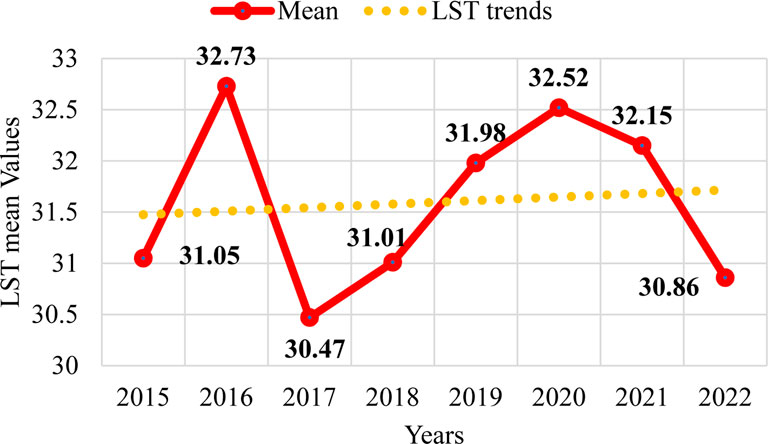
FIGURE 8. Gontougo LST mean over time.
All the results in this section were obtained from the classification of Sentinel-2 images using GEE. Therefore, we used the following abbreviations: UA, user accuracy; PA, producer accuracy; OA, overall accuracy; Acrops, annual crops; Pcrops, perennial crops; Sav, savannah; Forest, forest; BarSet, bareland and settlement; Wb, waterbody.
Accuracy assessment is a process that evaluates the accuracy of a LULC classification map (the classified data) by comparing it to reference data (Olofsson et al., 2013; Aniah et al., 2023). The field sample of the LULC units serves as our reference data. Accuracy assessment provides a quantitative measure of the classification’s OA and identifies the LULC classes where errors are prevalent. Thus, we determined the following precision statistics for each classification: F1 score, PA, and UA (Table 4). The F1 score considers precision (PA and UA) and recall so that the two reach the highest values at the same time and balance (Zhang et al., 2023). In our situation, the BarSet class has the greatest score for the year 2015 (0.98), whereas Acrops has the lowest (0.70). For the year 2022, the highest score is the Wb class (1.00) and the lowest is Acrops (0.83). The percentage of pixels in each correctly classified class to all the pixels in that class in the reference data determines the producer accuracy in Table 6. It evaluates how accurately a classification can identify a given class. Subsequently, user accuracy is the proportion of correctly classified pixels in each class to the total number of pixels in that class in the classification map. It measures the accuracy of classification in correctly assigning pixels to a particular class (Jensen J. R., 1986; Congalton, 1991; Olofsson et al., 2013; Rwanga and Ndambuki, 2017; Aniah et al., 2023; Zhang et al., 2023). In our situation, we had low values of PA and UA in 2015 of 0.73 and 0.67, respectively, which belonged to classes Acrops and Sav. In addition, high values of 0.96 and 1.00 belong to classes Pcrops and Wb, respectively. Following the year 2022, the trend was better, and we had low values of PA and UA of 0.80 and 0.81, belonging, respectively, to the Savannah and Acrops classes, and a high value of 1.00 of each side belonging to classes Wb and BarSet for PA and Wb for UA. Figure 9 graphically shows the precision with all the different values on the vertical axis.
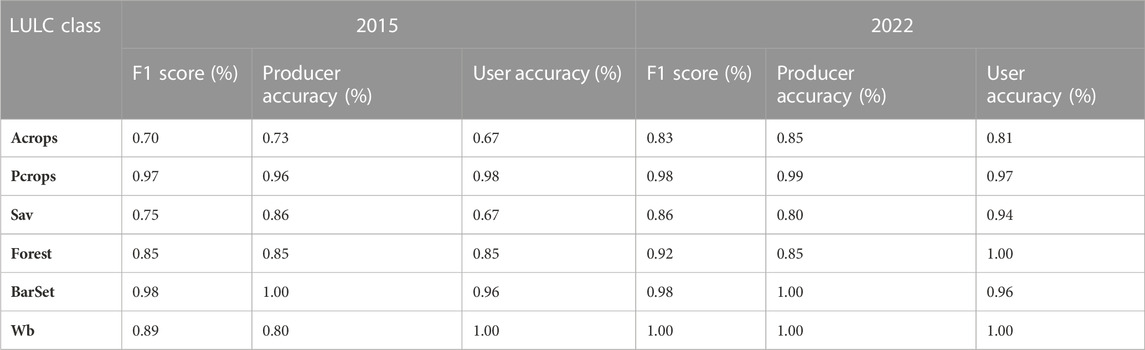
TABLE 4. Sample training data classification precision by LULC class.
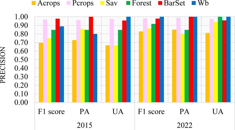
FIGURE 9. Samples precision of the LULC mapping for 2 years.
The overall cartographic accuracy and kappa coefficient of the classification process on the two Sentinel-2 images are presented in Tables 5, 6 (error matrices). For each year’s classification, we calculated the OA and kappa to evaluate the accuracy of the classification results. OA is the proportion of correctly classified pixels to the total number of pixels in the image. It provides a measure of the classification’s OA. The kappa coefficient is a measure of agreement between the classification map and the reference data that considers the possibility of chance agreement. It ranges from −1 to 1, with one indicating perfect agreement and 0 indicating no agreement beyond chance (Congalton, 1991; Banko, 1998; Rwanga and Ndambuki, 2017; Aka et al., 2022; Zhang et al., 2023). In the 2015 LULC classification, the OA was 0.94%, and the kappa was 0.87. However, in the year 2022, the OA was 0.96% and the kappa 0.92. The diagonal values in the gray font represent the well-classified pixels between UA and PA, and the other values represent the commission and omission errors. Both errors occur during LULC mapping. Indeed, an error of omission refers to when a feature that should have been mapped was missed, whereas an error of commission occurs when a feature is mapped that should not have been included in the LULC classification (Congalton, 1991; Banko, 1998; Akomolafe and Rosazlina, 2022).
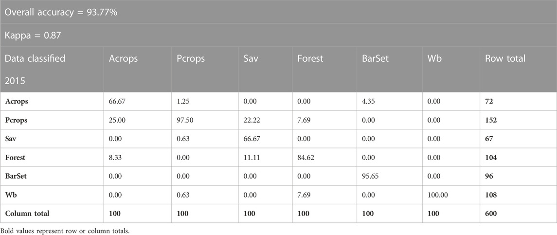
TABLE 5. LULC error matrix, 2015.
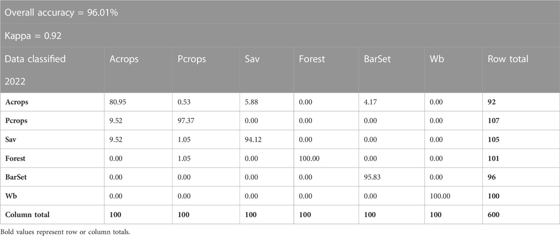
TABLE 6. LULC error matrix, 2022.
The LULC mapping of the study area led to two maps, each showing the following six classes: annual crops, bareland and settlement, forest, perennial crops, savannah, and waterbody (Figure 10). At first glance, we can see the regression of forest and annual crop classes between the two dates. The savannah class is more present in the northeast and the extreme west, and little represented in the central region where the forest is dominant. The waterbody class is very thin and almost invisible. However, it can be observed on the western side in the year 2015, where a river flows, of which the study area is the limit. Generally, water in the research region is mostly in the form of puddles, ponds, and wetlands, which dries up during the dry season leaving bare soil. The bareland and settlement class is disseminated and more present in the northwest on both images and accentuated in 2022. Finally, the perennial crop class, the most obvious and visible in both images, occupies the largest area (63% in 2015% and 67% in 2022) of all LULC classes (Table 7).
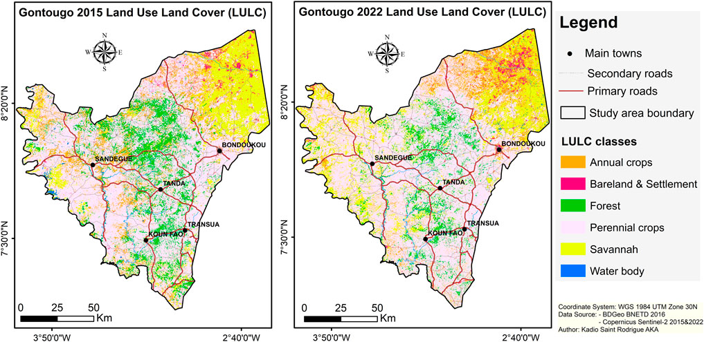
FIGURE 10. Gontougo LULC map of 2015 and 2022.
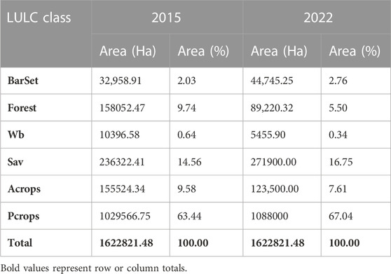
TABLE 7. LULC area in hectares and percentage.
The overall rate of LULC changes made it possible to estimate the overall increase in the gain and loss proportion of LULC areas (Aka et al., 2022). Analysis of the rate of change shows that BarSet, Sav, and Pcrops have positive values and indicate a “gain or progression in the area.” Forest, Wb, and Acrops have negative values, thus indicating a “loss or regression in the area” (Figure 11). The critical loss is Wb (−47.52%), and the most gain is for the BarSet (35.76%) class.
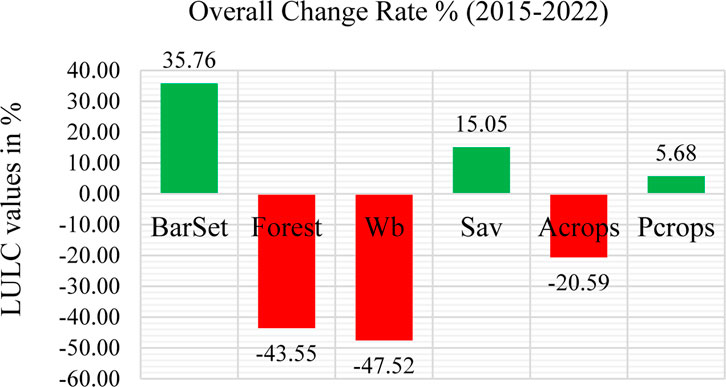
FIGURE 11. Overall rate of LULC changes in the study area between 2015 and 2022.
The assessment of the overall LULC change rate led us to set up and calculate the LULC change matrix, also called the transition matrix. The LULC change matrix is used to quantify changes in the distribution of LULC types over time. We used it to monitor and analyze changes between the 2015 and 2022 LULC maps. The matrix rows represent the LULC types in the earlier period, whereas the columns represent the LULC types in the later time. The matrix cells show the areas converted from one LULC type to another. However, the diagonal values in gray color represent the percentages of LULC classes that remained stable. Only 13.40% of the Acrops areas have remained stable, and 65.14% have been converted into Pcrops, which is alarming (Table 8). These statistics can be seen in detail with the overall area in hectares, the percentage of each LULC type, and the changes it has experienced from 2015 to 2022 in Table 9. As shown in the area column (in percentage), the values in gray color stand for LULC classes that remained stable, and the other values have undergone mutations by moving from one class to another.
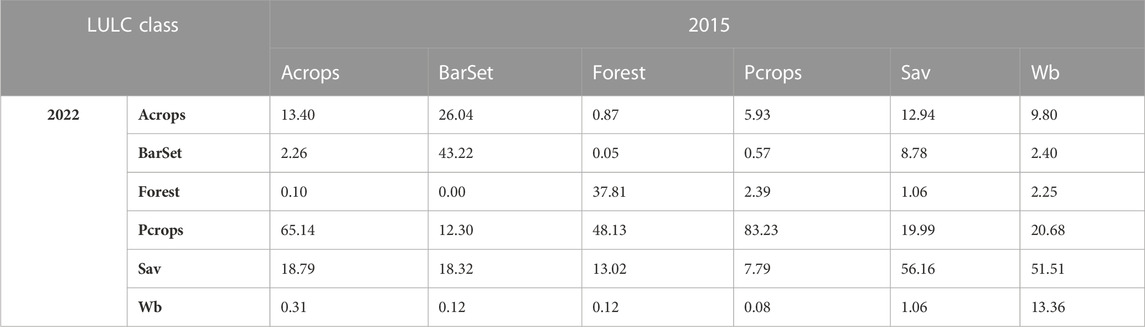
TABLE 8. LULC change matrix in percentage between 2015 and 2022.
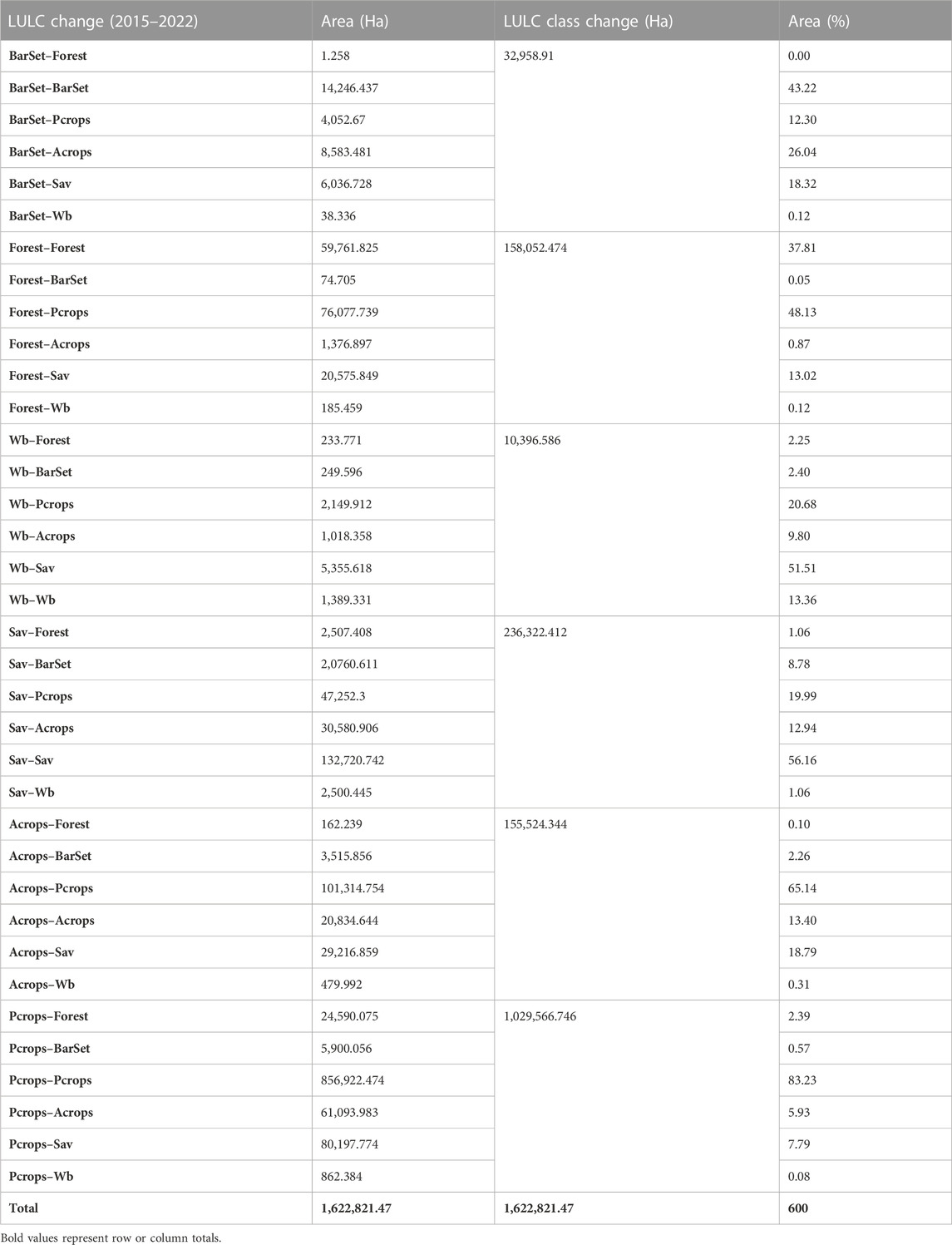
TABLE 9. LULC change matrix details between 2015 and 2022.
The relationship between LST and NDVI was examined using Pearson correlation analysis. Pearson correlation is a measure of the linear relationship between two variables. It ranges from −1 to 1, where −1 indicates a perfectly negative correlation, 0 indicates no correlation, and one indicates a perfectly positive correlation. It is used in statistics to examine the strength and direction of the relationship between two variables (Zheng et al., 2014; Abulibdeh, 2021). We performed statistical analysis by comparing the LST and NDVI values after reclassification in which both variables had the same number of classes. We had eight images on each side; therefore, eight matches were made per pair (LST and NDVI together). The LST values ranged from maximum (50.11°C) to minimum (9.21°C) temperatures, whereas the NDVI values ranged from 0.567 to −0.108, from maximum to minimum. The results show that LST and NDVI have a strong negative correlation each year (Table 10). Following Table 12, which shows the type of correlation between NDVI and LST, we investigated the plots generated by these tables, which show how the regression line declines at each correlation (Figure 12). This indicates a negative correlation between NDVI and LST. Hence, the Pearson correlation coefficient (r) recorded at each correlation indicates negative values from 2015 to 2022. These values are −0.992, −0.982, −0.975, −0.977, −0.966, −0.994, −0.990, and −0.978, respectively, from 2015 to 2022.
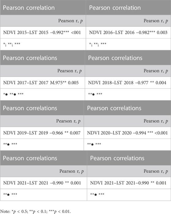
TABLE 10. Pearson’s correlation coefficient (r) between NDVI and LST.

FIGURE 12. Pearson correlation (scatter plots) between NDVI and LST.
The distributions of spatial LST values for the different LULC classes were reclassified and mapped for the two LULC years, 2015 and 2022, to depict temperature differences on the maps and show the LULC areas that are more or less heated (Figure 13). These LST values reclassify maps to show that the hottest areas are the savannah and the bareland and settlement. The results are similar for the low-temperature areas, which are more or less forest areas. In addition, there is a significant spread of LULC classes and temperatures that vary immensely over the whole area on both maps. Furthermore, the surface temperatures varied between 17.33°C and 45.22°C in 2015 and 16.53°C and 45.81°C in 2022. These values can be observed on the map through the legend.
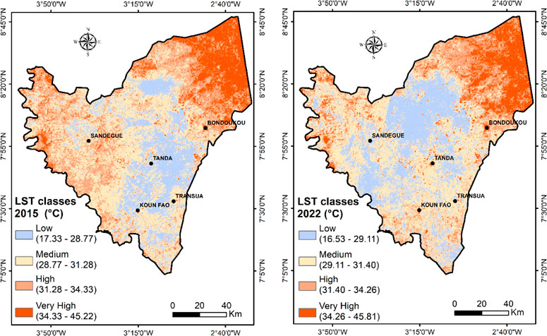
FIGURE 13. LST reclassification.
Subsequently, the mean LST values were matched to the LULC classes. In 2015, the bareland and settlement class recorded the highest surface temperature (35.18°C), followed by the Savannah class (34.60°C). The forest class recorded the lowest temperature (28.69°C) (Table 11). In 2022, still with the mean LST values, the correlation showed again that the bareland and settlement class recorded the highest LST at 35.41°C, and the lowest LST was recorded for the forest class (28.46°C). The differences in mean temperature are a decrease in LST of 0.23 for the forest class and an increase for the bareland and waterbody classes.
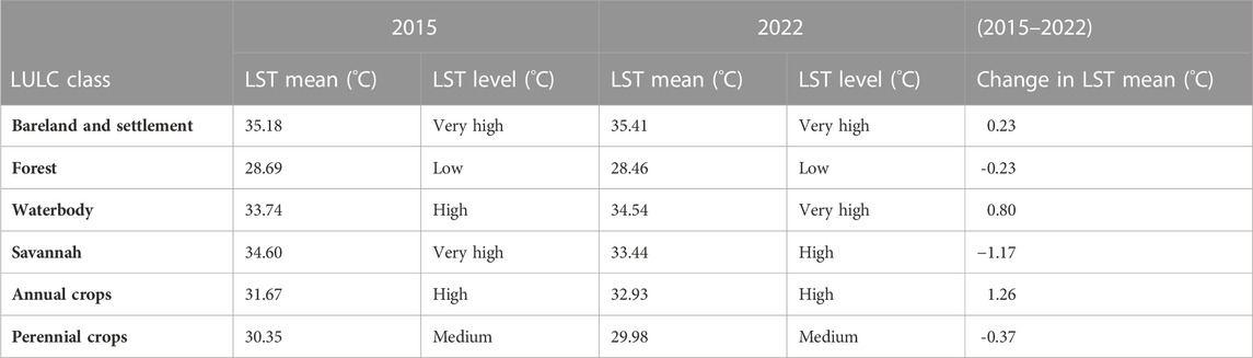
TABLE 11. Correlation between LULC and LST.
The spatiotemporal analysis of the Gontougo LULC change made it possible to categorize six LULC classes each year: annual crops, perennial crops, savannah, forest, bareland and settlement, and waterbody. The OA obtained is 93.77% with a kappa coefficient of 0.87 for the year 2015 map and 96.01% OA and 0.92 kappa coefficient for the year 2022 map. These results are close to those obtained by Kadio et al. (2022), who mapped the Sentinel-2 image and compared it with Landsat-8 Oli in the Azagny site Ramsar in Côte d’Ivoire. The OA was 90.63%, and the kappa was 0.94. In addition, Zhang et al. (2023) used GEE and RF with three Sentinel-2 images in the crop mapping type for agronomic purposes to quantify cultivated areas and determine yields in China. They obtained 95.72%, 97.21%, and 98.13%, respectively, as OA and 0.94, 0.96, and 0.98 as kappa for the years 2017, 2018, and 2020. This latter study is somewhat similar to ours in the sense that it discusses the use of ML and RFA and highlights all the cartographic precision obtained in this study. In remote sensing, a classification is deemed acceptable when the kappa coefficient value is greater than 75% (Jensen J. R., 1986; Congalton, 1991; Zhang et al., 2023). It confirms that the results of this analysis are statistically acceptable. Currently, RFA is widely used in satellite image classification because it gives better results (Teluguntla et al., 2018; Phalke et al., 2020; Yan et al., 2022; Zhao et al., 2023). We are increasingly turning to ML technology, such as GEE, to implement LULC change. These authors also performed the same in their LULC study using Landsat collection images (Teluguntla et al., 2018; Phalke et al., 2020; Suryono et al., 2021; Yan et al., 2022; Ashane et al., 2023; Zhao et al., 2023). The particularity of our study here is to use Sentinel-2, which is one of the studies that has so far mapped the LULC change in the entire Gontougo Region and assessed the LST using ML technology (GEE) and RFA. However, it should be noted that Sentinel-2A was launched in June 2015, and the first images were available on 23 June 2015. These early images of the Sentinel-2 mission over our study area showed quite a bit of artifact and constituted bits of images with continuous haze. The mosaicking and speckle cleaning gave us a homogeneous image from which the 2015 classification was made. This justified the low precision obtained compared to 2022, when the filter interval search was conducted over a full year.
The other striking aspect of our research is the drastic loss of forests and the dramatic decrease in annual crop areas. Indeed, from 2015 to 2022, forests lost 62.19% of their area, and annual crops lost 86.6% of their area. These various losses benefit perennial crops by up to 48.13% for the forest and 65.14% for annual crops. Indeed, according to a study conducted in the region on the re-profiling of roads by the State of Cote d'Ivoire, and according to the latest census of the population and habitat, the Gontougo Region’s potential economy is based primarily on agriculture, and the reputation of this region is based on the famous variety of yam called “Kponan” (République de Côte d’Ivoire, 2019; RGPH-CI, 2021). The current situation shows a landscape strongly dominated by perennial crops, with cashew nuts in the lead. The region is one of the largest cashew producers in Côte d’Ivoire, with 65,018 tons in 2022, according to the Cashew Cotton Council (CCA). In detail, at the level of each Gontougo department, it is 49,735 t in Bondoukou, 3,315 t in Koun Fao, 7,725 t in Sandégué, 4,094 t in Tanda, and 194 t in Transua. These statistics are given by the Agence Ivoirienne de Presse (AIP) in an article published on 3 February 2023 at 8:01 GMT entitled «Côte d'Ivoire—AIP/Noix de cajou: L'Indénié-djuablin et le Gontougo ont réalisé une production annuelle de 68,697 tonnes en 2022» and edited by Memel Franck Niagnely1. This necessitates the availability of a large production area and explains why the vegetation cover and yearly crop area have been drastically reduced. As for the yam crop, in most cases, it is used to prepare or lay out the soil for the next cashew season. According to the yam farmers themselves, they transplant small cashew seedlings into their producing yam fields. After the yam harvest, the cashew field takes over completely, and new annual crop areas are sought for the following year. This is one of the factors contributing to the annual decline in the area planted for annual crops. The fact that annual crops are not grown in isolation and that it is important to leave trees in the fields of annual crops, particularly yam, to encourage the growth of yam buds, also serves to justify the low precision of mapping technically and discrimination of the annual crops class1.
Land surface heating is the cumulative effect of LULC change and global atmospheric warming (Moisa et al., 2022b; Moisa et al., 2022c). The decline in vegetation cover driven by agricultural expansion in the study area substantially increases the LST. Indeed, the results show that the lowest observed temperatures are in areas where forests are present. Respectively, the LULC forest areas of 2015 and 2022 recorded the lowest mean LST of 28.69°C and 28.46°C. This translates into a slight decrease in temperature over the year. This trend is verified within NDVI calculations. According to some authors (Carlson and Riziley, 1997; Davi et al., 2006; Morawitz et al., 2006; Du et al., 2017; Wu et al., 2019; Syawalina et al., 2022), healthy vegetation absorbs most of the visible light that hits it and reflects a large portion of the near-infrared light. Unhealthy or sparse vegetation reflects more visible and less near-infrared light (Davi et al., 2006; Dibi N’da et al., 2008; Khan et al., 2010; Phan et al., 2021). Therefore, NDVI has a huge influence on LST calculation and the surface temperature content. Therefore, we used it to correlate with the LST. Similar to the LST, NDVI was reclassified into four classes and was well-corrected with the LST (Table 12). This NDVI classification corresponds to the vegetation standards from sub-Saharan humid tropical countries because the definition of the forest depends on the forestry code of each country (Dibi N’da et al., 2008; RCI-Code Forestier, 2019b; RCI-Code Forestier, 2019a). Accordingly, the negative NDVI values corresponding to the “non-vegetation land” description recorded the highest temperatures. This can also be perceived with the Pearson correlation coefficient (r) for each year (Figure 12) and confirms that the absence of vegetation induces a high surface temperature compared to the vegetated land, which records a low temperature (Zheng et al., 2014). However, the negative Pearson correlation coefficient values found in the relationship between the LST and NDVI indicate that the presence of green areas mitigates the surface temperature effect because the vegetation is wet and contains water almost throughout most months of the year through the leaves compared to other types of LULC. Therefore, it moistens the surface and absorbs more and reflects less solar radiation (Davi et al., 2006; Morawitz et al., 2006).
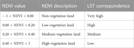
TABLE 12. NDVI classification in correlation with LST.
In contrast, water surfaces have often recorded high temperatures (33.74°C in 2015 and 34.54°C in 2022 for the mean temperature). In fact, the waterbody class is not a large river or big stream. It comprises puddles, backwaters, small lakes, ponds, and swamps. As noticed, it is the class with the smallest extent and represents less than 1% of the total area of the classes in 2015 and exactly 0.34% in 2022. This means that water dries up, especially in the dry season, and becomes bareland. As a result, the temperatures will be very high, like in the bareland and savannah areas. Indeed, our study has shown that the hottest surfaces with the highest temperatures are the bareland/settlement and savannah. The mean temperatures of these LULC classes are 35.18°C and 35.41°C for bareland and settlement, respectively, in 2015 and 2022 and 34.60°C and 33.44°C for savannah, respectively, in 2015 and 2022. The bareland and settlements are devoid of vegetation, and the savannah is dominated by grasses and shrubs, which cannot strongly absorb sun rays. Therefore, reflections are strong, which justifies the high temperatures recorded at these LULC classes. A recent study (Moisa et al., 2022a; Moisa et al., 2022b; Moisa et al., 2022c) on the wettest parts of Ethiopia, covered in the present study, confirmed that the increasing trend of temperature is driven by weak NDVI values and LULC conversion. One of their outputs concerns the great variation between daytime and nighttime temperatures, which can influence the LST. As highlighted by the same authors, the LST increases during the daytime more than at night. Akomolafe and Rosazlina. (2022) found a moderate negative relationship between NDVI and LST in Penang Island, Peninsular Malaysia. This shows that higher LSTs correspond to lower vegetation cover and vice versa, as our results also show. Through the urban heat island characteristics and mitigation strategy analysis of eight arid and semi-arid gulf region cities, Abulibdeh (2021) stated that vegetation, particularly trees, can prevent direct surface heat as a result of solar radiation by providing shade, cooling the air by generating cool island effects, evapotranspiration and emissivity processes, and reducing the wind speed under the canopies. In the Pearson correlation coefficient analysis, the same author (Abulibdeh, 2021) stated that the LST has a significant relationship with NDVI but in different directions. The relationship between the LST and NDVI is negative, indicating that the presence of green areas mitigates the LST preponderance effect. All these claims by different authors confirm our results and demonstrate once again the importance of LULC changes and their effects on the LST modification.
This study examined LULC change analysis and its effects on LST using ML through GEE in the Gontougo Region. Regarding LULC, we could discriminate six classes: annual crops, perennial crops, savannah, forest, bareland/settlement, and waterbody. From 2015 to 2022, the OA values for each LULC map were 93.77% and 96.01%, respectively. Similarly, the kappa was 0.87 in 2015 and 0.92 in 2022. The prevailing LULC class is perennial crops. It occupies more than 60% of the area of each LULC map. LULC change found that the forest and annual crop classes lost 48.13% and 65.14%, respectively, of their areas for the benefit of perennial crops from 2015 to 2022. The NDVI and LST reclassification correspondences have shown that non-vegetation land corresponds to very high temperature, low vegetation land corresponds to high temperature, medium vegetation land corresponds to medium temperature, and high vegetation land corresponds to low temperature. Similarly, their correlation using Pearson coefficient (r) gave a significant relationship, and negative coefficients were obtained for each correlation. In terms of the LST–LULC correlation, the forest class recorded the lowest temperatures each year. In 2015, the mean temperatures recorded were 28.69 °C and 28.46 °C in 2022. Conversely, the highest temperatures were recorded by the bareland/settlement class. A mean of 35.18°C in 2015 and 35.41°C in 2022 were recorded. Therefore, the existence of vegetation coverage was indispensable for decreasing surface temperature. It was recommended that natural resource managers and environmental experts should create awareness and environmental conservation to minimize LST in the study area. Furthermore, the decline in the annual crop area each year to perennial crops should be aware of all decision-makers and farmers in the region that this will lead to a real food security issue. We must raise the alarm so that the crops that feed us directly are brought to the forefront in our choice of crops to be food self-sufficient. This study has benefits for monitoring and evaluating food security in Côte d'Ivoire, adding to the evidence base of other studies on the use of remote sensing to identify crop types and cropping patterns in other countries. However, it should be noted that one of the limitations to this study is that it was not possible to map the yam crop specifically. This would have enabled us to assess the impact of LSTs on yams directly. This aspect will be addressed in future work using very high spatial-resolution images. The results of this study are a response to the food security challenges related to land use in the area. Based on these study results, we plan to conduct a future socio-economic study in which we will gather yam farmers’ perceptions of climate change, the difficulties they face in yam production, and available solutions. In addition, a soil sampling and analysis study is planned to solve the soil fertility problems faced by people in the Gontougo Region.
The datasets presented in this study can be found in online repositories. The names of the repository/repositories and accession number(s) can be found in the article/supplementary material.
Ethical review and approval was not required for the study on human participants in accordance with the local legislation and institutional requirements. Written informed consent for participation was not required for this study in accordance with the national legislation and institutional requirements. Written informed consent was obtained from the individual(s) for the publication of any potentially identifiable images or data included in this article.
All authors listed have made a substantial, direct, and intellectual contribution to the work and approved it for publication.
The authors thank the West African Science Service Centre on Climate Change and Adapted Land Use (WASCAL) for the scholarship which allowed them to embark on this research. They specially thank the National Office for Technical Studies and Development (BNETD) through the Center for Geographic and Digital Information (CIGN), which greatly contributed to facilitating access to data collection in the field at that time.
AG was employed by 3A Environmental Solutions Ltd. EB was employed by Digital Earth Africa.
The remaining authors declare that the research was conducted in the absence of any commercial or financial relationships that could be construed as a potential conflict of interest.
All claims expressed in this article are solely those of the authors and do not necessarily represent those of their affiliated organizations or those of the publisher, the editors, and the reviewers. Any product that may be evaluated in this article, or claim that may be made by its manufacturer, is not guaranteed or endorsed by the publisher.
1https://www.aip.ci/cote-divoire-aip-noix-de-cajou-lindenie-djuablin-et-le-gontougo-ont-realise-une-production-annuelle-de-68-697-tonnes-en-2022/
Abulibdeh, A. (2021). Analysis of urban heat island characteristics and mitigation strategies for eight arid and semi-arid gulf region cities. Environ. Earth Sci. 80, 259. doi:10.1007/s12665-021-09540-7
Aighewi, B. A., Asiedu, R., Maroya, N., and Balogun, M. (2015). Improved propagation methods to raise the productivity of yam (Dioscorea rotundata Poir). Food Secur. 7 (4), 823–834. doi:10.1007/s12571-015-0481-6
Aka, K. S. R., Dibi, H. N., Koffi, J. N., and Bohoussou, C. N. (2022). Land cover dynamics and assessment of the impacts of agricultural pressures on wetlands based on earth observation data: case of the Azagny ramsar site in southern Côte d’Ivoire. J. Geoscience Environ. Prot. 10 (05), 43–61. doi:10.4236/gep.2022.105004
Akomolafe, G. F., and Rosazlina, R. (2022). Land use and land cover changes influence the land surface temperature and vegetation in Penang Island, Peninsular Malaysia. Sci. Rep. 12, 21250. doi:10.1038/s41598-022-25560-0
Akpoti, K., Groen, T., Dossou-Yovo, E., Kabo-bah, A. T., and Zwart, S. J. (2022). Climate change-induced reduction in agricultural land suitability of West-Africa’s inland valley landscapes. Agric. Syst. 200, 103429. doi:10.1016/j.agsy.2022.103429
Amani, M., Ghorbanian, A., Ahmadi, S. A., Kakooei, M., Moghimi, A., Mirmazloumi, S. M., et al. (2020). Google earth engine cloud computing platform for remote sensing big data applications: a comprehensive review. IEEE J. Sel. Top. Appl. Earth Observations Remote Sens. 13, 5326–5350. doi:10.1109/jstars.2020.3021052
Aniah, P., Bawakyillenuo, S., Codjoe, S. N. A., and Dzanku, F. M. (2023). Land use and land cover change detection and prediction based on CA-Markov chain in the savannah ecological zone of Ghana. Environ. Challenges 10, 100664. doi:10.1016/j.envc.2022.100664
Ashane, M., Fernando, W., and Senanayake, I. P. (2023). Developing a two-decadal time-record of rice field maps using landsat-derived multi-index image collections with a random forest classifier: a google earth engine based approach. Inf. Process. Agric. 23, 1–35. doi:10.1016/j.inpa.2023.02.009
Asselin, O., Leduc, M., Paquin, D., Winger, K., Luca, A., Music, B., et al. (2022). Climate response to severe forestation: a regional climate model intercomparison study. EGUsphere. [Preprint]. doi:10.5194/egusphere-2022-291
Banko, G. (1998). A review of assessing the accuracy of classifications of remotely sensed data and of methods including remote sensing data in forest inventory. Avaliable At: www.iiasa.ac.at.
Barrie, L., and Braathen, G. (2021). Wmo greenhouse gas bulletin: the state of greenhouse gases in the atmosphere based on global observations through 2020. Avaliable At: https://ig3is.wmo.int/.
Barriguinha, A., Jardim, B., de Castro Neto, M., and Gil, A. (2022). Using NDVI, climate data and machine learning to estimate yield in the Douro wine region. Int. J. Appl. Earth Observation Geoinformation 114, 103069. doi:10.1016/j.jag.2022.103069
Benmecheta, A. (2016). Estimation de la température de surface a partir de l’imagerie satellitale; validation sur une zone côtière d’Algérie. Avaliable At: https://tel.archives-ouvertes.fr/tel-01565894.
Carlson, T. N., and Riziley, D. A. (1997). On the relation between NDVI, fractional vegetation cover, and leaf area index. Remote Sens. Environ. 62, 241–252. doi:10.1016/S0034-4257(97)00104-1
Congalton, R. G. (1991). A review of assessing the accuracy of classifications of remotely sensed data. Remote Sens. Environ. 37, 35–46. doi:10.1016/0034-4257(91)90048-B
Dahan, K. S., Dibi N’da, H., and Kaudjhis, C. A. (2021). Dynamique spatio-temporelle des feux de 2001 à 2019 et dégradation du couvert végétal en zone de contact foret-savane, Département de Toumodi, Centre de la Côte d’Ivoire in Afrique SCIENCE. Avaliable At: https://ladsweb.modaps.eosdis.nasa.gov/.
Davi, H., Soudani, K., Deckx, T., Dufrene, E., Le Dantec, V., and François, C. (2006). Estimation of forest leaf area index from SPOT imagery using NDVI distribution over forest stands. Int. J. Remote Sens. 27 (5), 885–902. doi:10.1080/01431160500227896
Dibi N’da, H., Kouakou N’guessan, E., Wajda, M. E., and Affian, K. (2008). Apport de la télédétection au suivi de la déforestation dans le Parc National de la Marahoué (Côte d´Ivoire). Teledetection 8 (1), 17–34.
Diulyale, K., Yaya, T., Kassi, M. F., and Kone, T. (2019b). Structuration de la population agricole de la filière anacarde (Anacardium occidentale(L) Anacardiaceae) et caractérisation des plantations dans les régions du Bounkani et du Gontougo en Côte d’Ivoire. Int. J. Innovation Appl. Stud. 26 (4), 1159–1169.
Diulyale, K., André, S. B., Yaya, T., Tchoa, K., Nakpalo, S., Noémie, R., et al. (2019a). Evaluation de la technique de surgreffage pour le rénouvellement des vieillissants vergers d’anacardier [Anacardium occidentale (L)] dans la région du Gontougo en Côte d’Ivoire. Eur. Sci. J. ESJ 15, 304. doi:10.19044/esj.2019.v15n6p304
Du, Z., Zhang, X., Xu, X., Zhang, H., Wu, Z., and Pang, J. (2017). Quantifying influences of physiographic factors on temperate dryland vegetation, Northwest China. Sci. Rep. 7, 40092. doi:10.1038/srep40092
Félicia, J., Guessan, N., Robert, O., Depo’, N., Cherif, M., Johnson, F., et al. (2017). Inventaire des insectes ravageurs du verger anacardier dans les régions de Bounkani, Gontougo et Indénie-Djablun au Nord-Est en Côted’Ivoire Afrique SCIENCE. Avaliable At: http://www.afriquescience.info.
Ghaderizadeh, S., Abbasi-Moghadam, D., Sharifi, A., Tariq, A., and Qin, S. (2022). Multiscale dual-branch residual spectral-spatial network with attention for hyperspectral image classification. IEEE J. Sel. Top. Appl. Earth Observations Remote Sens. 15, 5455–5467. doi:10.1109/jstars.2022.3188732
Ghayour, L., Neshat, A., Paryani, S., Shahabi, H., Shirzadi, A., Chen, W., et al. (2021). Performance evaluation of sentinel-2 and landsat 8 OLI data for land cover/use classification using a comparison between machine learning algorithms. Remote Sens. 13, 1349. doi:10.3390/rs13071349
Ghosh, S., Kumar, D., and Kumari, R. (2022). Cloud-based large-scale data retrieval, mapping, and analysis for land monitoring applications with Google Earth Engine (GEE). Environ. Challenges 9, 100605. doi:10.1016/j.envc.2022.100605
Gogoi, P. P., Vinoj, V., Swain, D., Roberts, G., Dash, J., and Tripathy, S. (2019). Land use and land cover change effect on surface temperature over Eastern India. Sci. Rep. 9, 8859. doi:10.1038/s41598-019-45213-z
Gou, y., Louis, V., Roberts, J. F., and Rodriguez-Veiga, P. (2022). Near real-time change detection system using sentinel-2 and machine learning_ A test for Mexican and Colombian forests _ enhanced reader. Remote Sens. 14, 707. doi:10.3390/rs14030707
Huang, R., Huang, J. x., Zhang, C., Ma, H. y., Zhuo, W., Chen, Y. y., et al. (2020). Soil temperature estimation at different depths, using remotely-sensed data. J. Integr. Agric. 19 (1), 277–290. doi:10.1016/s2095-3119(19)62657-2
IPCC (2014). Climate change 2014: Impacts, adaptation, and vulnerability. Working group II contribution to the fifth assessment report of the Intergovernmental Panel on Climate Change. Cambridge, UK/New York, USA: Cambridge University Press. Avaliable At: www.ipcc-wg2.gov/AR5.
IPCC (2023). “Technical summary,” in Climate change 2022 – impacts, adaptation and vulnerability (Cambridge, United Kingdom: Cambridge University Press), 37–118. doi:10.1017/9781009325844.002
Jensen, J. R. (1986). Introductory digital image processing. A remote sensing perspective, xv 379. Englewood Cliffs: Prentice-Hall.
Kadio, S. R. A., Hyppolite, N. D. I. B. I., N’dri Koffi, J., and Crystel, B. N. (2022). Étude comparative de Sentinel-2 et Landsat-8 Oli à l’évaluation de l’occupation du sol du site Ramsar d’Azagny, Sud de la Côte d’Ivoire Afrique SCIENCE. Avaliable At: http://www.afriquescience.net.
Kafi, K. M., Shafri, H. Z. M., and Shariff, A. B. M. (2014). An analysis of LULC change detection using remotely sensed data; A Case study of Bauchi City. IOP Conf. Ser. Earth Environ. Sci. 20, 012056. doi:10.1088/1755-1315/20/1/012056
Khan, M. R., de Bie, C. A. J. M., van Keulen, H., Smaling, E. M. A., and Real, R. (2010). Disaggregating and mapping crop statistics using hypertemporal remote sensing. Int. J. Appl. Earth Observation Geoinformation 12 (1), 36–46. doi:10.1016/j.jag.2009.09.010
Kosari, A., Sharifi, A., Ahmadi, A., and Khoshsima, M. (2020). Remote sensing satellite’s attitude control system: rapid performance sizing for passive scan imaging mode. Aircr. Eng. Aerosp. Technol. 92 (7), 1073–1083. doi:10.1108/aeat-02-2020-0030
Kouakou, A. M., Yao, G. F., Dibi, B., Mahyao, A., Lopez-Montes, A., Essis, B. S., et al. (2019). Yam cropping system in Cote d’Ivoire: current practices and constraints. Eur. Sci. J. 15, 278. doi:10.19044/esj.2019.v15n30
Kouame, K. F. (2021). “Analyse comparative des données satellitaire d’estimation des précipitations en Côte d’Ivoire. These de Doctorat, mention physique,” in Obtenu au Centre d’Excellence Africain sur le Changement Climatique, la Biodiversité et l’Agriculture Durable (CEA-CCBAD) (Canadian Center of Science and Education). doi:10.5539/jas.v13n6p123
Kouame, K., Kouame, K., Dje, K. B., and Kouadio, K. (2020). Evaluation of five satellite based precipitation products over Côte d’Ivoire from 2001 to 2018. Avaliable At: http://www.met.rdg.ac.uk/∼tamsat/.
Koulibaly, A., Nicaise, A., Diomandé, M., Konaté, I., Traoré, D., Bill, R., et al. (2016). Conséquences de la culture de l’anacardier (Anacardium occidentale L) sur les caractéristiques de la végétation dans la région du Parc National de la Comoé (Côte d’Ivoire) [ Consequences of cashew cultivation (Anacardium occidentale L) on vegetation characteristics in the Comoé National Park region (Côte d’Ivoire) ]. Int. J. Innovation Appl. Stud. 17 (4), 1416–1426. Avaliable At: http://www.ijias.issr-journals.org/.
Langsdorf, S., Löschke, S., Möller, V., and Okem, A. (2022). Climate change 2022 impacts, adaptation and vulnerability working group II contribution to the sixth assessment report of the intergovernmental Panel on climate change. Avaliable At: www.ipcc.ch.
Moisa, M. B., Dejene, I. N., and Gemeda, D. O. (2022a). Geospatial technology–based analysis of land use land cover dynamics and its effects on land surface temperature in Guder River sub-basin, Abay Basin, Ethiopia. Appl. Geomatics 14 (3), 451–463. doi:10.1007/s12518-022-00445-z
Moisa, M. B., Dejene, I. N., Merga, B. B., and Gemeda, D. O. (2022b). Impacts of land use/land cover dynamics on land surface temperature using geospatial techniques in Anger River Sub-basin, Western Ethiopia. Environ. Earth Sci. 81, 3. doi:10.1007/s12665-022-10221-2
Moisa, M. B., Gabissa, B. T., Hinkosa, L. B., Dejene, I. N., and Gemeda, D. O. (2022c). Analysis of land surface temperature using geospatial technologies in gida kiremu, limu, and amuru district, western Ethiopia. Artif. Intell. Agric. 6, 90–99. doi:10.1016/j.aiia.2022.06.002
Morawitz, D. F., Blewett, T. M., Cohen, A., and Alberti, M. (2006). Using NDVI to assess vegetative land cover change in Central Puget Sound. Environ. Monit. Assess. 114 (1–3), 85–106. doi:10.1007/s10661-006-1679-z
Neina, D. (2021). Ecological and edaphic drivers of yam production in West Africa. Appl. Environ. Soil Sci. 2021, 1–13. doi:10.1155/2021/5019481
Njoku, E. A., and Tenenbaum, D. E. (2022). Quantitative assessment of the relationship between land use/land cover (LULC), topographic elevation and land surface temperature (LST) in Ilorin, Nigeria. Remote Sens. Appl. Soc. Environ. 27, 100780. doi:10.1016/j.rsase.2022.100780
Olofsson, P., Foody, G. M., Stehman, S. V., and Woodcock, C. E. (2013). Making better use of accuracy data in land change studies: estimating accuracy and area and quantifying uncertainty using stratified estimation. Remote Sens. Environ. 129, 122–131. doi:10.1016/j.rse.2012.10.031
Peng, X., Wu, W., Zheng, Y., Sun, J., Hu, T., and Wang, P. (2020). Correlation analysis of land surface temperature and topographic elements in Hangzhou, China. Sci. Rep. 10, 10451. doi:10.1038/s41598-020-67423-6
Pérez-Cutillas, P., Pérez-Navarro, A., Conesa-García, C., Zema, D. A., and Amado-Álvarez, J. P. (2023). “What is going on within google earth engine? A systematic review and meta-analysis,” in Remote sensing applications: Society and environment (vol. 29) (Elsevier B.V.). doi:10.1016/j.rsase.2022.100907
Phalke, A. R., Özdoğan, M., Thenkabail, P. S., Erickson, T., Gorelick, N., Yadav, K., et al. (2020). Mapping croplands of europe, Middle East, Russia, and central asia using landsat, random forest, and google earth engine. ISPRS J. Photogramm. Remote Sens. 167, 104–122. doi:10.5067/MEaSUREs/GFSAD/GFSAD30EUCEARUMECE.001
Phan, P., Chen, N., Xu, L., Dao, D. M., and Dang, D. (2021). Ndvi variation and yield prediction in growing season: a case study with tea in tanuyen vietnam. Atmosphere 12, 962. doi:10.3390/atmos12080962
Phan, T. N., Kappas, M., and Tran, T. P. (2018). Land surface temperature variation due to changes in elevation in Northwest Vietnam. Climate 6, 28. doi:10.3390/cli6020028
Rajendran, P., and Mani, D. K. (2015). Estimation of spatial variability of land surface temperature using landsat 8 imagery. Int. J. Eng. Sci. 4 (11), 19–23. Avaliable At: www.theijes.com.
RCI-Code Forestier (2019a). Code forestier LOI N2019-675 DU 23 JUILLET 2019, PORTANT CODE FORESTIER EN Cote d’Ivoire. Avaliable At: www.droit-afrique.com.
RCI-Code Forestier (2019b). Côte d’Ivoire Code forestier. Avaliable At: www.droit-afrique.com.
République de Côte d’Ivoire (2019). Constat d’Impact Environnemental et Social (CIES) des travaux de Reprofilage Lourd et de Traitement de Points Critiques de 60 km de routes rurales dans la Région du Gontougo. Bondoukou: AGEROUTE.
RGPH-CI (2021). Republique de Cote d’Ivoire: Recensement general de la population et de L’HABITAT. Abidjan: INS.
Rwanga, S. S., and Ndambuki, J. M. (2017). Accuracy assessment of land use/land cover classification using remote sensing and GIS. Int. J. Geosciences 08 (04), 611–622. doi:10.4236/ijg.2017.84033
Salack, S., Klein, C., Giannini, A., Sarr, B., Worou, O. N., Belko, N., et al. (2016). Global warming induced hybrid rainy seasons in the Sahel. Environ. Res. Lett. 11, 104008. doi:10.1088/1748-9326/11/10/104008
Sarr, A. B., and Camara, M. (2017). Evolution des indices pluviométriques extrêmes par L’analyse de modèles climatiques régionaux du programme CORDEX: les Projections climatiques sur le sénégal. Eur. Sci. J. ESJ 13 (17), 206. doi:10.19044/esj.2017.v13n17p206
Schmugge, T., French, A., Ritchie, J. C., Rango, A., and Pelgrum, H. (2020). Temperature and emissivity separation from multispectral thermal infrared observations. Avaliable At: www.elsevier.com/locate/rse.
Sharifi, A. (2018). Estimation of biophysical parameters in wheat crops in Golestan province using ultra-high resolution images. Remote Sens. Lett. 9 (6), 559–568. doi:10.1080/2150704X.2018.1452058
Sharifi, A., and Amini, J. (2015). Forest biomass estimation using synthetic aperture radar polarimetric features. J. Appl. Remote Sens. 9, 097695. doi:10.1117/1.JRS.9.097695
Sharifi, A., Amini, J., and Tateishi, R. (2016). Estimation of forest biomass using multivariate relevance vector regression. Photogrammetric Eng. Remote Sens. 82 (1), 41–49. doi:10.14358/pers.83.1.41
Sobrino, J. A., Jiménez-Muñoz, J. C., and Paolini, L. (2004). Land surface temperature retrieval from LANDSAT TM 5. Remote Sens. Environ. 90 (4), 434–440. doi:10.1016/j.rse.2004.02.003
Sultan, B., Defrance, D., and Iizumi, T. (2019). Evidence of crop production losses in West Africa due to historical global warming in two crop models. Sci. Rep. 9, 12834. doi:10.1038/s41598-019-49167-0
Sultan, B., Lalou, R., Sanni, A., Oumarou, A., and Soumaré, M. A. (2015). Les sociétés rurales face aux changements climatiques et environnementaux en Afrique de l’Ouest. Marseille: IRD Éditions.
Sultan, B., Roudier, P., Quirion, P., Alhassane, A., Muller, B., Dingkuhn, M., et al. (2013). Assessing climate change impacts on sorghum and millet yields in the Sudanian and Sahelian savannas of West Africa. Environ. Res. Lett. 8 (1), 014040. doi:10.1088/1748-9326/8/1/014040
Suryono, H., Kuswanto, H., and Iriawan, N. (2021). Rice phenology classification based on random forest algorithm for data imbalance using Google Earth engine. Procedia Comput. Sci. 197, 668–676. doi:10.1016/j.procs.2021.12.201
Syawalina, R. K., Ratihmanjari, F., and Saputra, R. A. (2022). “Identification of the relationship between LST and ndvi on geothermal manifestations in A preliminary study of geothermal exploration using landsat 8 OLI/TIRS imagery data capabilities: case study of toro, central sulawesi,” in PROCEEDINGS, 47th workshop on geothermal reservoir engineering (Stanford, California: Stanford University).
Tamiminia, H., Salehi, B., Mahdianpari, M., Quackenbush, L., Adeli, S., and Brisco, B. (2020). “Google earth engine for geo-big data applications: a meta-analysis and systematic review,” in ISPRS journal of photogrammetry and remote sensing (Elsevier B.V.), 152–170. doi:10.1016/j.isprsjprs.2020.04.001
Tariq, A., Yan, J., Gagnon, A. S., Riaz Khan, M., and Mumtaz, F. (2022). Mapping of cropland, cropping patterns and crop types by combining optical remote sensing images with decision tree classifier and random forest. Geo-Spatial Inf. Sci. 2022, 1–19. doi:10.1080/10095020.2022.2100287
Teluguntla, P., Thenkabail, P., Oliphant, A., Xiong, J., Gumma, M. K., Congalton, R. G., et al. (2018). A 30-m landsat-derived cropland extent product of Australia and China using random forest machine learning algorithm on Google Earth Engine cloud computing platform. ISPRS J. Photogrammetry Remote Sens. 144, 325–340. doi:10.1016/j.isprsjprs.2018.07.017
Waongo, M. (2015). Optimizing planting dates for agricultural decision-making under climate change over Burkina Faso/West Africa. Ph.D. doctorate. Germany: Augsburg university.
World Bank Group (2019). Cote d’Ivoire climate-smart agriculture investment plan. Washington, DC: World Bank. Avaliable At: http://hdl.handle.net/10986/32745.
Wu, Z., Yu, L., Zhang, X., Du, Z., and Zhang, H. (2019). Satellite-based large-scale vegetation dynamics in ecological restoration programmes of Northern China. Int. J. Remote Sens. 40 (5–6), 2296–2312. doi:10.1080/01431161.2018.1519286
Yan, X., Li, J., Yang, D., Li, J., Ma, T., Su, Y., et al. (2022). A random forest algorithm for landsat image chromatic aberration restoration based on GEE cloud platform—a case study of yucatán peninsula, Mexico. Remote Sens. 14, 5154. doi:10.3390/rs14205154
Zhang, S., Yang, J., Leng, P., Ma, Y., Wang, H., Song, Q., et al. (2023). Altered bile acid metabolism in skin tissues in response to ionizing radiation: deoxycholic acid (DCA) as a novel treatment for radiogenic skin injury. Int. J. Remote Sens. 2023, 1–16. doi:10.1080/09553002.2023.2245461
Zhao, F., Feng, S., Xie, F., Zhu, S., and Zhang, S. (2023). Extraction of long time series wetland information based on Google Earth Engine and random forest algorithm for a plateau lake basin – a case study of Dianchi Lake, Yunnan Province, China. Ecol. Indic. 146, 109813. doi:10.1016/j.ecolind.2022.109813
Zheng, S., Cao, C., Dang, Y., Xiang, H., Zhao, J., Zhang, Y., et al. (2014). Retrieval of forest growing stock volume by two different methods using Landsat TM images. Int. J. Remote Sens. 35 (1), 29–43. doi:10.1080/01431161.2013.860567
Keywords: machine learning, GEE, LULC changes, NDVI and LST, Gontougo Region, Côte d'Ivoire
Citation: Aka KSR, Akpavi S, Dibi NH, Kabo-Bah AT, Gyilbag A and Boamah E (2023) Toward understanding land use land cover changes and their effects on land surface temperature in yam production area, Côte d'Ivoire, Gontougo Region, using remote sensing and machine learning tools (Google Earth Engine). Front. Remote Sens. 4:1221757. doi: 10.3389/frsen.2023.1221757
Received: 12 May 2023; Accepted: 18 July 2023;
Published: 30 August 2023.
Edited by:
Nilanchal Patel, Birla Institute of Technology, Mesra, IndiaReviewed by:
Mobushir Khan, Charles Sturt University, AustraliaCopyright © 2023 Aka, Akpavi, Dibi, Kabo-Bah, Gyilbag and Boamah. This is an open-access article distributed under the terms of the Creative Commons Attribution License (CC BY). The use, distribution or reproduction in other forums is permitted, provided the original author(s) and the copyright owner(s) are credited and that the original publication in this journal is cited, in accordance with accepted academic practice. No use, distribution or reproduction is permitted which does not comply with these terms.
*Correspondence: Kadio S. R. Aka, YWthLmtAZWR1Lndhc2NhbC5vcmc=
Disclaimer: All claims expressed in this article are solely those of the authors and do not necessarily represent those of their affiliated organizations, or those of the publisher, the editors and the reviewers. Any product that may be evaluated in this article or claim that may be made by its manufacturer is not guaranteed or endorsed by the publisher.
Research integrity at Frontiers
Learn more about the work of our research integrity team to safeguard the quality of each article we publish.