 Snorre Stamnes1*
 Michael Jones1,2*
 James George Allen3
 Eduard Chemyakin1,2
 Adam Bell1
 Jacek Chowdhary4,5
 Xu Liu1
 Sharon P. Burton1
 Bastiaan Van Diedenhoven6
 Otto Hasekamp6
 Johnathan Hair1
 Yongxiang Hu1
 Chris Hostetler1
 Richard Ferrare1
 Knut Stamnes7
 Brian Cairns4
- 1NASA Langley Research Center, Hampton, VA, United States
- 2Science Systems and Applications, Inc., Hampton, VA, United States
- 3Department of Oceanography, School of Ocean and Earth Science and Technology, University of Hawaíi at Mānoa, Honolulu, HI, United States
- 4NASA Goddard Institute for Space Studies, New York, NY, United States
- 5Department of Applied Physics and Applied Mathematics, Columbia University, New York, NY, United States
- 6SRON Netherlands Institute for Space Research, Leiden, Netherlands
- 7Stevens Institute of Technology, Hoboken, NJ, United States
We describe the PACE-MAPP algorithm that simultaneously retrieves aerosol and ocean optical parameters using multiangle and multispectral polarimeter measurements from the SPEXone, Hyper-Angular Rainbow Polarimeter 2 (HARP2), and Ocean Color Instrument (OCI) instruments onboard the NASA Plankton, Aerosol, Cloud, ocean Ecosystem (PACE) observing system. PACE-MAPP is adapted from the Research Scanning Polarimeter (RSP) Microphysical Aerosol Properties from Polarimetry (RSP-MAPP) algorithm. The PACE-MAPP algorithm uses a coupled vector radiative transfer model such that the atmosphere and ocean are always considered together as one system. Consequently, this physically consistent treatment of the system across the ultraviolet, (UV: 300–400 nm), visible (VIS: 400–700 nm), near-infrared (NIR: 700–1100 nm), and shortwave infrared (SWIR: 1100–2400 nm) spectral bands ensures that negative water-leaving radiances do not occur. PACE-MAPP uses optimal estimation to simultaneously characterize the optical and microphysical properties of the atmosphere’s aerosol and ocean constituents, find the optimal solution, and evaluate the uncertainties of each parameter. This coupled approach, together with multiangle, multispectral polarimeter measurements, enables retrievals of aerosol and water properties across the Earth’s oceans. The PACE-MAPP algorithm provides aerosol and ocean products for both the open ocean and coastal areas and is designed to be accurate, modular, and efficient by using fast neural networks that replace the time-consuming vector radiative transfer calculations in the forward model. We provide an overview of the PACE-MAPP framework and quantify its expected retrieval performance on simulated PACE-like data using a bimodal aerosol model for observations of fine-mode absorbing aerosols and coarse-mode sea salt particles. We also quantify its performance for observations over the ocean of dust-laden scenes using a trimodal aerosol model that incorporates non-spherical coarse-mode dust particles. Lastly, PACE-MAPP’s modular capabilities are described, and we discuss plans to implement a new ocean bio-optical model that uses a mixture of coated and uncoated particles, as well as a thin cirrus model for detecting and correcting for sub-visual ice clouds.
1 Introduction
Aerosols constitute the number one source of uncertainty in passive ocean remote sensing products (Gordon, 1997). Legacy atmospheric correction procedures can lead to the retrieval of negative water-leaving radiances in coastal waters where the ocean sub-surface is not completely absorbing in the near-infrared (NIR). But if the atmosphere-ocean system is correctly modeled as a coupled system, then retrieval of negative water-leaving radiances is physically impossible (Stamnes et al., 2003). Retrieval using a coupled atmosphere-ocean system is the best way to reliably and accurately retrieve ocean products in complex coastal zones, particularly in the presence of absorbing aerosol. Therefore, a key feature of the PACE-MAPP algorithm is that the atmosphere and ocean are considered together as one coupled system from a vector radiative transfer perspective. This physically consistent treatment of the atmosphere-ocean system across all spectral bands ensures that negative water-leaving radiances, which can otherwise occur above bright waters such as coastal areas, are avoided. And by simultaneously solving for the aerosol and ocean products, we can determine the optimal solution, together with a full accounting of the uncertainties of each parameter. The PACE-MAPP algorithm, with its coupled atmosphere-ocean vector radiative transfer approach, which is operationally fast due to the use of neural networks, is expected to be capable of providing aerosol and ocean products for both the global ocean and in coastal areas. Another key feature of PACE-MAPP is that it is a multi-instrument algorithm. PACE-MAPP will use channels from all instruments on PACE (Gorman et al., 2019), including the two polarimeters, SPEXone (Hasekamp et al., 2019; van Amerongen et al., 2019; Rietjens et al., 2021) and HARP2 (Fernandez Borda et al., 2018), and the OCI (Waluschka et al., 2021) SWIR bands. The SWIR bands will be used to improve the characterization of coarse-mode aerosols such as dust and sea salt particles. In order to make PACE-MAPP operationally fast, we have developed an accurate and fast neural network to replace the vector radiative transfer calculations that are used in the MAPP optimal estimation framework, which builds on other efforts in this area (Stamnes et al., 2018a; Gao et al., 2021). The general philosophy behind the PACE-MAPP retrieval methodology is to use an accurate forward model encapsulated within an optimal estimation framework to fit all measurements simultaneously (total radiance and polarized radiance) to within the instrument measurement error (Stamnes et al., 2018b). All aerosol and ocean data products include uncertainties produced by the PACE-MAPP optimal estimation retrieval, considering the instrument measurement error uncertainty and a priori information. The forward model that PACE-MAPP uses is an advanced doubling-adding vector radiative transfer code (Hansen and Travis, 1974), with input provided by an aerosol model and ocean bio-optical model (bio-optical model). Other polarimeter algorithms that share a similar philosophy to PACE-MAPP in the retrieval of aerosol properties include RemoTAP (Hasekamp et al., 2011; Fan et al., 2019), MAPOL (Gao et al., 2018), and GRASP (Zhang et al., 2021). PACE-MAPP is different from these other polarimeter aerosol retrieval algorithms in that it uses neural networks trained on coupled atmosphere-ocean vector radiative transfer calculations for both polarimeters and OCI’s SWIR channels on PACE. Of these other algorithms, only MAPOL has taken a similar neural network approach to replace the vector radiative transfer model using scientific machine learning, but PACE-MAPP represents the first time such a model has been developed specifically for PACE. PACE-MAPP is unique in that it is designed to simultaneously retrieve aerosol and ocean properties across the UV-VIS-NIR-SWIR, whereas the other algorithms do not focus on the UV or SWIR regions. PACE-MAPP also has a unique design that is set up to take advantage of a family of neural networks that are trained to handle different observing scenarios, for example, (i) fine-mode aerosol and coarse-mode sea salt bimodal aerosol model above the ocean, (ii) trimodal aerosol model that also adds non-spherical dust above the ocean (iii) trimodal aerosol model under thin cirrus above the ocean. PACE-MAPP’s modular design allows for multiple neural networks to enable different capabilities. For example, observing scenario (iii) includes a thin cirrus model, which will allow PACE-MAPP to simultaneously retrieve thin cirrus properties together with the aerosol and ocean properties. The emphasis of the PACE-MAPP algorithm is three-fold: (i) accurate retrieval of aerosol microphysical properties including aerosol absorption quantified by the single-scattering albedo (SSA), the free troposphere aerosol layer height, aerosol effective radius, and the separation of aerosol optical depth (AOD) into a fine mode and two coarse modes (sea salt and dust), (ii) simultaneous retrieval of ocean products using a polarized bio-optical model that parameterizes phytoplankton and nonalgal particles across multiple water types including the open ocean, phytoplankton blooms, and coastal zones, and (iii) physically consistent and robust detection of thin cirrus that contaminate aerosol retrievals by non-polarimeter measurements (Stap et al., 2015; Stamnes et al., 2018b; Nied et al., 2023), which will be accomplished by integrating a thin cirrus model directly into the retrieval algorithm. In this paper we demonstrate the initial capability of the PACE-MAPP framework for bimodal and trimodal aerosol above ocean scenes. We describe the overall PACE-MAPP retrieval algorithm framework, but in particular focus on its description and performance for clear-sky and non-cloud-contaminated scenes for both dust-free and dust-laden cases over the ocean. The PACE-MAPP channels and uncertainty models that we use to model the SPEXone and HARP2 polarimeters and OCI hyperspectral sensor that form the PACE observing system are described in Section 2. We summarize the PACE-MAPP retrieval methodology framework in Section 3. The PACE-MAPP aerosol model is described in Section 4. We discuss the PACE-MAPP ocean bio-optical models, and introduce the novel ocean bio-optical model that includes look-up-tables of the inherent optical properties of coated and uncoated hydrosol particles, in Section 5. The development of the neural network forward model is discussed in Section 6. The PACE-MAPP algorithm is validated by performing retrievals on simulated PACE SPEXone and HARP2 data over a large range of realistic aerosol and ocean parameters in Section 7. Section 8 discusses plans for future algorithm improvements, namely, the use of the advanced bio-optical model that uses a mixture of coated and uncoated spherical hydrosol particles to model waters from very clear blue waters to turbid coastal waters, and the simultaneous detection and characterization of thin cloud contamination. We summarize the PACE-MAPP algorithm in Section 9.
2 PACE hyperspectral radiometer and polarimeter instruments
PACE is expected to launch in 2024 into a sun-synchronous polar orbit at 675 km with 98° inclination and a local equatorial crossing around 1 p.m., similar to the A-Train overflight time. The PACE satellite will carry three instruments: one hyperspectral UV-VIS-NIR-SWIR radiometer (OCI) and two polarimeters (SPEXone and HARP2). The measurements from the three instruments will be gridded to a common Level-1C (L1C) data format with 5.2 by 5.2 km ground-pixel resolution (Knobelspiesse et al., 2020). The two polarimeters onboard PACE complement one another. SPEXone has hyperspectral capability from the UV-VIS-NIR, and has 5 viewing zenith angles (VZA). HARP2 has 10 VZA per channel, except at 670 nm, which has hyperangular capability having 60 angles, and can observe from the blue to the deep NIR at 873 nm. In order to provide aerosol and ocean properties using both SPEXone and HARP2, we selected the following 11 channels centered at the wavelengths for use in PACE-MAPP: 556, 385, 396, 413, 441, 470, 533, 549, 669, 759, and 873 nm, where the wavelength of 556 nm is listed first because it is used as our reference wavelength for aerosol and cloud optical depth. We plan to augment these channels with the OCI NIR/SWIR bands at 1,038, 1,615, 2,130, and 2,260 nm to help constrain and determine coarse-mode sea salt and dust aerosol properties. Additional OCI NIR/SWIR bands at 940, 1,250, 1,378 nm may be used to simultaneously retrieve water vapor column amount and thin cirrus properties. The VZA are defined at surface-level as per the PACE L1C data format. The instruments, channels, and VZA used by PACE-MAPP are summarized in the first 3 columns of Table 1. The in-flight radiometric uncertainties of SPEXone and HARP2 are expected to approach OCI’s radiometric uncertainty. The polarimetric uncertainty in the degree of linear polarization (DoLP) is expected to be better than 0.005. For the purposes of this study, we modeled both SPEXone and HARP2 as having a 2% Gaussian radiometric uncertainty, such that measurements are expected follow a normal distribution and be within 2% of the modeled value ∼68% of the time. This 2% error in the Stokes parameters is propagated to the DoLP, which results in DoLP performance that can be larger than 0.005 when DoLP is large, but closer to 0.5% when DoLP is small. We assume that all measurements are independent, whereas the actual instrument measurements are expected to be correlated. This error model has been used previously and appears to work well in forecasting the real-world performance of the RSP instrument together with retrievals performed on synthetic data generated by Monte-Carlo-style sampling of the aerosol and ocean parameters (Pena and Pal, 2009; Stamnes et al., 2018b; Stamnes et al., 2021). An investigation of the impact of measurement correlations on retrieval performance may be undertaken once the measurement correlations of the instruments are determined. The actual retrieval performance compared to the uncertainties reported here depends on how well we can constrain the aerosol and ocean models using a priori information, and how well we can detect, correct, or simultaneously retrieve thin cirrus cloud properties.
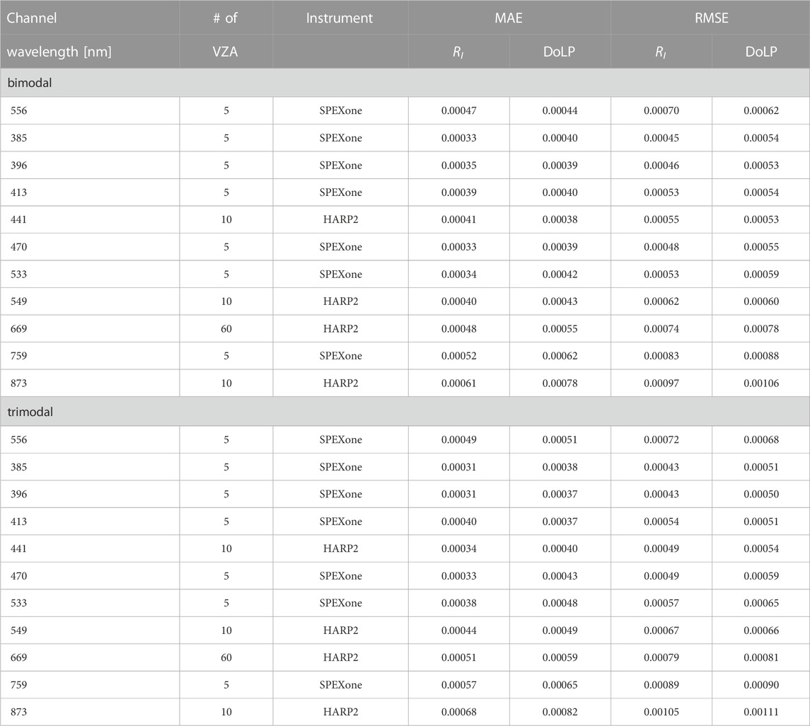
TABLE 1. PACE-MAPP instrument channels, viewing zenith angles, and per-channel performance of the vector radiative transfer model of the neural network. For our study, we assume the 5 SPEXone VZA are 58.07°, 22.65°, 4.42°, −22.66°, −58.07°. For HARP2 we select either 10 or 60 VZAs depending on the channel, with the assumption that they are evenly spaced between −57° and 57°. Channels from OCI will be included in the next version of PACE-MAPP.
3 Retrieval methodology
PACE-MAPP is adapted from the automated and operational RSP Microphysical Aerosol Properties from Polarimetry (RSP-MAPP) retrieval algorithm (Stamnes et al., 2018b). RSP-MAPP was developed for accurate retrieval of aerosol and ocean products for the airborne NASA Goddard Institute for Space Studies Research Scanning Polarimeter (Cairns et al., 1999). An overview of the PACE-MAPP neural network models are depicted in Figure 1. An overview of the PACE-MAPP pre-processing, optimal estimation, and post-processing steps is depicted in Figure 2. The RSP-MAPP algorithm is an automated, operational tool for retrieval of aerosol parameters over oceans that provides aerosol and ocean products for airborne data. Archived data products from RSP-MAPP are available from the following field campaigns: (i) Two-Column Aerosol Project (TCAP, 2012); (ii) Studies of Emissions and Atmospheric Composition, Clouds and Climate Coupling by Regional Surveys (SEAC4RS, 2013); (iii) the Ship-Aircraft Bio-Optical Research (SABOR, 2014); (iv) the North Atlantic Aerosols and Marine Ecosystems Study (NAAMES, 2015–2017); (v) ObseRvations of Aerosols above CLouds and their intEractionS (ORACLES, 2016–2018); (vi) Aerosol Characterization from Polarimeter and Lidar (ACEPOL, 2017); (vii) the Cloud, Aerosol and Monsoon Processes Philippines Experiment (CAMP2Ex, 2019), and (viii) the Aerosol Cloud meTeorology Interactions oVer the western ATlantic Experiment (ACTIVATE, 2020–2022).
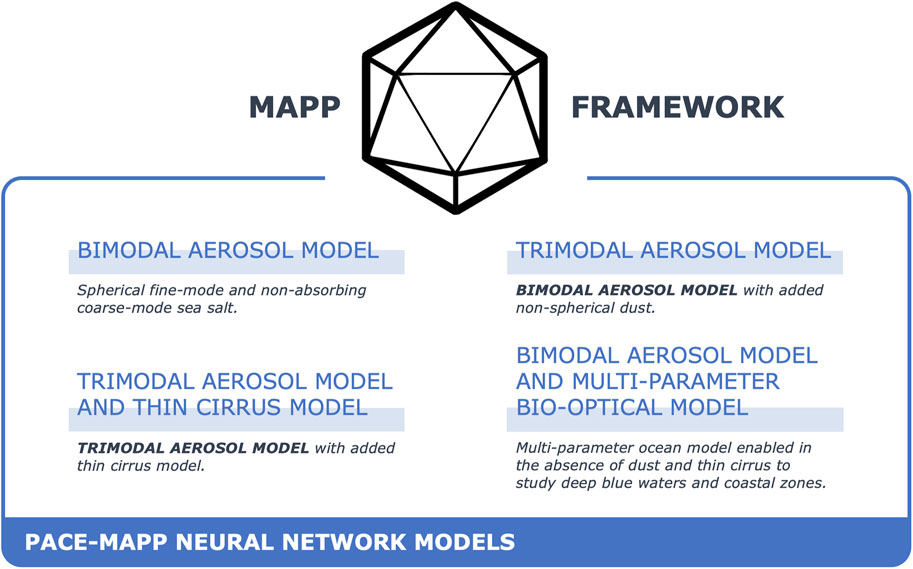
FIGURE 1. The MAPP framework is modular such that researchers can incorporate various neural networks with different aerosol, ocean and cloud models to evaluate which models can provide the best fit to PACE measurements.
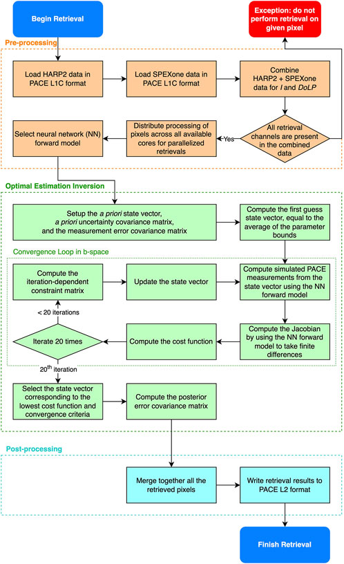
FIGURE 2. PACE-MAPP flow chart of retrieval methodology including the pre-processing, optimal estimation inversion, and post-processing procedures.
3.1 Optimal estimation
The MAPP algorithms use optimal estimation Rodgers (2000) to iteratively find the solution beginning with a first guess to minimize the following cost function:
The vector radiative transfer model is our forward model f, and provides spectrometer-measured intensities that can be expressed as the BRF RI using Eq. 2 and the polarimeter-measured DoLP defined by Eq. 3. f is a function of the state vector x.
3.2 State vector
The state vector contains the aerosol and ocean parameters that define a suitable atmosphere-ocean model for polarimeter measurements y. The aerosol state vector is described in Section 4 and the ocean state vector is described in Section 5 and the full list of state vector parameters are numbered in Table 2. The measurements y can be either real measurements from PACE or synthetic measurements generated by the forward model with noise added. The first term in Eq. 1 may be called the data term since it depends on residuals of the forward model and the measurement, taking into account measurement error through the measurement error covariance matrix Sϵ. The second a priori term is the departure of the state vector x from the a priori state vector xa, with a priori uncertainty provided by the a priori covariance matrix Sa. The prior for each element in the state vector is the mean of the allowable range, and the standard deviation of the uncertainty is also the mean of the allowable range. The full details of the a priori state vector and covariance matrices and the iteration procedure for the MAPP algorithms are provided in Stamnes et al. (2018b).
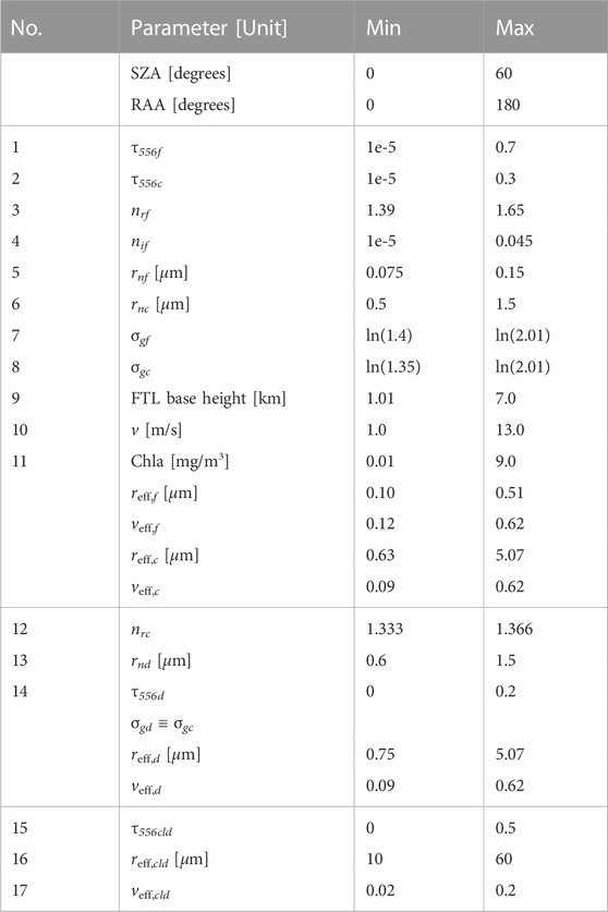
TABLE 2. PACE-MAPP solar-instrument geometry and state vector bounds. Parameter labels f, c, and d denote fine-mode aerosol, coarse-mode sea salt aerosol, and coarse-mode dust aerosol, respectively. τ556 is the optical depth at the wavelength 556 nm. nr and ni are respectively the real and imaginary refractive indices. rn is the median radius. σg is the size distribution width. The wind speed v and Chla are as defined in Section 5. Values are randomly selected from a uniform distribution. τ556 and Chla have half of their values selected from a lognormal distribution. The numbered parameters comprise the state vector. Parameters 1–11 are included in the bimodal aerosol ocean retrieval. Parameters 1–14 are used in the trimodal aerosol retrieval. Parameters 15–17 represent the thin cirrus model that will be added in the next version of PACE-MAPP.
3.3 Forward model
The Earth’s coupled atmosphere-ocean system is fully defined by the complete aerosol and ocean state vector, x. Once we additionally specify the Solar Zenith Angle (SZA) and Relative Azimuth Angle (RAA), a vector radiative transfer program computes the bidirectional reflectance factors (BRFs) RI, RQ, and RU. The BRFs are defined as the I, Q, and U Stokes parameters scaled to be unitless using:
and likewise for the factors RQ and RU. The Stokes parameters I, Q, U have units [W/m2/sr], the solar irradiance E0 has units [W/m2], μ0 is the cosine of the SZA, and π has units [sr]. The DoLP is defined as
This mapping from the input state vector to the output BRF and DoLP at the desired polarimeter channel wavelengths and viewing zenith angles via the vector radiative transfer program represents our forward model.
3.4 Optimal estimation inversion
In nonlinear optimal estimation, we minimize the cost function, Eq. 1, through an iterative process whereby the state vector x is changed until the resulting forward-modeled measurements f(x) match the measurements y within their uncertainties, as outlined in Figure 2. A transformation into b-space is used to smooth out changes between the different state parameters that have different units and ranges, which is similar to a transformation into log-space (Stamnes et al., 2018b). The next step in the iteration is given according to the following equation:
where bi, ba, and Kb represent in b-space the state vector at the ith step, the a priori state vector, and the Jacobian matrix, respectively. The iteration-dependent constraint matrix Si is given by:
where
has constants a0 = 1,000 and b0 = 8 that are determined empirically such that the state vector converges to a solution in an efficient and robust manner (Wu et al., 2017). In practice, we train a neural network to provide the output for our forward model. We take finite differences of this neural network forward model to compute the Jacobian, which we can efficiently compute by consolidating all inputs into a single call to TensorFlow per iteration as described in Section 6.3. Otherwise a complete description of the equations used in the optimal estimation inversion is given in Stamnes et al. (2018b).
4 Aerosol model
The PACE-MAPP aerosol model is either bimodal or trimodal, and thus consists of two (or three) lognormal size distributions that are externally mixed: (i) fine-mode particles are assumed to be spherical, and the fine-mode refractive index is retrieved as independent of wavelength; (ii) coarse-mode sea salt particles are also assumed to be spherical with a fixed complex refractive index corresponding to non-absorbing hydrated sea salt particles; (iii) optionally, for the trimodal aerosol model, non-spherical coarse-mode dust particles are also included. The optical depths of the fine-mode and coarse-mode sea salt are retrieved at the reference wavelength of 556 nm. The fine-mode and coarse-mode sea salt particle effective radii and effective variances are retrieved. The fine-mode real and imaginary refractive indices are also retrieved, the latter of which accounts for aerosol absorption. In the trimodal aerosol model, the free tropospheric layer (FTL) also contains a non-spherical coarse-mode dust aerosol, which has two independent parameters: the dust aerosol optical depth and the dust effective radius. The dust effective variance is assumed to be the same as that of the coarse-mode sea salt, and the spectral complex refractive index of the dust aerosol is fixed according to climatology for the Bahrain AERONET site in the Persian Gulf (Dubovik et al., 2002). For the non-spherical shape of the dust, we assume that the dust is spheroidal with an equiprobable aspect ratio, such that the particles are as equally likely to be oblate as prolate. In the bimodal retrieval, we assume that the real refractive index of sea salt is fixed to a value 1% larger than water, or 1.346 at 556 nm. In the trimodal aerosol retrieval, the sea salt coarse-mode real refractive index is also allowed to vary from that of water for a minimum of ∼1.333 at 556 nm, to a maximum value of 2.5% larger or ∼1.366 at 556 nm.
4.1 Aerosol location
In terms of location, we use a unique structure that places the aerosols in a two-layer system comprised of a marine boundary layer (MBL) and a FTL. Aerosols in the MBL are treated as an external mixture of coarse-mode spherical sea salt and fine-mode aerosols to represent mixing of continental aerosols including pollution and smoke into the MBL. Based on the idea that the bulk of marine aerosol particles is primarily confined to the MBL (Behrenfeld et al., 2019), the FTL consists of spherical fine-mode aerosol particles, with an option to be externally mixed with non-spherical dust particles. We thus assume that the coarse-mode sea salt particles are located in the marine boundary layer between the ocean surface and 0.5 km. The fine-mode aerosol is mixed homogeneously between the surface and 1 km, which is assumed to be the height of the marine boundary layer (MBL). The fine-mode aerosol component is also present in the FTL, which is located at the (retrieved) FTL base height and is assumed to have a physical thickness of 1 km, with a location that can vary between 1 and 8 km. For example, the FTL spans the range of 4–5 km if the FTL base height is 4 km. The trimodal aerosol model adds coarse-mode dust particles that are homogeneously externally mixed with the fine-mode aerosol into the FTL. The fixed physical thickness values that are used for the location of coarse-mode sea salt aerosol (0–0.5 km), the location of the MBL (0–1.0 km) and physical thickness of the FTL (1 km thick) are based on lidar observations over the northern and southern Atlantic ocean, but different average physical thickness heights can be used in different regions of the world. Polarimeter observations are typically found to have a retrieval uncertainty of ∼1 km to aerosol layer height, and are thus not expected to be extremely sensitive to the fixed physical heights of the MBL and FTL compared to the optical depths of the aerosol modes contained within the layers.
4.2 Aerosol state vector
The single-scattering properties of spherical particles are obtained using the highly accurate and freely available Scale Invariance Rule Aerosol Look-Up Table (SIR-A LUT) (Chemyakin et al., 2021). The single-scattering properties of the spheroidal dust particles are computed using the AERONET LUT (Dubovik et al., 2006). The bimodal aerosol parameters included in PACE-MAPP are listed in Table 2 as parameters 1–9. The trimodal aerosol model adds one parameter to fine-tune the water-like real refractive index of the sea salt aerosol (parameter 12), and two parameters to describe coarse-mode dust, which are listed as parameters 13–14. The state vector for our bimodal aerosol model is thus
and the state vector for our trimodal aerosol model is
4.3 Aerosol model summary
This two-layer aerosol system, with up to three distinct aerosol types with different complex refractive indices, provides a realistic representation of aerosol types and location over the open ocean and coastal areas based on goodness of fit to hyperangular polarimeter measurements from 410 to 2,264 nm. The corresponding RSP aerosol and ocean products are publicly available and archived for TCAP, SABOR, NAAMES, ORACLES, CAMP2Ex, and ACTIVATE airborne field campaigns (Stamnes et al., 2018b). The accuracy of the aerosol location parameterization will continue to be validated against aircraft HSRL lidar data since aerosol location directly influences aerosol absorption retrieval accuracy. For particle size, we prefer to use the effective radius and variance since they can be used to describe any aerosol size distribution. We note that PACE-MAPP assumes that the aerosol size distributions are lognormal with a median radius and mode width, and the analytic formulas for effective radius and variance are described in Appendix A.
5 Ocean bio-optical model
PACE-MAPP will adapt two bio-optical models. In this study we use a modified version of the DP-I (Detritus-Plankton) polarized ocean bio-optical model that was originally created for the NASA RSP and APS sensors (Chowdhary et al., 2006; 2012). The coated sphere model has recently been found to result in much more realistic number concentrations for particles, while still yielding realistic hemispherical backscatter values (Organelli et al., 2018). Thus, in addition to this default chlorophyll-based bio-optical model, in the future we plan to further build upon this ocean model by creating a multi-parameter bio-optical model, in which we will upgrade the plankton component from using homogeneous spheres to coated spheres while incorporating wavelength dependent Mie parameters for both the coated sphere plankton and the homogeneous nonalgal particles, as detailed in Section 8. The polarized ocean bio-optical model will be organized as a stand-alone module (PACE-MAPP Module 1) that can be included in other vector radiative transfer codes as part of the boundary condition for the ocean and will be made available to all PACE as well as other interested researchers. Additionally, look-up tables incorporating the full dynamic ranges of Mie parameters for forward modeling of the inherent optical properties for both coated and homogeneous spheres have already been created and will also be made available. The ocean module, together with a Cox-Munk model for ocean surface roughness (Cox and Munk, 1954) and a Lambertian or Fresnel reflectance correction for whitecaps (Koepke, 1984; Frouin et al., 1996), will provide a complete and coupled model for the ocean reflectance, which is numerically efficient and accurate (targeting better than 1% accuracy for the top-of-atmosphere (TOA) I, Q, and U Stokes parameters).PACE-MAPP focuses on the most important first-order effects for the TOA total and polarized radiances, namely, the elastic scattering and absorption by particles in the ocean, and specifically the use of a coated sphere model for phytoplankton. Second-order effects, due to inelastic scattering sources like fluorescence and Raman scattering, are ignored because their influence on the reflectance at TOA is weak (Chowdhary et al., 2019). PACE-MAPP will implement two ocean bio-optical models to represent the ocean which is modeled as pure water with embedded particulate and dissolved impurities. A one-parameter model for the global ocean is chlorophyll-a-based using one parameter, and is based on the DP-I bio-optical model (Chowdhary et al., 2012), which will be denoted as xbio-optical model = [Chla]. This one-parameter ocean bio-optical model is suitable for the Earth’s global ocean and is partially based on empirically-derived relationships for the spectral dependence of the absorption of pigmented particles and the hemispherical backscattering coefficient of the bulk population of particles. A second multi-parameter bio-optical model will be based on a new bio-optical model that we are developing to connect the inherent optical properties of oceanic particles to optical and microphysical properties using a database of coated and uncoated hydrosol single-scattering properties, and will be denoted by the state vector xbio-optical model = xbio-optical model,DP5. This new multi-parameter model is expected to be suitable for complex waters in which current assumptions about the spectral absorption and scattering coefficients are either invalid, or do not follow the empirical models assumed in our global ocean model. PACE-MAPP also retrieves the roughness of the ocean surface, which is modeled using a 1-dimensional Cox-Munk surface (Cox and Munk, 1954). The ocean state vector is thus given by
where v is the wind speed in m/s that determines the ocean surface roughness1.
5.1 Ocean state vector
The PACE-MAPP one-parameter ocean bio-optical model is described by the chlorophyll-a concentration (Chowdhary et al., 2012; Stamnes et al., 2018b) so that the ocean state vector is given by
where [Chla] is the chlorophyll-a concentration in mg/m3. The ocean parameters included in PACE-MAPP are listed in Table 2 as parameters 10–11.
6 PACE-MAPP neural network forward model
The PACE-MAPP neural network forward model is a dense, fully-connected neural network that was trained using TensorFlow 2. Accurate vector radiative transfer codes are slow and computationally intensive, particularly when performing high-accuracy computations using a large number of streams as needed for calculations that include scattering by large oceanic particles or large ice crystal particles found in cirrus clouds. The PACE-MAPP neural network forward model was created to replace the need for online vector radiative transfer calculations by leveraging the tremendous speed improvements achieved by neural networks. The training uses a synthetic dataset (SD) that we created by running a large number of forward model computations with all state vector inputs randomized, where the state vector is discussed in Section 6.1, the details of the neural network training including the SD size are explained in Section 6.2, and a summary of the neural network is provided in Section 6.4. Use of realistic combinations of aerosol and water IOPs that occur in nature would be useful for developing inverse neural networks that can map from TOA radiances directly to the aerosol and ocean state vector. It is also important to ensure that the combinations of water IOPs from the bio-optical models are realistic, and to ensure that the forward model provides a smooth transition from complex coastal environments to simple open ocean environments, as discussed by Fan et al. (2021).
6.1 PACE-MAPP state vector
The state vector of PACE-MAPP retrieval parameters is defined as
where xaerosol is the bimodal (or trimodal) aerosol state vector defined in Section 4 and xocean is the ocean state vector defined in Section 5.We compute the factors RI, RQ, RU at 160 VZA from −65° to 65°, where the negative VZA denotes viewing angles shifted by 180° in azimuth from the positive VZA. The bounds with which the parameters are modeled can be viewed in Table 2. The VZA are generated at 11 channels centered at the 11 channels selected for PACE-MAPP as described in Section 2.
6.2 PACE-MAPP neural network input/output
The PACE-MAPP neural network accepts 14 input parameters using the bimodal aerosol model, which we will refer to as the bimodal PACE-MAPP neural network, or 17 input parameters using the trimodal aerosol model, which we will refer to as the trimodal PACE-MAPP neural network. We label these input parameters as the neural network state vector:
where the cosines of the three solar-instrument observation geometries (SZA, RAA, and VZA) are followed by the state vector x. The PACE-MAPP neural network outputs RI and DoLP for a given atmospheric-ocean state vector and solar-instrument observation geometry. The bimodal PACE-MAPP neural network model maps these 14 input parameters to 22 output values: RI and DoLP at 11 channels at a single VZA. We randomly select 40 VZA between 0° and 65° for every combination of SZA, RAA, and x. For training purposes we note that VZA between 0° and −65°, where the negative value indicates VZA that are viewed by changing the azimuth by 180°, can be obtained by azimuthal symmetry from (180°+ RAA). Very low surface roughness, which occurs rarely over the global ocean but which leads to mirror-like reflection that results in extreme reflectance values that can require additional training to capture, was avoided by removing all cases where the wind speed is less than 1 m/s. For training and validation purposes, the data are split such that 85% of the data is used for training while the remaining 15% is used for validation. This allocation leads to a total of 45,495,680 samples for training and 8,848,320 samples that can be used for validation. Since all of the input and output parameters have different ranges of values, the neural network may become biased to larger numbers. To prevent such biases, we use min-max normalization to scale all values between 0 and 1, defined as
where v is all of a variable’s data, vmin is the smallest value for v, and vmax is the largest value for v. For the training set, the solar-instrument observation geometries, x, and outputs (I and DoLP) are all normalized independently. Using the same normalization values from the training set, the solar-instrument observation geometries and x are also normalized on the validation set.
6.3 PACE-MAPP neural network forward model performance
The performance of the bimodal PACE-MAPP neural network forward model is depicted in Figure 3. The performance of the neural network model for the trimodal aerosol model is similar, and the RMSE and MAE for the both the bimodal and trimodal PACE-MAPP neural network forward models are tabulated in Table 1. The bimodal PACE-MAPP neural network is 25.8 MB in size. Table 3 summarizes how long it takes the bimodal PACE-MAPP neural network to compute the I and DoLP for all 11 channels for varying numbers of viewing zenith angles. The approximate speed to run one forward model simulation for 125 VZA corresponding to combined SPEXone and HARP2 observations is ∼0.045 s. TensorFlow 2 can parallelize multiple inputs so that the performance does not increase linearly. The performance of the neural network scales very well as the number of samples increases. We take advantage of this scaling by noting that we need to call the neural network model multiple times per iteration to find solutions at multiple VZAs and to compute the Jacobian required for optimal estimation retrieval by taking finite differences. The Jacobian thus involves 12 forward model calculations per iteration for the bimodal aerosol model. Since each retrieval uses 20 iterations, there are a total of 12 × 20 = 240 neural network forward model calls including the Jacobian computation. However, by consolidating the calls at multiple angles and the finite difference Jacobian computation into a single call for efficiency, this results in only 20 separate TensorFlow calls per retrieval.

FIGURE 3. PACE-MAPP neural network forward model performance for I and DoLP using the bimodal aerosol model.
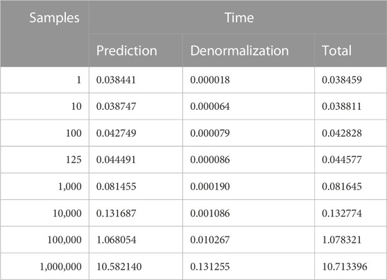
TABLE 3. PACE-MAPP neural network speed. The time, in seconds, to run the bimodal PACE-MAPP neural 4network forward model for different numbers of samples. One sample refers to computing the output corresponding to one input neural network state vector using a single core. Prediction time refers to the amount of time to call the TensorFlow 2 neural network. Denormalization time refers to the amount of time to undo the min-max normalization.
6.4 PACE-MAPP neural network summary
The PACE-MAPP neural network is trained using scientific machine learning, which is distinguished from machine learning in that it is trained to reproduce the results from a scientific model, namely, a vector radiative transfer model. The PACE-MAPP neural network maps from xNN to the output RI and DoLP at 11 channels at a single VZA. However, since we consolidate all the input VZAs and the input perturbations for the Jacobian K into a single TensorFlow call, we efficiently obtain the full RI and DoLP at all requested channels and all VZAs and the corresponding Jacobian K in one pass. The PACE-MAPP neural network is fully connected with an architecture of 14 × 1,024 × 1,024 × 1,024 × 22 and has three dense hidden layers that use the ReLU activation function. For training, the adam optimizer is used in relation to the mean_squared_error loss function. The learning rate is kept fixed at a constant 10–5. Updates to the model are made in batches of 200 samples at a time. Peak model performance for the bimodal aerosol model is achieved after training for 285 epochs.
7 Results
A total of 120,000 simulated retrievals are performed by running the PACE-MAPP forward model with input generated Monte-Carlo-style on samples taken from uniform random distributions for all 11 state parameters using the ranges in Table 2. The solar-instrument geometries are also randomly varied. The actual solar-instrument geometries observed by PACE will not vary randomly, and will have a seasonal dependence, but are not expected to significantly impact aerosol retrieval performance over the ocean. Instrument noise is added as described in Section 2. We select retrievals that have a normalized cost function below 0.05 to represent cases that successfully converge. This convergence filter results in a total of 92,426 successful bimodal cases for a convergence rate of 77%. The resulting scatter-plot of truth vs. retrieved state parameters is depicted in Figure 4 (bimodal) and Figure 5 (trimodal). The performance of the bimodal and trimodal aerosol and ocean retrieval parameters are summarized in Table 4 and generally agree with expectations for aerosol retrievals from the SPEXone instrument (Hasekamp et al., 2019). Choosing the RMSE as an estimate of the 1σ product uncertainty, we find that for bimodal aerosol scenes that we expect to retrieve AOD to ∼0.01, fine-mode AOD to ∼0.02, and coarse-mode AOD to ∼0.01. The total aerosol single-scattering albedo uncertainty at 556 nm, SSA556, is ∼0.01. We expect to retrieve the fine-mode effective radius to ∼0.02 μm, the coarse-mode effective radius to ∼0.29 μm, and the fine- and coarse-mode effective variances to ∼0.06 and ∼0.08, respectively. We expect to retrieve the fine-mode RRI to ∼0.03, and the IRI to ∼0.004, corresponding to a fine-mode SSA556f uncertainty of ∼0.02. The FTL base height is retrieved to ∼0.9 km. Surface slope is retrieved to ∼0.002 corresponding to a wind speed retrieved to ∼0.7 m/s. Chla is retrieved to ∼0.8 mg/m3. Note that these are modeled estimates of the approximate retrieval performance using synthetic measurements using the 11 channels that are sampled at the combined 125 viewing angles we have selected in Table 1. The real-world uncertainties for clear-sky PACE observations over the ocean without thin cirrus will depend on the instrument performance on-orbit, forward model errors, and the availability of suitable a priori information that can be used to help constrain the retrieval. The average time to run one simulated retrieval is ∼4.5 s on a single core of an Intel Gold 6148 Skylake processor. Our objective for processing PACE L1C data files is to enable low latency aerosol, cloud, and ocean product acquisition with an average retrieval speed of ∼1 s per L1C pixel.
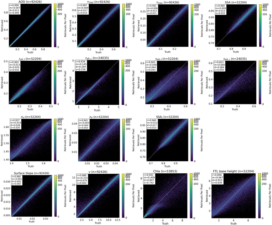
FIGURE 4. PACE-MAPP bimodal aerosol and ocean parameter retrieval performance. The top left corner of each scatter represents the following information: r = R, m = MAE, d = RMSE, and s = STD.
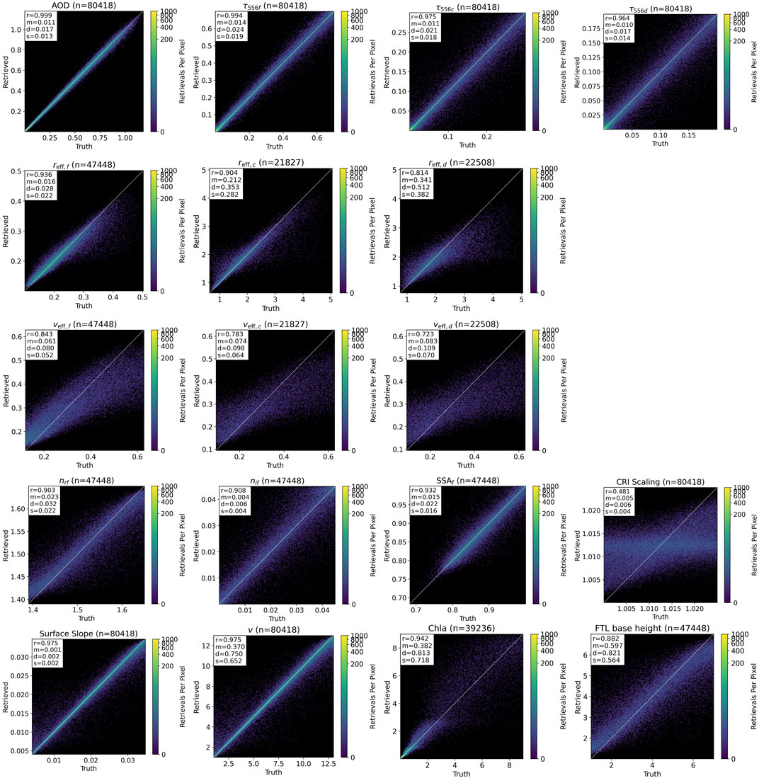
FIGURE 5. PACE-MAPP trimodal aerosol and ocean parameter retrieval performance. The top left corner of each scatter represents the following information: r = R, m = MAE, d = RMSE, and s = STD.
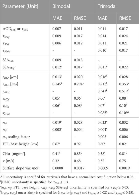
TABLE 4. Simulated PACE-MAPP aerosol and ocean retrieval performance for the bimodal and trimodal aerosol models. Refer to Table 2 for symbol descriptions.
8 Future perspectives
In this section we briefly discuss future planned upgrades. In Section 8.1 we discuss the bio-optical model that uses coated and uncoated hydrosol particles. We discuss the simultaneous retrieval of aerosol and thin cirrus properties in Section 8.2. Other planned upgrades include the use of OCI SWIR channels, some of which must include a retrieval or correction for water vapor, parameterization of the dust complex refractive index using principal component analysis (Wu et al., 2015), increased absorption due to brown carbon aerosol in the UV, deviations in the total pressure thickness of the atmosphere which controls Rayleigh scattering, and the window channel corrections for any minor attenuation due to absorption by gaseous species such as water vapor, nitrogen dioxide, ozone, methane and carbon dioxide.
8.1 Multi-parameter bio-optical model with coated and uncoated hydrosol particles
The coated sphere model has recently been found to result in much more realistic number concentrations for particles, while still yielding realistic hemispherical backscatter values (Organelli et al., 2018). This coated sphere model allows us to develop a biologically-founded mechanistic representation of phytoplankton inherent optical properties, where the coated sphere is modelled with a weakly refractive cytoplasm core surrounded by a much more refractive shell of photosynthetic pigments (Bernard et al., 2009). The incorporation of a bio-optical model that includes coated spheres allows for investigations into how the coated sphere model impacts the results for the aerosol and ocean products compared to a bio-optical model that uses only homogeneous spheres. Depigmented particles are another important oceanic optical constituent that can often vary independently from the chlorophyll-a concentration, particularly in coastal environments. The PACE-MAPP multi-parameter ocean bio-optical model uses a mixture of coated and uncoated hydrosol particles with a Junge particle size distribution. Note that although these coated particles are still spherical particles, rainbow-like features are significantly dampened between scattering angles of 137–165° because the relative real refractive index (RRI) is well below the 1.33 corresponding to cloud droplets in air. And the integration over size is performed using a Junge size distribution that covers over three orders of magnitude of radii values, smoothing out oscillations. Depigmented particles are modeled as uncoated spheres with a radius range between 0.01 and 100 μm, a constant RRI, and an exponentially decaying imaginary refractive index (IRI) with respect to wavelength. Plankton are modeled as coated spheres with a radius range between 0.15 and 100 μm, a fixed core volume ratio (85%), and a weakly refractive core and a more refractive shell relative to that of water (Chemyakin and Stamnes, 2023). Table 5 lists the input Lorenz-Mie parameters covered by our coated and uncoated hydrosol LUTs. These LUTs are expected to be valid across the entire UV-VIS-NIR spectral range for PACE.
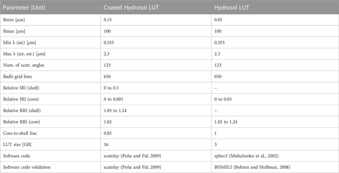
TABLE 5. PACE-MAPP coated and uncoated hydrosol particle LUTs.
8.2 Simultaneous retrieval of thin cirrus properties
Optically thin cirrus is an important issue since current MODIS retrievals have demonstrated biases in aerosol optical thickness due to contamination by thin cirrus clouds (Sun et al., 2011). In fact, any retrieval in which the impact of cirrus has not been carefully considered will likely have cirrus contamination since detecting thin cirrus is difficult with existing detection schemes due to confounding scattering and absorption from aerosols and the surface (e.g., ocean and land). The best way to retrieve thin cirrus properties over the ocean using multi-spectral total and polarized radiance measurements may be using a simultaneous retrieval along with the aerosol and ocean components. Multi-angle polarimetry offers unique sensitivity to thin cirrus as its spectral polarimetric signal differs substantially from the aerosol signals (Sun et al., 2015). We plan to target retrievals of aerosol and ocean properties together with thin cirrus of optical depth 0.5 or less at 670 nm. The aerosol and ocean signal will in general significantly weaken as the cirrus optical depth increases, but also depends on the relative aerosol-to-cirrus loading, the ocean surface roughness, and the ocean subsurface brightness. The three thin cirrus parameters that are expected to be included in PACE-MAPP are listed in Table 2 as parameters 15–17.
9 Conclusion
We have described the development and preliminary performance of PACE-MAPP which retrieves fine- and coarse-mode optical and microphysical properties and the ocean chlorophyll-a concentration and wind speed using both polarimeters and OCI for the PACE mission. The PACE-MAPP algorithm retrieves the following column-averaged total, fine-mode, and coarse-mode ambient aerosol optical and microphysical properties: aerosol optical depth, effective radius, complex refractive index, and aerosol absorption or single-scattering albedo using the total and/or polarized spectral bands from 380–2,260 nm (Mishchenko et al., 2004; Chowdhary et al., 2005; Stamnes et al., 2018b). The vector radiative transfer model used in PACE-MAPP treats the ocean surface roughness by using the wind speed to parameterize the ocean surface facets and includes coupling to the ocean subsurface parameterized by the chlorophyll-a concentration (Chowdhary et al., 2006; 2012), and an upgraded multi-parameter bio-optical model that will be used for coastal waters which cannot be described adequately by a one-parameter model. The PACE-MAPP aerosol LUTs and the coated and uncoated hydrosol LUTs and bio-optical model are available for free download and assessment by the community. Future work will involve training neural networks that include the complex ocean bio-optical model for coastal zones, non-spherical coarse-mode dust aerosol and thin cirrus clouds, and to compute the water-leaving radiance using the retrieved aerosol-ocean state vector. One objective of the improved bio-optical model is to allow for a smooth transition from open ocean water to complex coastal environments as described by Fan et al. (2021). In addition to the performance on simulated data presented here, in the future the PACE-MAPP retrieval algorithm can be tested with airborne PACE-like data collected during the SABOR, NAAMES, and ACEPOL campaigns, and the future ACTIVATE dataset. Validation of the ocean retrieval products from airborne RSP, SPEXairborne, and AirHARP will be accomplished using ship-based in situ measurements and collocated High Spectral Resolution Lidar (HSRL) (Hair et al., 2008) ocean measurements. Validation of the aerosol retrieval products will be accomplished via HSRL aerosol measurements and AERONET station overpass comparisons. The PACE-MAPP retrieval algorithm will be robust so that it will have the capability to provide improved results for aerosol and ocean products data as long as either SPEXone or HARP2 is operational, by combining data from a single polarimeter with the OCI SWIR channels, or using only data from both the polarimeters without the OCI SWIR channels. PACE-MAPP is extremely fast due to the incorporation of neural networks into its framework, which is expected to make its products suitable for low-latency applications such as weather forecasting and air quality monitoring.
Data availability statement
Publicly available datasets were analyzed in this study. This data can be found here: The aerosol and hydrosol scale-invariant rule LUTs are publicly available for download at https://science.larc.nasa.gov/polarimetry/. Results from the MAPP algorithm for RSP are available from the NASA Langley Airborne Science Data archive at https://www-air.larc.nasa.gov/ and the NASA GISS RSP website at https://data.giss.nasa.gov/pub/rsp/.
Author contributions
Algorithm development: SS, MJ, AB, EC, and BC. All authors contributed to the article and approved the submitted version.
Funding
This work was funded by the NASA PACE mission.
Conflict of interest
Authors EC and MJ were employed by Science Systems and Applications, Inc.
The remaining authors declare that the research was conducted in the absence of any commercial or financial relationships that could be construed as a potential conflict of interest.
Publisher’s note
All claims expressed in this article are solely those of the authors and do not necessarily represent those of their affiliated organizations, or those of the publisher, the editors and the reviewers. Any product that may be evaluated in this article, or claim that may be made by its manufacturer, is not guaranteed or endorsed by the publisher.
Footnotes
1Although we use “wind speed” as our retrieval parameter, strictly speaking we are sensitive to and retrieve the variance of the probability distribution of facet slopes, which is proportional to the wind speed through the relation facet surface slope variance = 0.0015 + 0.00256v.
References
Behrenfeld, M. J., Moore, R. H., Hostetler, C. A., Graff, J., Gaube, P., Russell, L. M., et al. (2019). The North atlantic aerosol and marine ecosystem study (NAAMES): Science motive and mission overview. Front. Mar. Sci. 6, 00122. doi:10.3389/fmars.2019.00122
Bernard, S., Probyn, T., and Quirantes, A. (2009). Simulating the optical properties of phytoplankton cells using a two-layered spherical geometry. Biogeosciences Discuss. 6, 1497–1563.
Bohren, C. F., and Huffman, D. R. (2008). Absorption and scattering of light by small particles. United States: John Wiley and Sons.
Cairns, B., Russell, E. E., and Travis, L. D. (1999). “Research scanning polarimeter: Calibration and ground-based measurements,” in SPIE’s international symposium on optical science, engineering, and instrumentation (United States: International Society for Optics and Photonics), 186–196.
Chemyakin, E., Stamnes, S., Burton, S. P., Liu, X., Hostetler, C., Ferrare, R., et al. (2021). Improved Lorenz-Mie look-up table for lidar and polarimeter retrievals. Front. Remote Sens. 2, 711106. doi:10.3389/frsen.2021.711106
Chemyakin, E., Stamnes, S., Hair, J., Burton, S. P., Bell, A., Hostetler, C., et al. (2023). Efficient single-scattering look-up table for lidar and polarimeter water cloud studies. be Submitt. Opt. Lett. 48, 13. doi:10.1364/ol.474282
Chowdhary, J., Cairns, B., Mishchenko, M. I., Hobbs, P. V., Cota, G. F., Redemann, J., et al. (2005). Retrieval of aerosol scattering and absorption properties from photopolarimetric observations over the ocean during the clams experiment. J. Atmos. Sci. 62, 1093–1117. doi:10.1175/jas3389.1
Chowdhary, J., Cairns, B., and Travis, L. D. (2006). Contribution of water-leaving radiances to multiangle, multispectral polarimetric observations over the open ocean: Bio-optical model results for case 1 waters. Appl. Opt. 45, 5542–5567. doi:10.1364/ao.45.005542
Chowdhary, J., Cairns, B., Waquet, F., Knobelspiesse, K., Ottaviani, M., Redemann, J., et al. (2012). Sensitivity of multiangle, multispectral polarimetric remote sensing over open oceans to water-leaving radiance: Analyses of RSP data acquired during the MILAGRO campaign. Remote Sens. Environ. 118, 284–308. doi:10.1016/j.rse.2011.11.003
Chowdhary, J., Zhai, P., Boss, E., Dierssen, H. M., Frouin, R. J., Ibrahim, A. I., et al. (2019). Modeling atmosphere-ocean radiative transfer: A pace mission perspective. Front. Earth Sci. 7, 100. doi:10.3389/feart.2019.00100
Cox, C., and Munk, W. (1954). Measurement of the roughness of the sea surface from photographs of the Sun’s glitter. JOSA 44, 838–850. doi:10.1364/josa.44.000838
Dubovik, O., Holben, B., Eck, T. F., Smirnov, A., Kaufman, Y. J., King, M. D., et al. (2002). Variability of absorption and optical properties of key aerosol types observed in worldwide locations. J. Atmos. Sci. 59, 590–608. doi:10.1175/1520-0469(2002)059<0590:voaaop>2.0.co;2
Dubovik, O., Sinyuk, A., Lapyonok, T., Holben, B. N., Mishchenko, M. I., Yang, P., et al. (2006). Application of spheroid models to account for aerosol particle nonsphericity in remote sensing of desert dust. J. Geophys. Res. 111, D11208. doi:10.1029/2005jd006619
Fan, C., Fu, G., Di Noia, A., Smit, M., Hh Rietjens, J., A Ferrare, R., et al. (2019). Use of a neural network-based ocean body radiative transfer model for aerosol retrievals from multi-angle polarimetric measurements. Remote Sens. 11, 2877. doi:10.3390/rs11232877
Fan, Y., Li, W., Chen, N., Ahn, J.-H., Park, Y.-J., Kratzer, S., et al. (2021). Oc-smart: A machine learning based data analysis platform for satellite Ocean Color sensors. Remote Sens. Environ. 253, 112236. doi:10.1016/j.rse.2020.112236
Fernandez Borda, R., Martins, J., McBride, B., Remer, L., and Barbosa, H. (2018). “Capabilities of the harp2 polarimetric sensor on the pace satellite,” in AGU fall meeting abstracts (Cambridge, MA: Harvard University), 2018. OS11D–1431.
Frouin, R., Schwindling, M., and Deschamps, P.-Y. (1996). Spectral reflectance of sea foam in the visible and near-infrared: In situ measurements and remote sensing implications. J. Geophys. Res. Oceans 101, 14361–14371. doi:10.1029/96jc00629
Gao, M., Franz, B. A., Knobelspiesse, K., Zhai, P.-W., Martins, V., Burton, S., et al. (2021). Efficient multi-angle polarimetric inversion of aerosols and ocean color powered by a deep neural network forward model. Atmos. Meas. Tech. 14, 4083–4110. doi:10.5194/amt-14-4083-2021
Gao, M., Zhai, P.-W., Franz, B., Hu, Y., Knobelspiesse, K., Werdell, P. J., et al. (2018). Retrieval of aerosol properties and water-leaving reflectance from multi-angular polarimetric measurements over coastal waters. Opt. express 26, 8968–8989. doi:10.1364/oe.26.008968
Gordon, H. R. (1997). Atmospheric correction of ocean color imagery in the Earth observing system era. J. Geophys. Res. Atmos. 102, 17081–17106. doi:10.1029/96jd02443
Gorman, E. T., Kubalak, D. A., Patel, D., Mott, D. B., Meister, G., Werdell, P. J., et al. (2019). “The nasa plankton, aerosol, cloud, ocean Ecosystem (pace) mission: An emerging era of global, hyperspectral Earth system remote sensing,” in Sensors, systems, and next-generation satellites XXIII (United States: International Society for Optics and Photonics), 11151, 111510G.
Hair, J., Hostetler, C., Cook, A., Harper, D., Ferrare, R., Mack, T., et al. (2008). Airborne high spectral resolution lidar for profiling aerosol optical properties. Appl. Opt. 47, 6734–6752. doi:10.1364/ao.47.006734
Hansen, J. E., and Travis, L. D. (1974). Light scattering in planetary atmospheres. Space Sci. Rev. 16, 527–610. doi:10.1007/bf00168069
Hasekamp, O. P., Fu, G., Rusli, S. P., Wu, L., Di Noia, A., aan de Brugh, J., et al. (2019). Aerosol measurements by SPEXone on the NASA PACE mission: Expected retrieval capabilities. J. Quantitative Spectrosc. Radiat. Transf. 227, 170–184. doi:10.1016/j.jqsrt.2019.02.006
Hasekamp, O. P., Litvinov, P., and Butz, A. (2011). Aerosol properties over the ocean from parasol multiangle photopolarimetric measurements. J. Geophys. Res. Atmos. 116, D14204. doi:10.1029/2010jd015469
Knobelspiesse, K. D., Bailey, S., Cairns, B., Franz, B. A., Gales, J. M., Gao, M., et al. (2020). “Development of a common level-1c product to facilitate multi-sensor science from the nasa pace mission,” in AGU fall meeting abstracts (Cambridge, MA: Harvard University), 2020. A091–0005.
Koepke, P. (1984). Effective reflectance of oceanic whitecaps. Appl. Opt. 23, 1816–1824. doi:10.1364/ao.23.001816
Mishchenko, M. I., Travis, L. D., and Lacis, A. A. (2002). Scattering, absorption, and emission of light by small particles. United Kingdom: Cambridge University Press.
Mishchenko, M. I., Videen, G., Babenko, V. A., Khlebtsov, N. G., and Wriedt, T. (2004). T-Matrix theory of electromagnetic scattering by particles and its applications: A comprehensive reference database. J. Quant. Spectrosc. Radiat. Transf. 88, 357–406.
Nied, J., Jones, M., Seaman, S., Shingler, T., Hair, J. W., Cairns, B., et al. (2023). A cloud detection neural network for above-aircraft clouds using airborne cameras. Front. Remote Sens. 4, 12. doi:10.3389/frsen.2023.1118745
Organelli, E., Dall’Olmo, G., Brewin, R. J., Tarran, G. A., Boss, E., and Bricaud, A. (2018). The open-ocean missing backscattering is in the structural complexity of particles. Nat. Commun. 9, 5439. doi:10.1038/s41467-018-07814-6
Peña, O., and Pal, U. (2009). Scattering of electromagnetic radiation by a multilayered sphere. Comput. Phys. Commun. 180, 2348–2354. doi:10.1016/j.cpc.2009.07.010
Rietjens, J. H., Campo, J., Smit, M., Winkelman, R., Nalla, R., Landgraf, J., et al. (2021). “Optical and system performance of spexone, a multi-angle channeled spectropolarimeter for the nasa pace mission,” in International conference on space optics—icso 2020 (United States: International Society for Optics and Photonics), 11852, 1185234.
Stamnes, K., Li, W., Yan, B., Eide, H., Barnard, A., Pegau, W., et al. (2003). Accurate and self-consistent Ocean Color algorithm: Simultaneous retrieval of aerosol optical properties and chlorophyll concentrations. Appl. Opt. 42, 939–951. doi:10.1364/ao.42.000939
Stamnes, S., Baize, R., Bontempi, P., Cairns, B., Chemyakin, E., Choi, Y.-J., et al. (2021). Simultaneous aerosol and ocean properties from the polcube cubesat polarimeter. Front. Remote Sens. 2, 19. doi:10.3389/frsen.2021.709040
Stamnes, S., Fan, Y., Chen, N., Li, W., Tanikawa, T., Lin, Z., et al. (2018a). Advantages of measuring the q Stokes parameter in addition to the total radiance i in the detection of absorbing aerosols. Front. Earth Sci. 6, 34. doi:10.3389/feart.2018.00034
Stamnes, S., Hostetler, C., Ferrare, R., Burton, S., Liu, X., Hair, J., et al. (2018b). Simultaneous polarimeter retrievals of microphysical aerosol and ocean color parameters from the “mapp” algorithm with comparison to high-spectral-resolution lidar aerosol and ocean products. Appl. Opt. 57, 2394–2413. doi:10.1364/ao.57.002394
Stap, F., Hasekamp, O., and Roeckmann, T. (2015). Sensitivity of PARASOL multi-angle photopolarimetric aerosol retrievals to cloud contamination. Atmos. Meas. Tech. 8, 1287–1301. doi:10.5194/amt-8-1287-2015
Sun, W., Baize, R. R., Videen, G., Hu, Y., and Fu, Q. (2015). A method to retrieve super-thin cloud optical depth over ocean background with polarized sunlight. Atmos. Chem. Phys. 15, 11909–11918. doi:10.5194/acp-15-11909-2015
Sun, W., Videen, G., Kato, S., Lin, B., Lukashin, C., and Hu, Y. (2011). A study of subvisual clouds and their radiation effect with a synergy of ceres, modis, calipso, and airs data. J. Geophys. Res. Atmos. 116. doi:10.1029/2011jd016422
van Amerongen, A., Rietjens, J., Campo, J., Dogan, E., Dingjan, J., Nalla, R., et al. (2019). “Spexone: A compact multi-angle polarimeter,” in International conference on space optics—icso 2018 (United States: International Society for Optics and Photonics), 11180, 111800L.
Waluschka, E., Collins, N. R., Cook, W. B., Gorman, E. T., Hilton, G. M., Knuble, J. J., et al. (2021). “Pace ocean color instrument polarization testing and results,” in Earth observing systems XXVI (United States: International Society for Optics and Photonics), 11829, 118290R.
Wu, L., Hasekamp, O., Van Diedenhoven, B., and Cairns, B. (2015). Aerosol retrieval from multiangle multispectral photopolarimetric measurements: Importance of spectral range and angular resolution. Atmos. Meas. Tech. 8, 2625–2638. doi:10.5194/amt-8-2625-2015
Wu, W., Liu, X., Zhou, D. K., Larar, A. M., Yang, Q., Kizer, S. H., et al. (2017). The application of PCRTM physical retrieval methodology for IASI cloudy scene analysis. IEEE Trans. Geoscience Remote Sens. 55, 5042–5056. doi:10.1109/tgrs.2017.2702006
Appendix A: Effective radius and variance
The median radius and mode width are related to the effective radius and variance through the following analytic formulas. For the fine (index f) and coarse (index c) modes we can obtain the effective radius from
and the effective variance as
where rn [μm] is the median radius in number-density space. The median radius is defined as the radius above which there are as many particles as there are particles with radii below rn. The term σg is the size distribution width. For the total size distribution, the effective radius is equal to three times the volume divided by the surface concentration, and can also be written in terms of moments of the size distribution as follows (Hansen and Travis, 1974)
where Vj is the volume concentration [μm3/cm3] and Sj is the surface-area concentration [μm2/cm3]. mk is the kth moment defined by
Keywords: vector radiative transfer, multiple scattering, passive remote sensing, polarimetry, aerosol detection, oceanic optics, neural network
Citation: Stamnes S, Jones M, Allen JG, Chemyakin E, Bell A, Chowdhary J, Liu X, Burton SP, Van Diedenhoven B, Hasekamp O, Hair J, Hu Y, Hostetler C, Ferrare R, Stamnes K and Cairns B (2023) The PACE-MAPP algorithm: Simultaneous aerosol and ocean polarimeter products using coupled atmosphere-ocean vector radiative transfer. Front. Remote Sens. 4:1174672. doi: 10.3389/frsen.2023.1174672
Received: 26 February 2023; Accepted: 19 April 2023;
Published: 11 May 2023.
Edited by:
Jason Xuan, Virginia Tech, United StatesReviewed by:
Weizhen Hou, Harvard University, United StatesXiaoguang Xu, University of Maryland, Baltimore County, United States
Copyright © 2023 Stamnes, Jones, Allen, Chemyakin, Bell, Chowdhary, Liu, Burton, Van Diedenhoven, Hasekamp, Hair, Hu, Hostetler, Ferrare, Stamnes and Cairns. This is an open-access article distributed under the terms of the Creative Commons Attribution License (CC BY). The use, distribution or reproduction in other forums is permitted, provided the original author(s) and the copyright owner(s) are credited and that the original publication in this journal is cited, in accordance with accepted academic practice. No use, distribution or reproduction is permitted which does not comply with these terms.
*Correspondence: Snorre Stamnes, c25vcnJlLmEuc3RhbW5lc0BuYXNhLmdvdg==; Michael Jones, bWljaGFlbC5qb25lcy00QG5hc2EuZ292