Leveraging multimission satellite data for spatiotemporally coherent cyanoHAB monitoring

Cyanobacteria harmful algal blooms (cyanoHABs) present a critical public health challenge for aquatic resource and public health managers. Satellite remote sensing is well-positioned to aid in the identification and mapping of cyanoHABs and their dynamics, giving freshwater resource managers a tool for both rapid and long-term protection of public health. Monitoring cyanoHABs in lakes and reservoirs with remote sensing requires robust processing techniques for generating accurate and consistent products across local and global scales at high revisit rates. We leveraged the high spatial and temporal resolution chlorophyll-a (Chla) and phycocyanin (PC) maps from two multispectral satellite sensors, the Sentinel-2 (S2) MultiSpectral Instrument (MSI) and the Sentinel-3 (S3) Ocean Land Colour Instrument (OLCI) respectively, to study bloom dynamics in Utah Lake, United States, for 2018. We used established Mixture Density Networks (MDNs) to map Chla from MSI and train new MDNs for PC retrieval from OLCI, using the same architecture and training dataset previously proven for PC retrieval from hyperspectral imagery. Our assessment suggests lower median uncertainties and biases (i.e., 42% and -4%, respectively) than that of existing top-performing PC algorithms. Additionally, we compared bloom trends in MDN-based PC and Chla products to those from a satellite-derived cyanobacteria cell density estimator, the cyanobacteria index (CI-cyano), to evaluate their utility in the context of public health risk management. Our comprehensive analyses indicate increased spatiotemporal coherence of bloom magnitude, frequency, occurrence, and extent of MDN-based maps compared to CI-cyano and potential for use in cyanoHAB monitoring for public health and aquatic resource managers.

1 Introduction

Cyanobacteria have been on the planet for over 3 billion years (Schopf, 2002; Paerl & Huisman, 2009) and are ubiquitous in nearly all freshwater environments (Chorus & Welker, 2021). Their ability to adapt to changing environmental, meteorological, and landscape conditions has allowed them to not only survive, but also thrive in the face of climate change and anthropogenic pressures, such as dam construction, deforestation, watershed urbanization, and increasing agricultural activities (Paerl & Huisman, 2009; Nwankwegu et al., 2019). Through a variety of triggers and environmental drivers (Hudnell, 2008), and in conjunction with the cyanotoxins produced by specific cyanobacteria species (Davis et al., 2019), these prokaryotic organisms can proliferate at a high rate across freshwater lakes, reservoirs, ponds, and streams and cause what are colloquially known as cyanobacteria harmful algal blooms (cyanoHABs). Similar to freshwater eukaryotic algal blooms, cyanoHABs can disrupt ecosystem functions and negatively impact water quality through changes in turbidity, dissolved oxygen, and aquatic food webs (Šulčius et al., 2017). However, what distinguishes cyanoHABs in being distinctly more dangerous from their eukaryotic counterparts is the production of cyanotoxins (Rantala et al., 2004).

Cyanotoxins are produced by many, but not all, cyanobacteria species (Salmaso et al., 2016) and pose a significant health risk to humans and animals that come into contact with them (Chorus & Welker, 2021). CyanoHABs may be increasing in frequency and magnitude globally (Oliver et al., 2017; Ho & Michalak, 2020; Coffer et al., 2021; Plaas & Paerl, 2021) and are a critical public health challenge for aquatic resource managers, drinking water utilities, and agricultural communities who rely on surface water as an essential resource. National and world health agencies, such as the U.S. Environmental Protection Agency (US EPA) and World Health Organization (WHO), provide guidance on monitoring, sampling, analysis, and management related to cyanoHABs (World Health Organization, 2003; USEPA, 2019; Chorus & Welker, 2021). For example, the WHO recommends sampling and acting upon both cyanotoxin concentration and cyanobacteria biomass and provides qualitative and quantitative thresholds for when management interventions should be considered (Chorus & Welker, 2021). In order to protect public health and act upon recommended health guidelines, managers must first be able to characterize short- and long-term risk for a given waterbody or cyanoHAB event. The presence and quantification of cyanotoxins and toxigenic cyanobacteria can be determined and measured both in the field with rapid assays (Aranda-Rodriguez et al., 2015) and water quality sensors (Bowling et al., 2016) and with laboratory methods after field sample collection (Mountfort et al., 2005; MacKeigan et al., 2022). Most often, a suite of multiple methods are employed by managers and scientists to best protect the public from cyanoHABs and potential illnesses (USEPA, 2019).

The broad purpose of this study is to advance the quality of satellite-derived cyanobacteria biomass that can reliably assess cyanoHAB risk so that aquatic resource and public health managers have the most spatiotemporally coherent picture of a cyanoHAB event on a given day, season, or across years, allowing them to balance public health and aquatic resource protection with other stakeholder pressures. More specifically, this study has several research objectives, ranging from algorithm development to risk management applicability. First, we aimed to develop and test a mixture density network (MDN) model for phycocyanin (PC) estimation (hereafter MDN-PC) (O’Shea et al., 2021) from images of the Ocean and Land Colour Instrument (OLCI) aboard the Sentinel-3 (S3) mission. This model was trained with in situ data from a variety of freshwater aquatic ecosystems and applied to OLCI images over Utah Lake, United States in the year 2018. Once our PC model was applied to Utah Lake, in the absence of direct PC in situ matchups, we analyzed the quality of our satellite-derived PC products and time series against in situ cell density matchups and the Cyanobacteria Assessment Network (CyAN) maps generated using the cyanobacteria index (CI-cyano) (Schaeffer et al., 2015; Schaeffer et al., 2018). Our third objective was to assess how our MDN-PC model could help to better characterize recreational risk assessment from daily cyanoHABs in a spatiotemporally coherent manner. We did this through both spatial and temporal comparisons of our maps of cyanobacteria biomass estimations of PC to both in situ values and CI-cyano maps through the lens of WHO risk assessment categories for a lake-wide, season-long cyanoHAB that occurred on Utah Lake in 2018. Lastly, we explored the use of machine-learning-derived chlorophyll a (Chla) from the Sentinel-2 (S2) MultiSpectral Instrument (MSI) imagery in conjunction with OLCI-derived PC products with the goal of augmenting spatiotemporal risk assessment in areas such as marinas and beaches that OLCI data cannot reliably capture due to constraints in spatial resolution.

2 CyanoHAB sampling and analysis

2.1 Cyanotoxins

Both cyanotoxins and cyanobacteria abundance can be used independently or together to estimate the magnitude and associated public health risk of a cyanoHAB. Currently, the most reliable and consistent methods for estimating sampled cyanotoxins occur in the laboratory using methods such as enzyme-linked immunosorbent assays (ELISA) or liquid chromatography triple quadrupole mass spectrometry (LC/MS) (Graham et al., 2010; Loftin et al., 2016). There are also several rapid assay test kits available to detect the presence of cyanotoxins in water that can be performed in the field while sampling a bloom, providing results in minutes. While these rapid test kits can provide quick data turnaround and yield sample prioritization for laboratory analysis, they rely on visual (qualitative) assessment for interpreted quantitation, have high false positive rates, and can be relatively costly (Humpage et al., 2012; Aranda-Rodriguez et al., 2015). Field and laboratory analyses of cyanotoxins in discrete spatial and temporal samples only reflect one piece of the puzzle when evaluating the continuous public health risk for a given waterbody. For example, several common cyanotoxins, such as the neurotoxin anatoxin-a, undergo swift degradation in sunlight, with a half-life of fewer than 2 h in ambient environmental conditions (Stevens & Krieger, 1991; USEPA, 2015), and if field sampling occurs after degradation in one location, cyanotoxin exposure risk for the entire waterbody may be underestimated or mischaracterized. Additionally, the exact environmental conditions in which cyanobacteria cells become toxigenic is still unclear (Boopathi & Ki, 2014), therefore there may be a future risk of cyanotoxin production even if toxins are not detected within a bloom at any given point in time or space (Maske et al., 2010). Adding an estimation of cyanobacteria abundance to sampling and decision-making criteria allows for a more comprehensive evaluation of bloom characteristics and evaluated public health risk.

2.2 Cyanobacteria abundance

Augmenting cyanoHAB monitoring with spatial and temporal cyanobacteria abundance estimation not only allows for a direct link to evaluate cyanotoxin exposure risk through known relationships between toxigenic cyanobacteria cell densities and associated cyanotoxins (Pilotto et al., 1997), but also helps characterize how the bloom may be changing in magnitude, extent, and location. Unlike cyanotoxins, there are many methods of estimating cyanobacteria abundance at different spatial, temporal, accuracy, and precision scales. Similar to cyanotoxins, cyanobacteria abundance and taxonomy can be measured in the lab or in the field. Beyond traditional microscope-based manual species identification and cell enumeration, a common laboratory technique includes digital imaging flow cytometry, in which a flow cytometer captures images of individual cells and then compares and matches them to a database for digital image analysis (Sieracki et al., 1998; Buskey & Hyatt, 2006; Sosik & Olson, 2007). Newer laboratory methods, such as qPCR, utilize gene-based approaches to quantify how many toxin-producing cyanobacteria cells exist within a given sample, allowing for more accurate and precise characterization of bloom toxicity and risk (Pinto et al., 2012; Fortin et al., 2015).

In the absence of direct cyanobacteria cell density enumeration in the laboratory, proxy measurements of algal pigments have been shown to be both cost-effective and accurate measures of cyanobacteria abundance. These proxy metrics include measurements of cyanobacteria cell pigments Chla (Loftin et al., 2016) and PC (Brient et al., 2008). Like other photosynthetic organisms, cyanobacteria contain Chla; however, unlike their eukaryotic counterparts, freshwater cyanobacteria also contain significant quantities of phycocyanin (Tandeau de Marsac, 2003; Chorus & Welker, 2021). To estimate cyanobacteria biomass, both pigments can be measured in the lab and in the field through fluoroscopy and spectrometry, with phycocyanin providing a more accurate representation of cyanobacteria abundance within a mixed assemblage of phytoplankton (Brient et al., 2008; Yoshikawa & Belay, 2008; Loftin et al., 2016; Hodges et al., 2018). Using pigment analysis, hand-held sondes, and autonomous, high-frequency sondes on buoys can help characterize cyanoHABs at a larger spatiotemporal scale, yet still lack the ability to fully map a cyanoHAB in its spatial and temporal entirety.

2.3 Optical remote sensing

According to the fundamentals of aquatic optics, the optical properties of pigments and their concentrations, together with other optically relevant materials present in the water column, govern the shape and magnitude of spectral water-leaving radiance (L_w) that can be measured with field-based or space-borne spectro-radiometers (Mobley, 1994; Bukata et al., 1995). Satellite remote sensing is hence well-positioned to aid in the identification and understanding of cyanoHABs and their dynamics over time (Dekker et al., 1996; Kutser, 2004; Simis et al., 2005), giving freshwater aquatic resource managers a complementary tool for both rapid and long-term protection of public health. This has been made possible by examining characteristic spectral features of phycocyanin (i.e., absorption peak ∼620 and fluorescence signature ∼650 nm) that manifest in L_w. Recently, there have been several open-source tools developed to continuously identify and track cyanoHABs and other algal blooms with remote sensing satellite data, including the CyAN (Schaeffer et al., 2018), EOLakeWatch (Binding et al., 2021), and CyanoTRACKER (Mishra et al., 2020); all allowing aquatic managers to track blooms and/or estimate cyanobacteria abundance across large geographic areas and through time—services invaluable to many agencies that do not have the resources to regularly sample for cyanotoxins or cell densities in order to protect public health. These satellite-based cyanoHAB tracking web interfaces use a variety of proxy measurements and algorithms to monitor and track blooms across time.

2.3.1 Chla estimation

Chla, which is common to all phytoplankton types and can be approximated from satellite-derived L_w (Gitelson et al., 2007; O’Reilly & Werdell, 2019), has been the most widely used proxy pigment to study and monitor trophic state (Hu et al., 2004) or cyanoHABs (Park et al., 2010). Chla has been used to monitor cyanoHABs on satellite missions such as Landsat, MEdium Resolution Imaging Spectrometer (MERIS), MODerate Resolution Imaging Spectroradiometer (MODIS), MSI, and OLCI.

With both in situ sensors and well developed laboratory methods for Chla quantification (Sartory & Grobbelaar, 1984), some studies and applications are able to utilize empirical and semi-empirical models to correlate Chla field measurements directly to remote sensing reflectance (R_rs), defined as the ratio of L_w and downwelling irradiance (E_d) just above the water (Mobley, 1999), for robust analysis and Chla estimations (Moses et al., 2009). However, while empirical models may perform well in the specific area or waterbody that in situ data were collected, they tend to perform poorly when applied across waters of differing conditions (Lee et al., 2002). If Chla retrieval algorithms are developed for application across multiple sensors, different locations, and waters with differing optical properties, analytical and semi-analytical models often perform better than locally/regionally empirical models by first deriving the absorption and backscattering properties of water and its constituents from R_rs (Werdell et al., 2018) and subsequently predicting Chla (Moses et al., 2009).

Historically, based on the broadly defined water-type classification, i.e., case I versus case II (Mobley et al., 2004), different retrieval algorithms use different band ratios and combinations. For example, the Maximum Chlorophyll Index (MCI) (Gower et al., 2005), a three-band algorithm that uses the amplitude of the spectral reflectance curves of three red through NIR bands to predict Chla, performs best in productive or eutrophic waters (Binding et al., 2013). Similarly, a study by Chen et al. (2011) demonstrated that a three-band model can effectively estimate Chla concentration in turbid and productive waters, particularly as the concentration increases. Another example is the normalized difference chlorophyll index (NDCI) (Mishra & Mishra, 2012), which is a simpler, two-band ratio to estimate Chla that uses red and NIR spectra and assumes that absorption in the red spectra is dominated by phytoplankton, and absorption in the NIR spectra is dominated by pure water absorption (Dall’Olmo & Gitelson, 2005). The blue-green band ratio is another proxy that has been employed to estimate Chla, but performs poorly in optically complex waters (Le et al., 2013). To help further inform cyanoHAB management decisions, some studies take the satellite-based estimation of Chla and link it directly to absolute values of cyanoHAB abundance, which can then be used by managers to evaluate cyanotoxin exposure risk. This can be done through absolute Chla estimations (mg m⁻³) (Matthews et al., 2012; Moradi, 2014; Palmer et al., 2015) or cyanobacteria cell density (cells mL⁻¹) (Hunter et al., 2010; Wynne et al., 2010; Stumpf et al., 2012; Lunetta et al., 2015).

Despite its historic value and a breadth of options in band combinations and algorithms, there are several issues with using Chla for monitoring cyanoHABs in aquatic environments outside of spectral consistency across waterbodies. The major concern comes from the conflation of the spectral signature of non-toxic eukaryotic phytoplankton, which also displays high Chla values, with the spectral signature of cyanoHABs (Stumpf et al., 2016). In a best-case scenario for the use of Chla for monitoring cyanoHABs, bloom biomass would be composed either entirely or predominantly by toxic cyanobacteria, yielding an accurate depiction of perceived public health risk in a given aquatic environment. Conversely, in a worst-case scenario of using Chla as a proxy pigment to cyanobacteria abundance, bloom biomass may be comprised primarily by eukaryotic phytoplankton, thusly misrepresenting and potentially overestimating the public health risk of cyanotoxin exposure. For political, social, and economic reasons, public health and aquatic resource managers must strike a balance between under- and over-protection when it comes to risk assessment of cyanoHABs for a given waterbody. Issues associated with satellite-based Chla cyanoHAB monitoring and the potential for overestimating cyanobacteria biomass and extent are one reason preventing the wider-spread use of remote sensing as a tool for protecting public health in aquatic ecosystems (USEPA, 2019).

2.3.2 PC estimation

While Chla has many advantages as a proxy measurement for bloom magnitude and extent, chief among them being availability and a long history as a water quality indicator, PC prevails over its pigment counterpart in its precision for targeting cyanobacteria among other photosynthetic biomass (Randolph et al., 2008; Hunter et al., 2009). However, in contrast to Chla, far fewer satellite instruments contain the spectral resolution capable of specifically capturing the orange spectra (590–635 nm) that is distinct to detection and quantification of PC, which has an absorption peak at ∼ 620 nm and fluorescence at ∼ 650 nm (Dekker et al., 1992; Lee et al., 1994; Poryvkina et al., 1994; Zolfaghari et al., 2022). Two satellite sensor platforms, in particular, have carried the weight of targeting the orange spectra in the past two decades. First, the European Space Agency’s (ESA’s) Medium Resolution Imaging Spectrometer (MERIS) was operational from 2002 to 2012 and its bands 6 and 7 at 620 and 665 nm wavelengths made it close to ideal for cyanobacteria distinction (Kutser et al., 2006) and has yielded numerous studies and algorithms targeting phycocyanin (Mishra & Mishra, 2012; Qi et al., 2014; Lunetta et al., 2015). Its successor to phycocyanin monitoring, the Copernicus OLCI on-board the S3 satellite was launched in 2016 and has since generated even further advances in monitoring cyanobacteria and cyanoHABs through PC capture (Woźniak et al., 2016; Beck et al., 2017; Ogashawara, 2019; Ogashawara & Li, 2019; Miao et al., 2020).

While multispectral algorithms (MAs) exist for PC retrieval, their efficacy for application to optically distinct regions from multispectral satellite sensors (with the increased uncertainties in their products) is limited. Standard PC algorithms rely on only a couple of band ratios near phycocyanin’s spectral features, which results in an overestimation of the PC from mixed phytoplankton communities with low in situ PCs (Schalles & Yacobi, 2000; Simis et al., 2007; Ruiz-Verdú et al., 2008; Ogashawara, 2020). One reason for the poor performance of PC retrieval algorithms in mixed phytoplankton communities is the impact of varying ratios of accessory pigments (e.g., chlorophyll b, chlorophyll c1, and chlorophyll c2) on the spectral bands used for PC retrieval (e.g., 620 nm, 650 nm, (Sathyendranath et al., 1987; Ficek et al., 2004; Simis et al., 2007). Additionally, PC retrieval accuracy is further limited by the absorption by colored dissolved organic matter (CDOM) at 620 nm (Mishra et al., 2013; Liu et al., 2018). More complex semi-analytical and semi-empirical models can correct for these factors while using in situ R_rs through additional assumptions and additional bands in the green and near-infrared (Mishra et al., 2009; 2013; Liu et al., 2018; Ogashawara & Li, 2019), however, these algorithms have not been rigorously tested on optically distinct regions using satellite imagery. One example open-source tool for cyanoHAB mapping, CyanoTRACKER, can provide real-time bloom monitoring from both in situ and satellite observations, but the products lack in situ validation and calibration (Mishra et al., 2020), limiting their utility for risk assessment. Validating PC retrievals from multispectral satellite imagery is critical for assessing their efficacy, as satellite imagery exhibit uncertainties in the remote sensing reflectance ($\left.\sigma \right($ R_rs)) due to instrument noise and the atmospheric correction process itself, which can result in large uncertainties (e.g., 25%–70%) in the calculated products (Pahlevan et al., 2021a). Therefore, a new PC retrieval algorithm is required for cyanoHAB mapping that 1) advances PC retrievals from low cyanobacteria biomass waters, 2) performs well in a wide range of optically distinct aquatic regions, and 3) is rigorously tested on $\left.\sigma \right($ R_rs) within multispectral satellite imagery.

O’Shea et al. (2021) demonstrated a machine learning algorithm leveraging a set of highly correlated band ratios from hyperspectral R_rs that 1) which increased accuracy at low concentrations, 2) was validated over a range of optically distinct regions, and 3) was validated on high $\left.\sigma \right($ R_rs) typical of hyperspectral satellite imagery. Therefore, an adaptation of this algorithm for multispectral satellite imagery with the 620 nm band, and further testing the algorithm on derived R_rs using in situ matchups, could fill the need for a multispectral PC retrieval algorithm that can represent the full bloom life cycle over a range of optically distinct scenarios.

2.4 Multimission cyanoHAB monitoring

Existing multispectral satellite sensors (OLCI) with the appropriate bands for PC estimation (620 nm) have a spatial resolution (300 m) that is limiting for certain water quality management tasks. First, only 5% of US lakes can be represented by a 300 m pixel resolution (Clark et al., 2017), so only the largest lakes will be able to use PC as a proxy for cyanobacteria biomass. Second, the nearshore coastal regions (<300 m from the shoreline) of lakes cannot be assessed by coarse-resolution sensors, as the optically shallow and shoreline pixels may be mixed with nearshore pixels. While open-water pixels can be used as a proxy for nearshore regions, direct measurements of the target area could allow for more accurate risk assessment, due to factors such as wind-driven scums which can contain a thousand-fold or greater concentration of cyanobacteria cells than open-water areas (Chorus et al., 2000).

Although Chla is less specific to cyanobacteria biomass than PC, the bands required for Chla estimation are available on higher spatial resolution satellites. Therefore, instead of only estimating one product from one satellite, a combination of different satellite sensors could instead be used to achieve the spatial resolution required for monitoring open bloom and nearshore waters. For example, PC can be calculated from open-water regions using the coarse-resolution OLCI, while Chla is calculated in nearshore regions using the high-spatial resolution MSI. As an added bonus to monitoring both nearshore coastal waters and open-water regions, this multimission approach can also increase the temporal coverage in open-water regions, as the two satellite missions may overpass on different days. However, using two different proxies for cyanobacteria biomass requires in situ validation for utility in water quality risk management applications.

3 Methods

3.1 Study area

Utah Lake is located in Utah Valley, Utah, United States of America, and at 38,400 ha in spatial area, is one of the largest natural, freshwater lacustrine systems in the western US (Ehlo et al., 2019) (Figure 1). Utah Valley’s climate is semi-arid and receives little precipitation throughout the year, so the majority of hydrologic inflow into Utah Lake comes from snowmelt runoff from the eastward adjacent Wasatch Mountains (Fuhriman et al., 1981). Despite its large surface area, Utah Lake is relatively shallow, with an average depth of roughly 2.75 m and a maximum depth of 4.25 m (Fuhriman et al., 1981). Utah Lake is a popular recreation stop with approximately 150,000–200,000 visitors each year, acts as an irrigation source for roughly 20,000 ha of agriculture (Abu-Hmeidan et al., 2018), and is endemic habitat for the endangered June sucker (Chasmistes liorus) fish species (Billman & Crowl, 2007). Because of its shallow depth, numerous nutrient-loading sources, and the hot, dry summers of Utah, Utah Lake is highly susceptible to eutrophication, which is most often visible in the form of dense cyanobacteria blooms (UDWQ, 2007; Page et al., 2018).

FIGURE 1

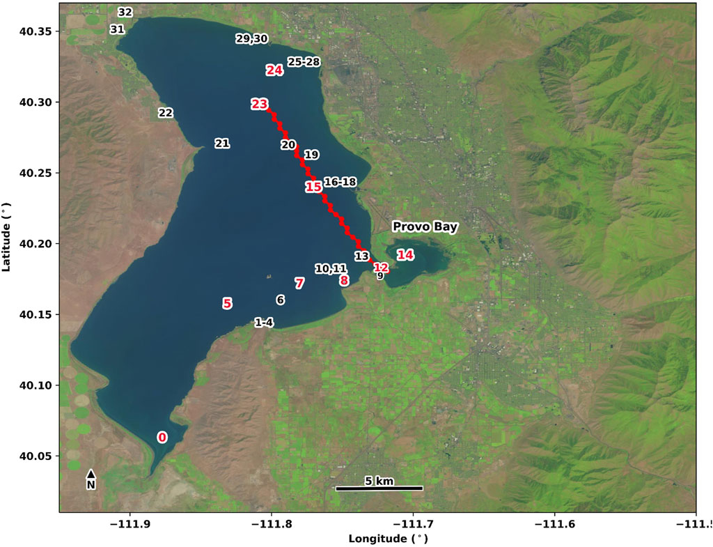
FIGURE 1. Utah Lake in Utah Valley, United States with in situ cell density sampling locations designed and visited by Utah DEQ. Select sampling locations (red labels) are displayed in Figures 6, 8. Satellite products from a stacked transect (red points) passing through stations 12, 15, 20, and 23 are shown in Hovmӧller diagrams (see Figure 7).

Widespread cyanoHABs on Utah Lake have been programmatically monitored by the Utah Department of Environmental Quality (Utah DEQ) and the Utah Department of Health (Utah DOH) since 2014 but have been a known issue since at least 1972 (Strong, 1974). Utah DEQ has used satellite imagery from a variety of sources as an internal screening tool to strategize sampling locations on Utah Lake and to communicate bloom extent and magnitude to local public health managers since 2016. These data have shown to be a valuable resource for monitoring cyanoHABs in Utah Lake; Stroming et al. (2020) found that early detection of a Utah Lake high magnitude cyanoHAB through satellite imagery saved roughly $370,000 in health care costs by reducing the public’s risk of exposure to cyanobacteria and cyanotoxins. For many years, cyanobacteria blooms on Utah Lake have started in spring and continued through winter, making the lake an ideal location for exploring new methods for mapping spatiotemporally cyanoHAB products from satellite observations.

3.2 Data assembly

3.2.1 Model development data

The in situ model development dataset (Figure 2) is nearly identical to the dataset used to train MDN-PC for imagery from the Hyperspectral Imager for the Coastal Ocean (HICO), covered in full within O’Shea et al. (2021). The main adaptation made to the MDN-PC training dataset for OLCI is that the remote sensing reflectance spectra (R_rs) were resampled with the relative spectral response functions of OLCI. The in situ training dataset spans a broad geographic range, including Lake Erie (N = 375), lakes of Indiana (N = 151), lakes of Spain (N = 125), Dutch lakes (N = 186), the Curonian Lagoon (N = 63), lakes of Italy (N = 20), and South African reservoirs (N = 10) (Matthews et al., 2020). The median Chla, PC, and PC:Chla ratios of the original dataset are 33.4, 14.5, and 0.48 respectively (Figure 2). Any PC or Chla in the range of 0–0.1 mg m⁻³ were set to 0.1 mg m⁻³, to keep the MDN from concentrating on discerning these nearly indistinguishable (from a water quality management perspective) concentrations. The dataset consists of a notably large proportion of low PC and low PC:Chla measurements (Figure 2), which are necessary for training the MDN for PC estimation from mixed phytoplankton blooms, where accessory pigments may impact the spectral signature. A low proportion of PC measurements from the in situ dataset are above 200 mg m⁻³, which may limit the ability of the MDN to learn how to most accurately predict the highest PC concentrations often associated with high-intensity blooms. Overall, the available dataset enables the MDN to train on PC across four orders of magnitude, with a particular focus on low concentrations typical of early bloom formation, spanning a wide geographic range.

FIGURE 2

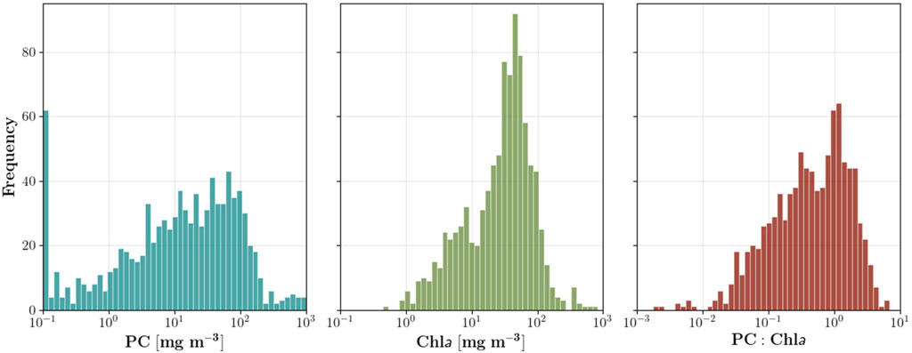
FIGURE 2. Log-scale histograms for in situ PC, Chla, and the PC to Chla ratio (PC:Chla) datasets (N = 930). These histograms are nearly identical to those used to develop the original HICO MDN (O’Shea et al., 2021). The median, mean, and standard deviation for Chla, PC, and the PC:Chla ratio are (33.4, 45.6, 59.5), (14.5, 49.9, 107.3), and (0.48, 0.83, 0.91) mg m⁻³, respectively.

3.2.2 Utah DEQ cyanobacteria in situ data

Utah DEQ has been routinely collecting in situ cyanobacteria cell density (cells mL⁻¹) data during the recreation season, which runs from mid-May through October, since 2017. The purpose of cell density data collection is to inform management decisions in the Utah DEQ and Utah DOH Harmful Algal Bloom Program, which utilizes cyanobacteria cell density thresholds for recommending health advisories to local health departments (UDEQ, 2020). During the recreation season, Utah DEQ monitoring teams sample Utah Lake either weekly or monthly, depending upon resources, and collect data at sites in the most frequented recreation spots along the shoreline, such as beaches and marinas, and in the open waters of the lake. While some sites are sampled consistently, Utah DEQ guidelines direct crews to sample ‘the most reasonable maximum’ part of an observed cyanoHAB, which represents the site of highest risk of exposure to recreators. This means cell density samples may be biased towards higher volumes and are not spatially comprehensive for each sampling event. Both a surface and water column (elbow depth, <1 m) composite sample can be collected, but not always both for each sampling site; often surface samples are prioritized if surface cyanobacteria scum is observed whereas composite samples are taken either concurrently with surface samples or singularly if no surface scum is observed. Taxonomic analysis and cell enumerations of all phytoplankton taxa are performed by PhycoTech, Inc. (St. Joseph, MI, United States) using a McClane Research Laboratories, Inc. (East Falmouth, MA, United States) Imaging FlowCytobot, a semi-automated imaging system, and reported in units of cells mL⁻¹. For this analysis, only cell concentrations of cyanobacteria taxa were used as a proxy measurement for in situ PC concentrations. Additionally, only data that were collected within ±4 h of OLCI and MSI overpass were used in this study. Utah DEQ also uses stationary, high-frequency (every 15 min) water-quality sondes on buoys in Utah Lake that collect both chlorophyll and a blue-green algae phycocyanin proxy measurements, but these data were not used in this study as sonde sensor calibration methods were inconsistent.

3.2.3 Satellite data processing

The OLCI and MSI imagery is processed to R_rs using the atmospheric correction for OLI ‘lite’ (ACOLITE, (Vanhellemont & Ruddick, 2021)) algorithm, which has proven to operate reasonably well for highly turbid and eutrophic inland waters (Pahlevan et al., 2021b), i.e., 20%–25% median uncertainties in the green and red bands. Two different versions of ACOLITE were used during processing, as the processing routine was updated while imagery was being processed. Both ACOLITE versions used in this manuscript were from prior to the updates provided in ACOLITE version V20221025, which fixed OLCI imagery being corrected for gas transmittance twice by ACOLITE and switched to applying the system vicarious calibration (SVC) gains from the European Organisation for the Exploitation of Meteorological Satellites (EUMETSAT) gains by default (as per the ACOLITE User’s Manual V20221025). The flag masks were empirically adjusted to return a higher proportion of pixels for the highly reflective waters of Utah Lake (Supplementary Appendix Figure SA1). The ‘L2w_mask’ threshold (applied at 1,600 and 1,020 nm for MSI and OLCI respectively) was set to 0.25 (unitless reflectance) and the ‘l2w_mask_high_toa_threshold’ applied to the TOA reflectance was set to 0.5 (unitless reflectance). The MSI target resolution was set to 60 m, to match the spatial resolution of the coarsest band (443 nm) used as input to MDN-Chl. Additionally, the ‘l2w_mask_smooth’ feature was turned off, to increase nearshore coverage. The number of valid aquatic pixels was further increased by empirically tuning the atmospheric flags to the specific aquatic signal of Utah Lake. Note that no radiometric spectra were available across Utah Lake for evaluating the quality of ACOLITE-derived R_rs products (see Supplementary Appendix A1 for sample R_rs).

3.3 Machine learning-derived PC estimation

Although other machine learning algorithms have been used for remote sensing of water quality (ex: Chen et al., 2021), for this study, we chose to use MDNs for predicting Chla and PC from satellite imagery. Prediction of Chla and PC from satellite imagery can be a complex task since these pigment values can vary due to a number of biotic and abiotic factors. Traditional machine learning models may struggle to deal with situations where the same reflectance value from remote sensing data corresponds to different pigment values under different conditions; known as the one-to-many problem (Bishop, 1994). Instead, an MDN can model the pigment value as a mixture of different probability distributions, each representing a different possible scenario. Then, when given a remote sensing reflectance value, the MDN can better account for variability and uncertainty in predicting pigment values, potentially leading to more accurate and robust predictions.

MDNs have been developed and proven for a variety of aquatic remote sensing product retrieval tasks from inland and coastal waters using multiple different sensors, including Chla retrieval from MSI, OLCI, and the Operational Land Imager (OLI) (Pahlevan et al., 2020; Smith et al., 2021), the retrieval of phytoplankton absorption (a_ph) from the Hyperspectral Imager for the Coastal Ocean (HICO) (Pahlevan et al., 2021a), particulate backscattering retrieval from six different satellite sensors (Balasubramanian et al., 2020), and PC retrieval from HICO and the PRecursore IperSpettrale della Missione Applicativa (PRISMA) (O’Shea et al., 2021). Clearly, MDNs are effective at retrieving a variety of different products for aquatic remote sensing tasks, even though the problem is non-unique and in situ training data is relatively limited.

For this research, two different MDNs were utilized, one MDN proven for Chla retrieval from MSI (Pahlevan et al., 2020) (hereafter MDN-Chl) and another MDN retrained for PC retrieval from OLCI. The Chla retrieval MDN trained for MSI was previously shown to achieve high accuracy Chla estimates, with a median absolute percentage error (MAPE) of 24% on the held-out in situ training dataset (Pahlevan et al., 2020). The MDN-PC for OLCI was trained using an identical architecture and nearly identical training set as the original PC retrieval MDN proven for HICO and PRISMA, but with the in situ spectra resampled to match OLCI (O’Shea et al., 2021). Another difference in the model development was the selected band ratios and line heights; the MDN-PC model leverages the 13 highest correlation band ratios in the 510–720 nm range (with a cutoff of 0.35) and the line-height centered at 673.75 nm (using the surrounding bands at 665 nm and 681.75 nm) as input features. The exact band ratios used were: [560, 510], [664, 510], [664, 619], [673, 664], [681, 510], [681, 664], [681, 673], [708, 510], [708, 560], [708, 619], [708, 664], [708, 673], and [708, 681]. The 510–720 nm range used as input for PC estimation was chosen to avoid the particularly high uncertainties in the blue bands that occur during atmospheric correction of the hyperspectral imagery it was originally trained for (Ibrahim et al., 2018); while the full range for MSI (443–783 nm) was used for Chla estimation (Pahlevan et al., 2022). Overall, both of these retrieval algorithms have been rigorously tested in prior research, and proven to provide improvements in Chla (MDN-Chl) and PC (MDN-PC) retrievals from optically complex inland waters. It should be noted that our previous research suggests that for estimating a single target variable like Chla (or PC), the choice of model architecture does not drastically boost the performance (Smith et al., 2021).

Although MDN-PC trained for HICO bands has been rigorously tested, in this work we further tested MDN-PC trained for OLCI-like R_rs (and its derivative indices) to demonstrate that the lower number of bands available on OLCI (and lack of 650 nm band) do not significantly limit algorithmic performance. MDN-PC trained for OLCI bands was validated on one-half of the in situ dataset, by first training an independently selected half of the dataset (∼465 samples) and then testing on the other half (see Figure 3). While this is an idealized performance assessment, since the samples originate from the same field campaigns and do not suffer from atmospheric correction uncertainties associated with satellite imagery; the 50/50 split still serves as useful method to determine if the available in situ dataset and spectral bands are sufficient to represent the target variable (PC) and to compare against alternative algorithms performance using the same approach (O’Shea et al., 2021; Werther et al., 2022). We gauged the performance of MDN-PC by reporting the median symmetric accuracy (ε), symmetric signed percentage bias (β), and slope (S) estimated via the Theil-Sen estimator (O’Shea et al., 2021), a set of metrics allowing for comparisons with previously developed models:

$\begin{array}{c}ϵ={100\times (10}^Y-1)\left[\%\right]whereY=Median\left|{\mathit{log}}_{10}\left(P{C}_s/{PC}_i\right))\right|\\ \left.\beta ={100\times sign\left(z\right)(10}^{\left|Z\right|}-1)\left[\%\right]whereZ=Median\left({\mathit{log}}_{10}(P{C}_s/{PC}_i\right)\right)\end{array}$

where $P{C}_s$ and ${PC}_i$ are satellite-derived and in situ measured PC, Median is the median operator, $ϵ$ represents the median symmetric accuracy, and $\beta$ is the symmetric signed percentage bias.

FIGURE 3

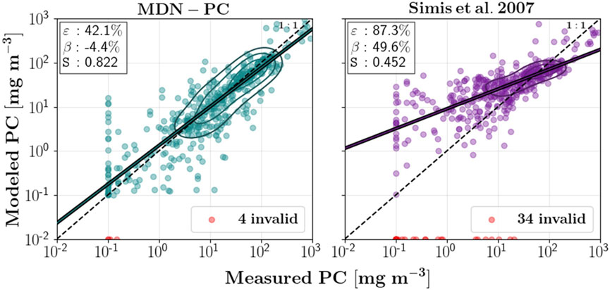
FIGURE 3. Modeled versus measured PC using one-half of the training set for training the MDN, and the other half for testing the MDN for OLCI on S3. Simis et al. (2007) estimates were performed using the standard coefficients. Invalid estimates (negative or non-finite for either algorithm or outside of 0.1–1,000 mg m-3, the range of the training data, for MDN-PC) are shown in red. Median symmetric uncertainty (ε), symmetric signed percentage bias (β), and slope (S) are displayed on the plot of each algorithm.

3.4 MDN performance analysis

A comprehensive assessment of MDN-based pigment estimates is essential not only to fully understand its strengths and weaknesses, but also to optimize its use in large-scale monitoring applications. To that end, multiple approaches including matchup assessments, time-series analyses, cross-validation, and risk-category evaluations were considered.

3.4.1 Matchup assessment

Despite the absence of in situ PC data in Utah Lake, we carried out a correlation analysis between our products (i.e., MDN-PC and MDN-Chl) and Utah Lake in situ cyanobacteria cell density data (Section 3.2.2.) to determine how well our predictions correlate with these in situ measurements. This analysis was similarly performed for CI-cyano products described below. Similar to Section 3.3, we reported median log-based metrics (ε, β) and slope to report model efficiency.

3.4.2 Cross-validation

To compare our OLCI-based MDN-PC maps to the widely used CI-cyano index, we used data processed through the CyAN framework (Schaeffer et al., 2015). CyAN provides daily CI-cyano products for the continental U.S. (CONUS) from different satellite sensors including MERIS (2002–2012), OLCI-A (2016-present), and OLCI-B (2018-present) at a 300 m spatial resolution. Daily CI maps for CONUS in 2018 were accessed directly through the Ocean Biology Processing Group data webpage for CyAN data (https://oceancolor.gsfc.nasa.gov/CYAN) (NASA Ocean Biology Processing Group, 2018) and further masked to Utah Lake’s spatial extent. For CyAN maps, CI-cyano is provided as an 8-bit raster with values ranging from 0–255 and flags for data below threshold detection limits, land, and no data. To focus on cyanobacteria biomass observations, we masked out all land and all no-data pixels. The 8-bit digital number (DN) data were converted to CI-cyano and cyanobacteria biomass estimates of cell density (cells mL⁻¹) using the equation provided by CyAN for conversion (CI-cyano = 10⁸ * 10^{(3.0/250*DN - 4.2)}) (NASA Ocean Biology Processing Group, 2018). It is worth noting that the MDNs have been shown to outperform several other state-of-the-art algorithms in previous research (O’Shea et al., 2021).

3.4.3 Spatiotemporal analysis

The 2018 OLCI and MSI images (May–October) processed via ACOLITE were reduced to MDN-PC and MDN-Chl time series to determine the suitability of our retrievals for cyanoHAB management applications (Figure 6). This year was chosen because near-weekly in situ cyanobacteria cell density data from Utah DEQ showed consistent, widespread cyanoHABs through the entire season, allowing us to evaluate spatiotemporal consistency of our maps first in comparison to in situ cell density data and second, against CI-cyano daily maps.

To determine how more spatiotemporally coherent daily maps of cyanobacteria biomass in Utah Lake could be created we examined how MDN-PC, MDN-Chl, and CI-cyano predicted bloom magnitude over time and space. The vastness of Utah Lake, coupled with the relatively short study period (185 days), presented a challenge to effectively capturing all spatiotemporal dynamics in the field sites during the recreation season. Hövmoller diagrams were used to visualize spatial and temporal variability of bloom magnitude along select transects and compare individual field sites over time through the use of a third dimension, bloom magnitude, represented as a color gradient (D’Ortenzio & Ribera d’Alcalà, 2009; Hovmöller, 1949). In this study the Hövmoller diagrams depicted a linear transect running NW to SW across the lake and intersecting at four individual sites (Figure 1).

Individual diagrams were created representing daily satellite observations for MDN-PC, CI-cyano, and a composite between MDN-PC and MDN-Chl. For same-day capture of OLCI-A and -B imagery, predicted PC values were averaged between the two sensors. To create the composite diagram, MDN-Chl data were used to fill in missing observations for MDN-PC. Composites were made by inserting MDN-Chl data only for days and locations that did not have data represented by MDN-PC. In cases where MDN-PC and MDN-Chl data were both available for a given location and time, MDN-PC was always chosen as the representative data point. Because each in situ site refers to a discrete geographic coordinate, differences in pixel size across the three algorithms did not present an issue.

3.4.4 Risk categories

To evaluate how our MDN-PC estimates compared against in situ data and CI-cyano for cyanoHAB decision-making applications over the course of a recreation season, we categorized each observation for all three data types into risk management categories. Here, we focused specifically on MDN-PC as the primary way to evaluate spatiotemporal cyanobacteria biomass across the entire lake’s sampling locations and omitted risk categorization of MDN-Chl, which is less specific to cyanobacteria and was used as a complementary data source in our multimission framework. Risk management categories are based on the WHO thresholds for a low, moderate, and high probability of adverse health effects from exposure to cyanobacteria in recreational waters (World Health Organization, 2003). The WHO classifies risk categories by both cyanobacteria cell density and Chla, but they can also be converted and applied to PC (Bastien et al., 2011; O’Shea et al., 2021) with “low-risk” defined as cell density <20,000 cells mL⁻¹ and PC values <20.0 mg m⁻³, “moderate-risk” cell densities of 20,000–100,000 cells mL⁻¹ and PC values 20–95 mg m⁻³, and “high-risk” cell densities >100,000 cells mL⁻¹ and PC values >95 mg m⁻³. Although Utah DEQ does not currently use this WHO risk management framework exactly, it has built its cyanoHAB advisory system around WHO thresholds for several years (UDEQ, 2020), as do many other states (USEPA, 2019). For both MDN-PC and CI-cyano, values of zero were included as low-risk because they represent a recoverable observation, even if they are below biomass detection thresholds. After risk management categorization, confusion matrices were created for both MDN-PC and CI-cyano where in situ data represent the observed/true value for a given day and site, and the satellite retrievals represent the predicted values. Same-day in situ and satellite-derived spatiotemporal pairs (i.e., coincident date and site matches) were used to evaluate categorical accuracy and error. Here, we define these as same-day in situ ‘matchups’. Note that the choice for matchups over broader, same-day data (Section 3.2.2.) was made to improve the statistical robustness of this risk assessment.

4 Results

4.1 MDN-PC: In situ performance analysis

MDN-PC for OLCI achieved a median symmetric uncertainty (ε) of 42.1/43.7%, a symmetric signed percentage bias (β) of -4.4/-2.6, and a slope (S) of 0.822/0.816 on a held-out half of the in situ training set (Supplementary Appendix Figure S3A,B Figure 3 not shown because of virtually identical performance). The uncertainty, bias, and slope generally agreed with the error metrics achieved by the original MDN-PC developed for HICO bands (O’Shea et al., 2021), despite the extreme reduction in bands available on OLCI. While the limited band availability makes the comparison to multiple models limited, the Simis et al. (2007) algorithm (using default coefficients) had substantially higher uncertainties, invalid estimates, and was biased high (particularly at low concentrations). It is worthwhile to note that O’Shea et al. (2021) showed that tuning the two coefficients for the Simis et al. (2007) algorithm to the training half of the dataset offered insignificant improvements in approximating PC. MDN-PC developed for OLCI bands continued to provide higher accuracy at lower concentrations (<10 mg m⁻³), with lower invalid estimates than multispectral algorithms, even though fewer bands were available relative to the original model. Overall, MDN-PC developed for OLCI matched the accuracy of the original MDN developed using HICO bands and outperformed alternative PC estimation models available for the limited number of bands (particularly at low PC).

4.2 MDN-PC comparison to in situ cell density

We used in situ cyanobacteria cell density to validate a) the MDN-PC and MDN-Chl products as proxies for cyanobacteria biomass and b) CI-cyano estimates of cell density (Figure 4). Of the three retrieved products, MDN-PC products (N = 38) and MDN-Chl products (N = 36) have the highest Pearson’s correlation coefficients (R, in log space), at nearly identical values of 0.72 and 0.74, respectively. Both MDN-PC and MDN-Chl were able to estimate products across the full dynamic range of available in situ cell densities (cell densities from <10³–10⁷ cells mL⁻¹), whereas CI-cyano cell density retrievals (N = 41, with 20 below threshold estimates) were sparse for waters with low in situ cell densities (e.g., <∼5*10⁴ cells mL⁻¹). At these lower ranges, CI-cyano begins estimating below threshold values (vertical pink lines, Figure 4), which correspond to predictions less than 10,000 cells mL⁻¹. These below threshold products predicted by CI-cyano were excluded from calculation of the correlation coefficient (R = 0.27). The below threshold estimates of CI-cyano often underestimated the in situ values, with 17 of the 20 below threshold estimates having associated in situ measurements above the ∼10,000 cells mL⁻¹ cutoff. Additionally, the CI-cyano response at higher concentrations is biased high. Overall, MDN-PC and MDN-Chl both had the best correlation to in situ cell density, and represented cell densities over the entire dynamic range within Utah Lake, which is a critical attribute for the detection of blooms at initiation and peak densities.

FIGURE 4

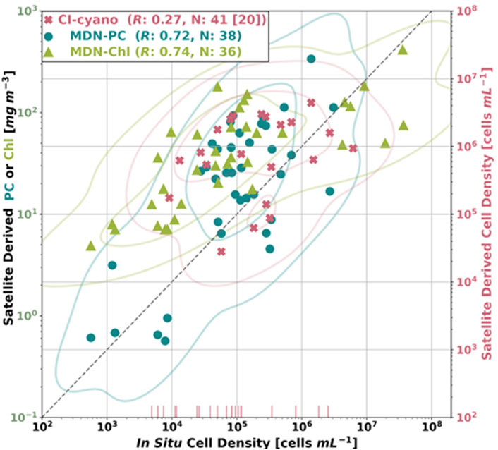
FIGURE 4. MDN-PC, MDN-Chl, and CyAN retrievals plotted against same-day (±4 h) in situ cell density measurements taken from thirty-three distinct locations within Utah Lake. CI-cyano satellite-derived cell densities beneath the CI-cyano sensing threshold (10,000 cells mL-1) are represented as vertical lines (the number of below threshold estimates is shown in brackets after the total number of CI-cyano estimates in the legend). The correlation coefficient (in log space) in the legend for CI-cyano does not include the below threshold values. A 1:1 line between In Situ Cell Density (x axis) and Satellite Derived Cell Density (right-hand y axis) is shown as a gray dashed line. The solid curves represent contour lines.

4.3 Spatiotemporal cyanoHAB dynamics

The full spatiotemporal variability of cyanoHABs as captured by MDN-produced maps in 2018 is illustrated in Figures 5, 6. The temporal coverage spanned from May 16, when both Sentinel-2 and -3 missions overpass Utah Lake, and extended to October 31 when the bloom monitoring season ended. High PC and Chla concentrations in the Provo Bay and southern shallow sections of the lake (Station 0) were detected early in the season. These local patterns significantly intensified and partially spread into open waters by early and/or mid-June. Blooms appeared to fluctuate in magnitude and extent in June and began to persist and expand in July with high-intensity periods throughout August and the first half of September. The blooms started to subside towards the end of September and dissipated at the end of October, although the overall lake-wide average PC appeared to remain higher than the values detected in mid-May.

FIGURE 5

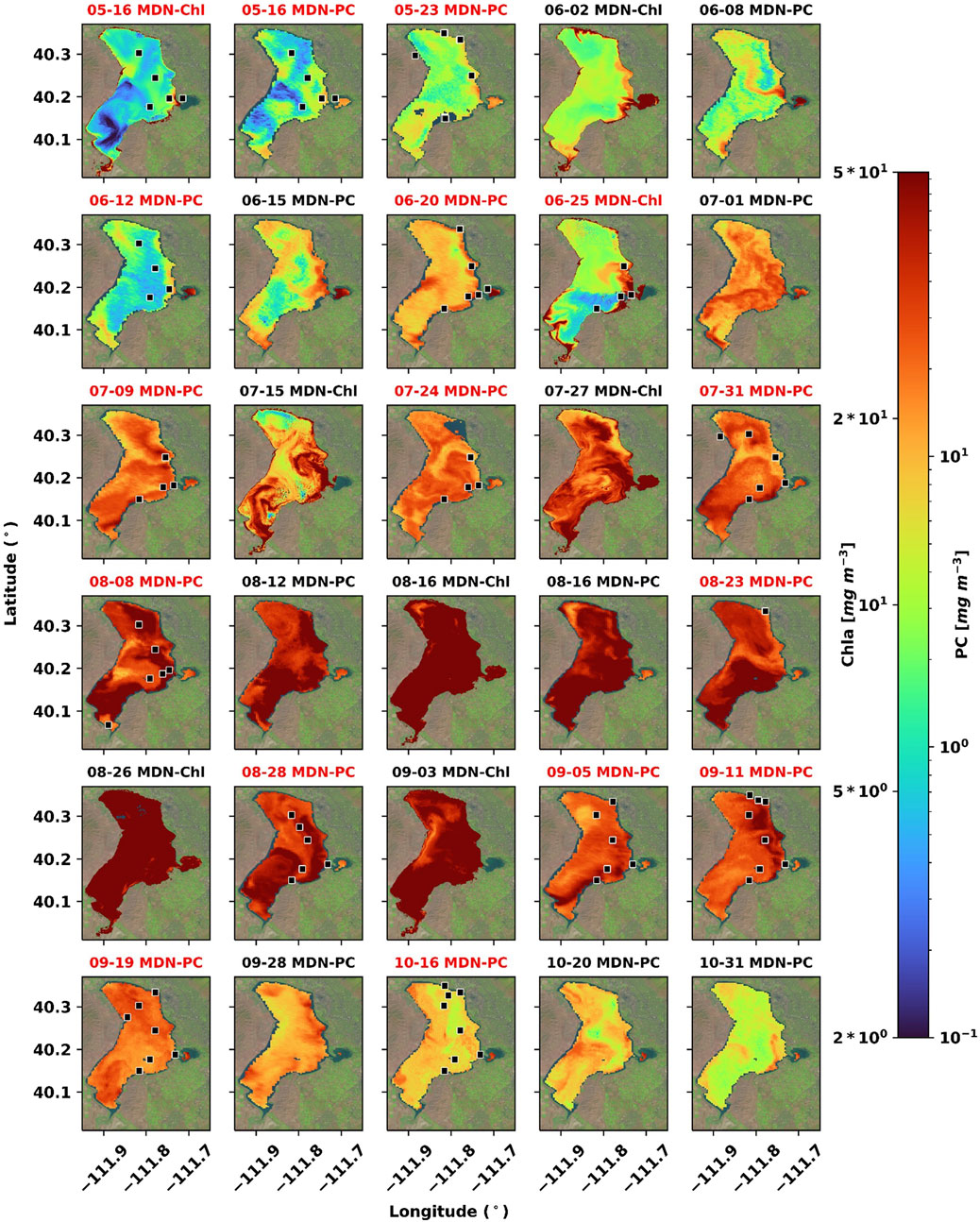
FIGURE 5. Maps of MDN-PC and MDN-Chl in Utah Lake for 2018. These maps do not represent the full temporal stack of available predictions for either model; dates were chosen to highlight the ability of MDN-PC and MDN-Chl to capture season-wide bloom dynamics. Dates that overlap with in situ sampling are labeled in red and sample stations for a given day are marked in black squares; squares are not to scale.

FIGURE 6

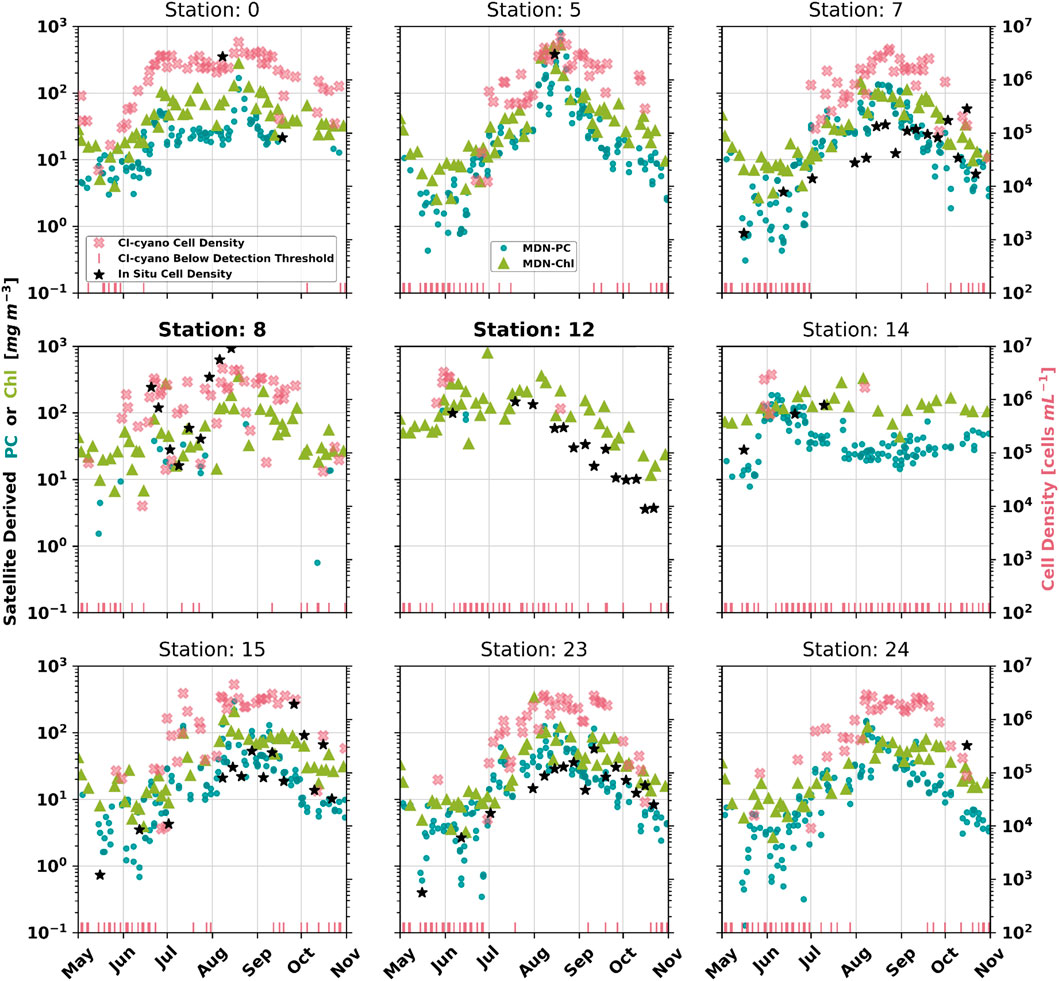
FIGURE 6. Time series of MDN-PC, MDN-Chl, and CyAN (cell-density) products derived from satellite imagery of select in situ cell density sampling sites across Utah Lake (Figure 1), as well as the corresponding in situ cell density matchups from those locations. The sampling locations are provided on a map of Utah Lake (Figure 1). The full set of matchups are also available in the appendix (Supplementary Appendix Figure SA2, A3). CI-cyano satellite-derived cell densities beneath the CI-cyano sensing threshold were set to 100 for plotting convenience.

The ability of each of the three algorithms (MDN-PC, MDN-Chl, and CI-cyano) to represent relative changes and key timings within bloom formation can further be visually assessed via time series plots (Figure 6) at specific sampling locations (Figure 1). For this analysis, nine of the thirty-three available in situ cell density sampling locations within Utah Lake, for the year 2018, were chosen for their 1) spatial coverage, 2) in situ measurement abundance and temporal coverage, and 3) spatial resolution requirement (e.g., nearshore Stations 8 and 12, bolded in Figure 6). All three algorithms responded to changes in situ measured cell densities above ∼5 × 10⁴ cells mL⁻¹. Additionally, all three algorithms captured peak cell density timings well (Figure 5, Stations 5, 7, 15, and 23). The first major difference between the three algorithms occurred with product retrievals in waters with particularly low cyanobacteria cell densities (∼10²–10⁴ cells mL⁻¹), (Figure 6, Stations 7, 15, and 23). Notably, MDN-PC and MDN-Chl retrievals were less sparse near to days with in situ cyanobacteria cell densities of ∼10²–10⁴ cells mL⁻¹ relative to CI-cyano (Figure 6, Stations 7, 15, and 23). MDN-PC retrievals responded to low cell densities, in addition to representing bloom peaks (∼10⁶–10⁸ cells mL⁻¹), covering nearly five orders of magnitude, and thereby capturing the entire bloom life cycle (Figure 6, Stations 7, 15, and 23). The second major difference between the three algorithms was the ability of MDN-Chl to offer the best remote observation of cyanobacteria cell density in nearshore regions (Figure 6, Stations 8 and 12, bolded), as it relies on MSI imagery, which has a substantially higher spatial resolution (60 m per our choice of grid cell size, Section 3.2.3) compared to OLCI’s nominal resolution (300 m).

Across the transect that intersects with four of the Utah Lake in situ stations (Figures 1, 7), MDN-PC, MDN-Chl, and CI-cyano showed distinct spatial and temporal patterns, both of which have reaching consequences for recreational risk management. To further elucidate the spatiotemporal relationships related to bloom magnitude between discrete in situ data points and satellite-derived predictions, in situ data were inserted into each diagram (Figure 7).

FIGURE 7

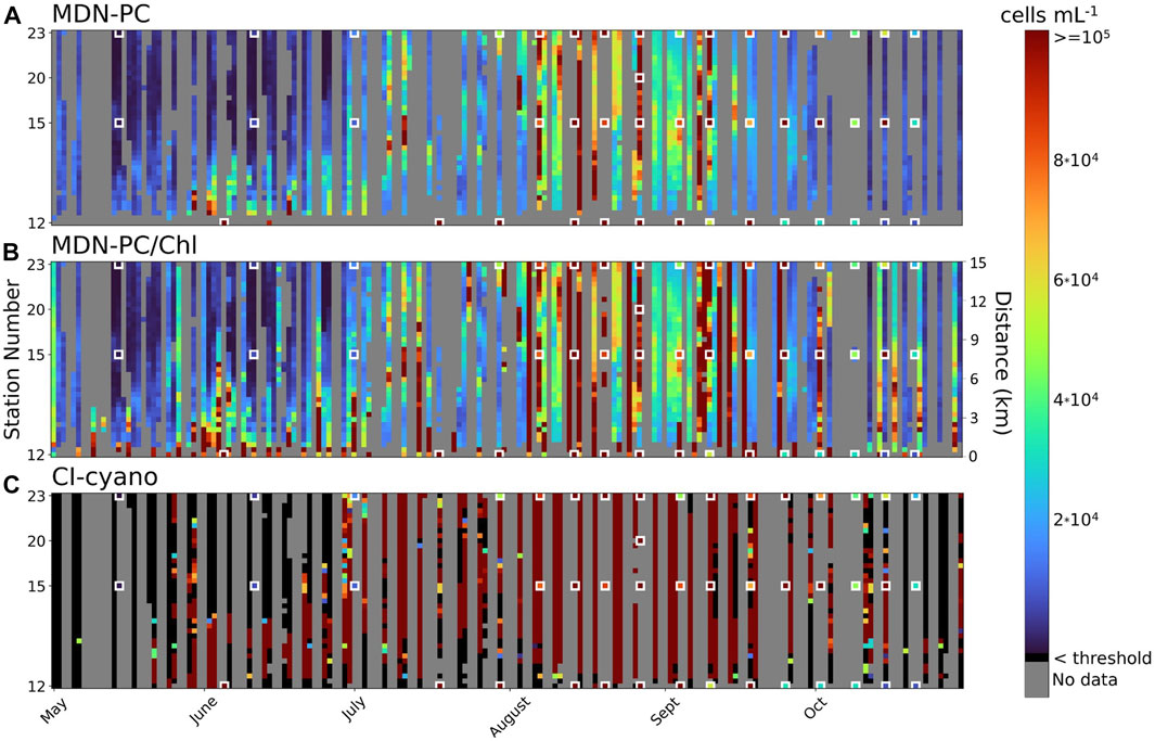
FIGURE 7. Hövmoller plots of MDN-PC (A), MDN-PC and MDN-Chl (Methods, Spatiotemporal Analysis) (B), and CI-cyano (C) predictions of bloom biomass from May through October 2018 for a 39-pixel transect that runs NW (pixel position 0) to SE (pixel position 38) through sites 12, 15, 20, 23 (see Figure 1). Each cell represents bloom magnitude predictions. In-situ measurements are overlaid on each plot and outlined in red. Colorbar gradient refers to bloom magnitude in cells mL-1 but each algorithm is mapped to its corresponding unit (mg-3 for MDN-PC and µg for MDN-Chl).

From May through October (left to right), the Hövmoller plots showed a distinct bloom pattern seen through all three algorithms. The bloom begins to form in the southeast portion of the transect (near Station 12) and advances northwest (towards the top) through the transect before spreading throughout the entire transect in August, increasing in magnitude over time. After peaking in both magnitude and extent in September, the bloom reduces in magnitude and only the southeast portions are still affected by the end of October. While all three algorithms show a similar spatiotemporal cyanoHAB dynamic for this transect in 2018, the spatiotemporal aspects of the bloom magnitude differentiate the algorithms from each other.

MDN-PC first detected the bloom at low magnitude in late May, with only a few observations predicted within the high-magnitude range (∼80,000 to >100,000 cells mL⁻¹). From August through September, MDN-PC predicted a patchy and ephemeral high magnitude bloom for several days, with bloom magnitudes between PC values of ∼38–75 mg m⁻³ (equivalent to ∼40,000–80,000 cells mL⁻¹). After mid-September, the MDN-PC indicated the bloom was reducing to lower-magnitude cell concentrations (equivalent to ∼10,000–20,000 cells mL⁻¹) through October. MDN-PC matched up with spatiotemporally coincident and closely adjacent in situ data for most of the recreation season and accurately predicted low, moderate, and high magnitude bloom concentrations. However, in September, MDN-PC underestimated several high-magnitude bloom events at the labeled in situ site data markers.

Adding MDN-Chl data (Figure 7B) to missing MDN-PC observations improved the spatiotemporal coherence of MDN-PC’s ability to track the cyanobacteria bloom dynamics. One of the biggest improvements came from adding data to a point on the transect that had no data with MDN-PC alone. For example, Station 12 sits in the spatial context of an inlet that is ∼225 m wide, a feature that OLCI is often unable to resolve because of spatial resolution constraints. With the addition of MSI data and MDN-Chl, bloom dynamics can be tracked at this location. MDN-Chl predicted a high-magnitude bloom in the southeast portion of the transect that was persistent from May through mid-September, matching with spatiotemporally adjacent and coincident in situ data. In addition to spatial augmentation, MDN-Chl also increased the temporal density of MDN-PC observations, filling in missing data across the recreation season.

While CI-cyano exhibits the same broad, spatiotemporal bloom dynamics over the transect and course of the recreation season, it differs significantly in its capture of spatiotemporal variability of bloom magnitude. From May through October, CI-cyano predicts that the majority of the bloom is high magnitude (≥100,000 cells mL⁻¹) as it moves through the transect and months. This does not match spatiotemporally adjacent and coincident in situ data, which show more spatial and temporal variability in bloom magnitude across the season and across the transect. Compared to MDN-PC, CI-cyano also does not capture low-risk bloom magnitude (<20,000 cells mL⁻¹) with the same precision and predicts the majority of the low-magnitude bloom areas as below detection threshold, whereas MDN-PC and MDN-Chl both provided absolute values of bloom magnitude through a range of PC and Chla.

The number of individual spatiotemporal bloom magnitude predictions from MDN-PC and CI-cyano were similar, with MDN-PC performing slightly better. Of the possible spatiotemporal data points across the 39-pixel transect and 185 days, MDN-PC predicted bloom magnitude 37% of the time and CI-cyano 36% of the time (including below biomass threshold observations). When below threshold observations were removed from CI-cyano, the percentage of total possible spatiotemporal observations with an absolute value prediction of bloom biomass was reduced to 16%. When MDN-Chl was added to MDN-PC, the number of MDN predictions increased by ∼38%, predicting bloom magnitude 51% of the time, significantly augmenting the spatiotemporal coherence of monitoring bloom dynamics. MDN-PC also surpassed CI-cyano in the number of days with any observations, predicting bloom magnitude for at least one portion of the transect for 48% of the recreation season, compared to CI-cyano at 38%. When MDN-Chl was added to fill missing data to MDN-PC, this percentage rose to 64% of the recreation season that had at least one observation.

4.4 Risk management categories

MDN-PC and MDN-Chl were better at representing the three risk categories (low/moderate/high) defined by in situ matchups (Section 3.4.4.) from nearby dates than CI-cyano data (Figure 8). In particular, MDN-PC and MDN-Chl performed better at predicting low and moderate risk categories, while CI-cyano typically overestimated moderate risk categories and did not produce products over low-risk categories (Figure 8, Stations 7, 15, and 23). While MDN-Chl captured risk categories quite well at Station 12, which requires a higher spatial resolution than OLCI provides, MDN-Chl underestimated the high-risk categories at Station 8. While the categorization is imperfect, MDN-Chl did capture the general bloom decrease followed by a bloom increase that occurred at the beginning of July near Station 8 (Figures 5, 6, 8). While MDN-PC seemed to best represent the low and moderate risk categories, CI-cyano best captured the high-risk categories. Overall, while MDN-PC did the best job representing all three risk categories, it is important to note that these risk categories were chosen based on WHO levels, which may not be perfectly applicable to each lake, and likely require region-specific tuning.

FIGURE 8

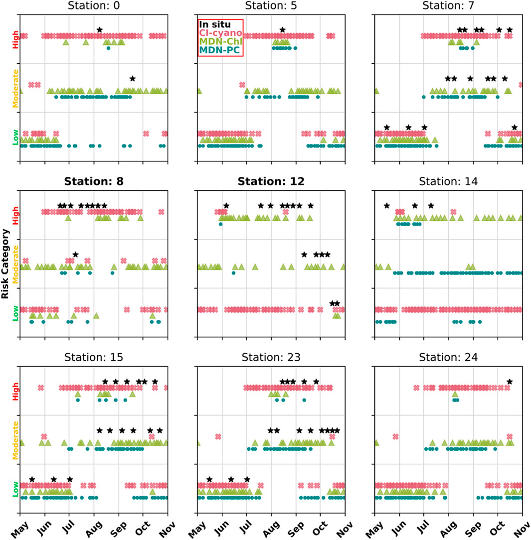
FIGURE 8. Risk categorized time series of MDN-PC, MDN-Chl, and CyAN products derived from satellite imagery for select sampling sites from Utah Lake (Figure 1), with in situ cell density matchups available. Risk categories were set using predefined thresholds, adapted from WHO recommendations (World Health Organization, 2003). For categorized time series of all lake sites please see Supplementary Appendix Figure SA2, A3.

In situ data, although limited in space and time, can also be used as a baseline for comparing algorithm performance from a risk-management perspective. This can be conducted by leveraging confusion matrices (Congalton & Green, 1999) and assessing corresponding accuracy metrics for each algorithm (Table 1). Confusion matrices of in situ risk categorization matchups show that MDN-PC performed exceptionally well in predicting low-risk in situ values 100% of the time with a false negative rate of 0% (Figure 9A; Table 1). CI-cyano performed fairly well with low-risk in situ measurement matchups with a 28% false negative rate. However, all of the false negatives came from misclassifying low-risk in situ matchups as high-risk, which is the largest categorical contrast possible (Figure 9B; Table 1). With a false negative rate of 93%, CI-cyano performed worse than MDN-PC with moderate-risk in situ matchups and misclassified moderate-risk in situ measurements as low-risk the majority of the time. CI-cyano did, however, outperform MDN-PC in high-risk in situ measurement matchup classification, correctly identifying high-risk in situ matchups 55% of the time. However, of the remaining false negatives, the majority came from misclassifying high-risk in situ matchups as low-risk, which is, again, the largest categorical contrast within the risk categorization schema. MDN-PC had a 79% false negative rate for high-risk in situ matchups but the majority of the misclassified matchups were predicted as moderate-risk.

TABLE 1

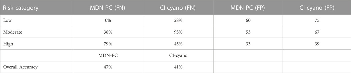
TABLE 1. False-negative (FN) and false-positive (FP) error rates for MDN-PC and CI-cyano and overall accuracy (number of correct predictions out of all total predictions).

FIGURE 9

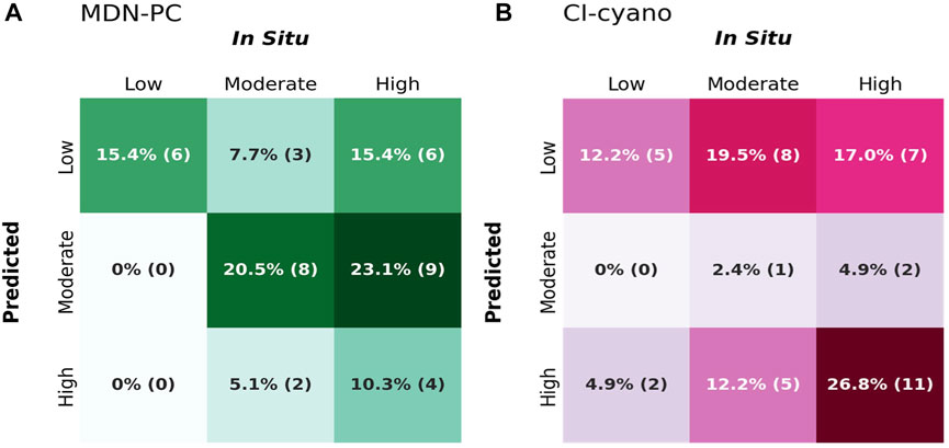
FIGURE 9. Confusion matrices for MDN-PC (A) and CI-cyano (B). Observed columns refer to risk management categories for in situ data and predicted rows refer to risk management categories for satellite-derived observations. For the total number of spatiotemporal matchups, N = 38 for MDN-PC and N = 41 for CI-cyano. Annotations refer to the percentage of total observations with the number of observations per cell in parentheses. The color gradient in the matrices represents these proportions, ranging from light to dark. Lighter shades correspond to lower proportions (0%), indicating fewer observations falling within these cells, while darker shades correspond to higher proportions (100%), indicating a larger number of observations. Correctly predicted cells in this context are darkly shaded diagonal cells, indicating high prediction accuracy by representing a high proportion of total observations. Incorrectly predicted cells are off-diagonal cells that are darker, as these represent more frequent misclassifications.

MDN-PC moderately overestimated the number of in situ matchups predicted to low-risk pixels with a false positive rate of 60% and classified high-risk in situ matchups as low-risk 44% of the time, representing a wide contrast in risk categorization. Similarly, CI-cyano had a 75% false-positive rate for predicted low-risk pixels. For both MDN-PC and CI-cyano, pixels predicted to be moderate-risk were almost identically split between being true positives for moderate-risk in situ matchups and false positives predictions of high-risk in situ measurements but never low-risk in situ matchups. However, MDN-PC predicted almost six times more moderate-risk pixel matchups with in situ measurements compared to CI-cyano. MDN-PC also outperformed CI-cyano in predicting high-risk pixels compared to in situ measurements and, unlike CI-cyano, MDN-PC never misclassified low-risk in situ matchups as high risk, unlike CI-cyano. Further, CI-cyano had nearly three times more high-risk predicted pixels than MDN-PC.

Broadly, both algorithms had bimodality in their spatiotemporal matchup risk-category prediction totals but with different risk-categories dominating predictions. Out of all predictions, MDN-PC classified 38% of the matchups as low-risk, 44% as moderate-risk and only 15% as high-risk. CI-cyano classified 49% of matchups as low-risk, 44% as high-risk, and only 7% as moderate-risk. Each algorithm had a gap in one category, but for different categories, which has different implications for risk management applications. Despite both algorithms having high true-positive and true-negative accuracies in one risk category but low in others, MDN-PC outperformed CI-cyano with an overall accuracy of 47% compared to 41% (Table 1). The overall accuracy does not capture the variability of risk-category prediction within the two algorithms in the same precision that examining individual true-positive and true-negative accuracies achieves. Further, there are limitations to this accuracy assessment because both algorithms had less than 40 individual in situ matchups over the entire recreation season; with a low number of data points to evaluate, each individual matchup can have a large effect on accuracy evaluation.

5 Discussion

In this study, we improved upon CyAN’s CI-cyano algorithm through building on a recently developed machine-learning technique (O’Shea et al., 2021) and supplemented OLCI-based PC maps with MSI-derived Chla products for enhanced spatial resolution along important shoreline areas with MDN-Chl (Pahlevan et al., 2020).

5.1 Mapping cyanoHABs using MDN-PC and MDN-Chl on satellite imagery

Moving towards a model that is independently tested and evaluated in time and space is imperative towards a widely-applied cyanoHAB mapping technique that can represent the bloom life cycle in the absence of in situ, laboratory-derived, PC, or Chla training data. Here we show that both satellite-derived Chla and PC can serve as a proxy for in situ cyanobacteria cell density over the entire life cycle of a bloom in Utah Lake, a region outside of the training set. Both PC and Chla enable a strong representation of the life cycle of a typical bloom, as seen in the same-day matchups (Figure 7), by quantifying a change in cell density of ∼4 orders of magnitude (∼10³–10⁷ cell mL⁻¹). The ability of both proxies to represent the full bloom life cycle in a new region is further supported via time series of a bloom with in situ samples at site-specific locations throughout the lake (Figures 5, 6). The capabilities of both provide higher fidelity, particularly at bloom onset, relative to state-of-the-art algorithms (e.g., CI-cyano, Figures 5, 7).

A combination of the MDN-PC and MDN-Chl can be used to increase the spatial and temporal coverage of cyanoHABs, by keeping in mind the limitations of each proxy (Figures 6, 9). Spatially, the main advantage of using both MDN-PC (on OLCI imagery) and MDN-Chl (on MSI imagery), is to determine the specificity of MDN-PC for cyanobacteria in open-water areas, and the finer spatial resolution available via MDN-Chl products for nearshore coastal regions. Temporally, MDN-Chl (MSI) can fill in for missed days in the MDN-PC (OLCI) dataset. In same-day overlaps between MSI and OLCI (ex: Figure 5 dates 5–16 and 8–16), there are distinct (and expected) observed differences in spatiotemporal bloom magnitude across the lake between MDN-Chl and MDN-PC. It is likely these differences exist from differences in spectral resolution and band availability between MSI and OLCI, and the possibility of detecting all photosynthetic biomass, including eukaryotic species, (seen through MDN-Chl) compared to just cyanobacteria (distinguished in MDN-PC). Looking closer, the differences between the two algorithms (Figures 4, 6) suggest that MDN-Chl overestimates early bloom formation, and underestimates peak bloom intensity, so while both individually represent the full bloom life cycle, the absolute differences in using the two algorithms for management decisions based on risk assessment still must be explored.

5.2 Management decision implications

Even though the US EPA has only issued guidance for some cyanotoxins as they relate to recreational exposure, for Utah Lake, Utah DEQ, and many other recreational cyanoHAB monitoring programs across the United States, risk management decision making goes beyond the measurement of cyanotoxins by necessity and complexity of stakeholder concerns (USEPA, 2019). With a consistent cyanotoxin sampling routine, Utah DEQ still takes other factors into account before recommending health advisories to local health departments (UDEQ, 2020). Current EPA guidelines specifically omit metrics of bloom biomass magnitude, bloom frequency, and bloom extent. However, it is these metrics that are among the most important that satellite imagery cyanoHAB monitoring frameworks can provide to augment recreational resource management.

5.2.1 Bloom magnitude

Bloom magnitude can be characterized in both the spatial and temporal domains and quantified by measures of cyanobacteria biomass. Here, we discuss bloom magnitude not as an absolute measure of peak bloom biomass for a given time period (Mishra et al., 2019), but rather as the representation of the biomass range that can be seen through different spatial and temporal scales. We found that both MDN-PC and MDN-Chl were able to represent both seasonal and intraseasonal temporal bloom magnitude patterns seen through the baseline of in situ bloom biomass data. Time series of individual sites (Figures 5–7) along with Hövmoller plots across in situ transects (Figure 7A) show that MDN-PC has the same pattern of low-risk bloom biomass values dominating the shoulder weeks of the recreation season and high-risk bloom values peaking August through September. This also fits with widely known dynamics of cyanoHAB phenology over a given year; as solar radiation (the number of clear, sunny days), hours of sunlight, and water temperatures all increase towards mid to late summer, cyanobacteria can outcompete other photosynthetic organisms and bloom in relative abundance, creating the highest public health risk under these conditions (Zhang et al., 2012; Coffey et al., 2019).

Knowing when and where the areas of high-risk, high-magnitude cyanobacteria biomass occur is imperative for making informed decisions about cyanoHAB advisories in Utah Lake and elsewhere. If satellite-derived maps of cyanobacteria biomass consistently overestimate cell density and bloom magnitude, managers will not be able to depend on this resource to make decisions. This characteristic of cyanoHAB detection is where MDN-PC shows great promise; through a more balanced and coherent spatiotemporal distribution of risk management categories, managers do not have to worry about overestimating risk and may be able to use the maps more effectively in risk management decision making. Compared to CI-cyano, MDN-PC best shows the full dynamic range of the blooms when spatial resolution is not a limiting factor, as confirmed by the in situ cell densities, but MDN-Chl well represents blooms in nearshore regions that cannot be captured by OLCI (Figures 4–7).

While MDN-PC has great potential to be incorporated into established cyanoHAB recreational water quality programs to monitor bloom magnitude, there are also limitations. Although MDN-PC is more reliable in mapping cyanoHAB risk, there is the contrasting issue of potential underestimation. While CI-cyano is biased towards predicting high-risk, high-magnitude predictions, MDN-PC is feasibly biased towards low-risk, low-magnitude predictions (Figure 9A). Because the Utah DEQ in situ sampling strategy is a mix of both routine and opportunistic data collection, it is difficult to obtain a true picture of the real cyanoHAB risk management category and bloom magnitude spatiotemporal distribution throughout the entire recreation season and the entire lake. In situ data will be inherently biased towards the ‘worst case scenario’ sampling that Utah DEQ employs, wherein the densest part of a cyanoHAB is typically sampled. This means for many days and/or samples, in situ data will reflect high risk cell concentrations when, in reality, there may be a more balanced mix of low risk and moderate risk areas across the entire lake that are not sampled because of resource limitations.

There is evidence to suggest that MDN-PC and MDN-Chl maps may elucidate new patterns of bloom magnitude (Figure 7A,B) and bring to light many more areas of low- and moderate-risk bloom magnitude compared to CI-cyano. As seen through the Hövmoller transect (Figure 7A), MDN-PC has more predictions of estimated PC (i.e., any estimation of bloom magnitude) than CI-cyano. More importantly, MDN-PC does significantly better in predicting actual values of cyanobacteria biomass at low and moderate-magnitudes compared to CI-cyano, which is unable to capture the same variability and precision at those levels and, instead, classifies them as being below detection threshold. The addition of MDN-Chl also allows more absolute values of biomass to be mapped in nearshore areas (Figure 7B) and fill spatiotemporal gaps otherwise missed by OLCI imagery due to spatial limitations. It could be that MDN-PC simply detects lower magnitude bloom biomass in a way that CI-cyano and in situ sampling do not and, therefore, has many more predictions in this class. While areas of low-risk biomass detection may not present immediate concern from public health authorities, they do represent areas of notice as low-risk can quickly turn to moderate- or high-risk with the right environmental conditions (e.g., elevated air temperature, wind patterns (Wynne et al., 2010)). Understanding where low magnitude blooms occur can help managers prepare for developing blooms and make informed decisions. Similarly, with frequent mapping, observations of spatiotemporal patterns of low- or moderate-risk areas allow managers to see bloom trajectories in space and magnitude which would allow the use of MDN-PC as a lake-wide cyanoHAB tracking tool, opposed to only mapping areas that have already reached high-risk. More in situ matchups, specifically PC sample collection, are needed to explore the potential for underestimation bias further and to understand what may be closer to ‘true’ spatiotemporal bloom magnitude over the recreation season.

5.2.2 Bloom frequency

Our study did not seek to answer specific questions about how frequently cyanobacteria blooms occur over short- and long-term temporal scales in Utah Lake but, rather, we sought to identify if MDN-PC and MDN-Chl were potential sources to help answer these questions in the future.

In comparison to CI-cyano, MDN-PC had an additional cumulative 18 extra days of any bloom biomass predictions in the Hovmöller diagrams, increasing monitoring of bloom frequency by more than two cumulative weeks (Figure 7A,C). Any added days of bloom magnitude predictions allows managers to make more immediate, accurate, and precise risk-management decisions regarding public health and resource management. In addition to OLCI-based algorithmic improvements with MDN-PC, adding MDN-Chl from MSI data also augments bloom detection frequency at a different, finer spatial scale (Figure 7B). By supplementing MDN-Chl predictions into the MDN-PC Hovmöller transect, an additional 30 extra days of bloom magnitude predictions occurred compared to MDN-PC alone and an extra 48 days compared to CI-cyano. With OLCI-based cyanoHAB biomass indicators, aquatic and public health managers’ ability to access near-shore satellite observations is dependent upon algorithmic parameters around detection within >300 m of land. While MDN-Chl may not offer the same precision in bloom biomass that cyanobacteria-exclusive PC or CI-cyano do, it still increases the frequency of cyanoHAB detection in important recreational areas such as beaches and marinas and could be used as a supplemental monitoring tool for open-water areas if managers need to understand bloom frequency for timely risk management decisions (Figures 4–6, 9). For example, for some sites, the use of MDN-Chl improves the frequency of satellite-based cyanoHAB observations from no observations to at least weekly, if not more frequently (Figures 5, 6, 9B).

5.2.3 Bloom occurrence and extent

Regarding temporal and/or spatial scale, there is no standardized definition of a cyanoHAB and interpretations of spatiotemporal cyanoHAB risk vary based on application. For example, a cyanoHAB can be defined relative to its spatial extent; examples include a specific two-dimensional size that biomass must reach for it to be considered a cyanoHAB or a certain percentage of the waterbody area covered by cyanobacteria biomass before management action is taken (Hu et al., 2010; Davis et al., 2019). Similarly, the temporal occurrence pattern of a cyanobacteria biomass can determine how a cyanoHAB is characterized; metrics of cyanobacteria biomass persistence, on any temporal scale, can inform thresholds of when biomass becomes a bloom (Coffer et al., 2020).

In addition to creating additional temporal coverage of cyanobacteria biomass compared to CI-cyano (Figures 6, 7), MDN-PC bloom magnitude predictions also considerably increased spatial coverage and capture of bloom biomass predictions over our study period. Although MDN-PC and CI-cyano had similar counts of total predictions (N = 2,667 and 2,543, respectively) within the Hovmöller diagrams (Figures 7A,C), those counts include predictions below biomass detection for CI-cyano, giving managers no insight into whether there is no cyanobacteria biomass at all or there is a low-magnitude bloom. By removing below detection threshold predictions, the CI-cyano biomass prediction count drops by more than 50% and becomes 57% lower than MDN-PC’s total predictions of biomass values. Spatial coverage of bloom biomass predictions is critical to cyanoHAB recreational health monitoring programs. For example, in the Utah DEQ and Utah DOH cyanoHAB monitoring program, state and local managers have the option to issue recreational advisories on a site-specific basis, as opposed to only issuing advisories for an entire waterbody. This, in practice, means that portions of the waterbody could be closed for recreational use while other areas remain open. For Utah Lake, spatial segmentation of recreational advisories has occurred every year since the cyanoHAB program inception (UDEQ, 2020). The decision to not issue a lake-wide advisory as soon as a cyanoHAB has been detected in one portion of the lake means managers must have a precise and accurate representation of bloom location, regardless of magnitude, on a frequent, if not daily, basis in order to track public health risks in real-time. If monitoring personnel are not able to visit the lake more than once a week or once a month (e.g., restrictions due to the COVID-19 pandemic), frequent satellite imagery becomes imperative and spatiotemporal gaps in daily maps could also lead to gaps in human health and environmental resource protection. With the distinct increase in spatial extent compared to CI-cyano data, MDN-PC and MDN-Chl can help managers make more informed, accelerated, and precise decisions about cyanoHABs.

Timing is also important to consider when discussing the increase in cyanoHAB observation occurrences that MDN-PC provides. MDN-PC added the most above biomass detection threshold spatial extent compared to CI-cyano in the early summer and fall (Figures 7A,C). This result is important because aquatic resource and public health managers do not just need reliable spatial coverage of cyanoHABs during intense bloom events that may occur in the mid to late summer weeks. Utah Lake can potentially be utilized for recreation and irrigation as soon as ice melts in the spring and up until ice forms in the fall or winter, so having a comprehensive picture of cyanoHAB spatial extent for as many days of the year as possible is imperative for keeping the community safe. Additionally, there is growing concern about the transport of cyanotoxins to crops and agricultural soils through the use of contaminated irrigation waters (Corbel et al., 2014), thus monitoring for the presence of cyanobacteria, and co-occurring cyanotoxins, should occur during all stages of crops’ growing cycles (May - September (Jones et al., 2020)). Although MDN-PC predicts majority ‘low risk’ pixels during the shoulder months, even low-risk cyanobacteria biomass has the potential to cause health issues (Pilotto et al., 1997) and is important to track.

As with cyanoHAB frequency, the addition of MDN-Chl maps has the potential to take satellite-based cyanoHAB observational occurrence from zero to extensive in some shoreline sites (Figures 4–6, 9). Even in some shoreline areas where both CI-cyano and MDN-PC may be able to reach, MDN-Chl improves upon spatial extent precision, which may be important for public health managers in determining health advisory locations. For example, Utah DEQ, Utah DOH, and the Utah County Public Health Department separate Lincoln Beach and Lincoln Marina as different locations for health advisories. These two sites are only ∼75 m from each other, making a 300-m pixel too coarse to distinguish between the two locations. However, with MDN-Chl, this spatial resolution is no longer a limiting factor in site-specific cyanoHAB occurrence precision.

5.2.4 Towards a spatiotemporally coherent cyanoHAB monitoring tool

Both short- and long-term trends of cyanoHAB metrics are essential to keeping public health and aquatic ecosystems safe. In the short term, the US EPA recommends that during the recreation season, measures and thresholds of cyanoHAB magnitude should not be exceeded on any single day in order to be protective of recreational activities and that when recreational advisories are issued, prompt information should be given to anyone who may consider water-based activities, such as swimming (USEPA, 2019). Daily in situ monitoring of all recreational areas is an enormous task that is likely unfeasible for most cyanoHAB programs and we showed that the satellite-based CI-cyano index may miss large swaths of bloom biomass predictions below detection threshold and tends to overestimate magnitude when cyanobacteria biomass is detected (e.g. Figures 6, 8, 9). Our methods present a new and more coherent way to ensure spatiotemporal metrics of cyanoHAB blooms are identified on a frequent basis during the recreation season compared to previous frameworks. First, MDN-PC and MDN-Chl maps combined produced substantially more frequent observations and cyanobacteria biomass predictions across Utah Lake compared to both in situ and CI-cyano, which would allow for timely and frequent communication about cyanoHAB bloom location. Second, MDN-PC and MDN-Chl showed a marked increase in cyanobacteria biomass spatial extent compared to the other methods and did so with a more comprehensive spatiotemporal distribution of bloom magnitude. It is not just areas of visible cyanobacteria scum that pose a risk to recreators and detecting areas of low-risk or low PC values hold value in risk communication of cyanoHABs. The absence of identification of these areas may lead to an underrepresentation of lake-wide or site-specific risk. Direct ingestion of algal scum or cyanotoxins is also not the only pathway towards inflammatory illness from cyanoHABs, exposure to any cyanobacteria cells (Pilotto et al., 1997) or aerosolized toxins (Plaas & Paerl, 2021) also presents a risk to public health. CI-cyano performs well during times of high magnitude and high-risk blooms but MDN-PC (supplemented by MDN-Chl) shows a more holistic illustration of spatiotemporal cyanoHAB dynamics on a daily and season-long scale, creating a great opportunity to be used as a coherent cyanoHAB tracking and risk communication tool over different spatial and temporal scales.

Spatiotemporal information of cyanoHABs is not only of significance during the recreation season. From a scientific perspective, long-term trends in cyanoHAB metrics and dynamics can yield insight into water quality health, the eutrophic status of a waterbody, patterns of bloom origination, and how bloom characteristics may vary under climate change and climate hazards such as fire and drought. In 2018, the Utah Lake Science Panel was established by the Utah Lake Steering Committee to help develop site-specific nutrient criteria for Utah Lake and focus on the Utah Lake Water Quality Study (ULWQS) (UDWQ, 2017). One task of the ULWQS is to answer questions about cyanoHABs such as: ‘What are the linkages between changes in nutrient regime and HABs? Where do HABs most frequently start/occur? Are there hotspots and do they tend to occur near major nutrient sources?’ (UDWQ, 2017). With data dating back to 2016, our predictions of MDN-PC and MDN-Chl are well positioned to help answer these specific questions of cyanoHAB bloom characteristics, especially ones with explicit spatial and temporal components. With the added advantage of increased spatial coverage of cyanobacteria biomass across all of Utah Lake, MDN-PC maps can show spatiotemporal patterns of all cyanobacteria biomass movement over the course of the season, the year, and annually over several years, giving insight into possible locations of cyanoHAB hotspots and if specific sites along and within the lake may act as potential nutrient point sources. Broadening the scope of long-term trends, our data products could also be used to help inform Sections 303(d), 305(b) and 314 of the Clean Water Act which ask states to report on and list impaired waters, report on surface and ground water quality, and inform the federal Clean Lakes Program (USEPA, 2021).

While our multimission framework shows significant improvement in spatiotemporal metrics related to monitoring cyanoHAB risk from satellite imagery in Utah Lake, there are limitations to understanding the full scope of risk. For example, we are unsure of the accuracy or predictive capabilities of the three algorithms evaluated, alone or in combination, in detecting subsurface blooms (cell maxima at 2–3 m depths), which can bloom without a surface expression or scum formation (Saker & Griffiths, 2001), and for which we do not have in situ data for validation. Additionally, there is increased recognition that benthic cyanoHABs can contain elevated and persistent concentrations of cyanotoxins (Bouma-Gregson et al., 2018; Pokrzywinski et al., 2021), harbor pathogenic bacteria (Bomo et al., 2011; Vijayavel et al., 2013), and alter the aquatic invertebrate community (Hudon et al., 2014; Henesy et al., 2020). The presence of several benthic cyanoHAB genera in Utah Lake (Li et al., 2019) warrants further consideration on how remote detection and tracking technologies could be used to monitor and predict these populations as they also pose a public and environmental health risk.

The MDN-PC algorithm requires additional validation before application to satellite imagery from alternative regions. While the MDN-PC model was trained on data from seven distinct aquatic datasets (and even more unique water bodies) and demonstrated on a region outside of the training set (Utah Lake), the same efficacy of the satellite products may not hold for new regions outside of the training set. A brief analysis of the uncertainties associated with testing on an individual training region left out of training (leave-one-out testing) in Table 5 of O’Shea et al. (2021) demonstrates the potential increase in uncertainty the hyperspectral version of the model may undergo when applied to the out-of-training set region (though these results do not hold for the multispectral version of the MDN-PC model demonstrated in this work, they are expected to be similar). Due to the potential increase in uncertainties, intensive validation of satellite products via comparison to co-located in situ measurements, ideally spanning multiple years and seasons, is ideal for regional assessment of this model. However, practical limitations, including sampling cost, satellite revisit periods, and cloud cover inhibit substantial co-located in situ measurements in many regions.

With the anticipated advancements in remote sensing technology, from enhancements in spectral resolution to finer spatial sampling at more frequent rates, powerful and novel algorithms, such as MDNs, readily adaptable to various sensor configurations will be required. This flexibility renders MDNs a suitable alternative for generating multimission products. MDNs are not only skilled at tackling the inverse problem by modeling the multimodal distribution of target values (e.g., PC) but also enable the estimation of uncertainties associated with their predictions (Choi et al., 2018). This capability will be added to our products to empower cyanoHAB managers to make intelligent decisions informed by pixel-level uncertainties. Further, we envisage that our model can be transferred to high-resolution (<10 m) commercial satellite data with more built-in agility for diurnal observations of major cyanoHAB events. Such high-frequency revisit rates are achievable through one of NASA’s future hyperspectral instruments, i.e., Geostationary Littoral Imaging and Monitoring Radiometer (GLIMR), planned to be placed in a geostationary orbit by 2027. We also expect that future algorithm improvements, including atmospheric correction methods, will reduce uncertainties in PC or other cyanoHAB proxies. Such developments will encompass enhanced characterizations of atmospheric conditions (Frouin et al., 2019; Pahlevan et al., 2021b), more accurate (water/atmospheric) radiative transfer models (Chowdhary et al., 2020), and increased availability of more globally representative paired in situ radiometric spectra and PC (or Chla).

6 Conclusion

Aquatic resource and public health managers have the difficult task of managing the growing threat of harmful algal blooms in freshwater ecosystems. Comprehensive in situ monitoring and testing programs can be extremely costly to state and local governments. Having reliable and consistent satellite-based products that demonstrate daily, absolute metrics related to cyanoHAB magnitude and spatial extent and helps strategize in situ sampling efforts can be the difference between a waterbody having appropriate risk communication or not and thousands of dollars in health care costs (Kouakou & Poder, 2019; Stroming et al., 2020). Our OLCI-based maps of PC estimation through a class of neural networks can augment in situ cyanoHAB monitoring and improve upon previous OLCI-based remote-sensing methods, specifically the CI-cyano index, of cyanobacteria biomass estimation. Additionally, the methodology used here improves upon spatial resolution and site-specific precision of cyanobacteria biomass by supplementing open water MDN-PC maps with MDN-Chl shoreline estimation. Specific improvements of MDN-PC and MDN-Chla over in situ and CI-cyano include increased frequency of detection and the spatial extent and enhanced coherence of spatiotemporal cyanoHAB risk assessment regarding cyanobacteria biomass in Utah Lake. For example, over a given transect in Utah Lake, MDN-PC combined with MDN-Chl provided a nearly 60% improvement in the number of observations with an absolute value of biomass, i.e. the extent of biomass detection, compared to CI-cyano during the recreation season. Additionally, multimission compositing improved the number of days with any observation of biomass by 26% compared to CI-cyano, notably enhancing cyanoHAB occurrence characterization. MDN-PC also offered enhanced reliability for in situ matchups, accurately predicting field measurements 100% of the time for low-risk biomass, lowering the percentage of false positive predictions for high-risk biomass, and boosting overall accuracy. Further in situ measurements should be used to confirm the applicability of these algorithms to other regions, and in situ measurements should be used in combination with the satellite products to guide management decisions. With these improvements, MDN-PC, supplemented by MDN-Chl, shows great promise for use as a coherent spatiotemporal cyanoHAB product within future monitoring platforms to be used by public health and aquatic resource managers during the recreation season and beyond. Advancements in algorithms and multimission data processing methods and increasing demands for improved global cyanoHAB tracking methods will render open-access satellite products essential for water-quality management practices.

Data availability statement

The datasets presented in this article are not readily available because they are currently going through further curation and cleaning for consistency while also being augmented with full metadata attributes (sampling, methodology, reporting, uncertainty, etc.). Requests to access the datasets should be directed to nima.pahlevan@nasa.gov.

Author contributions

Conceptualization: KF, NP; Supervision: NP; Methodology: KF, RO, BS; Data curation: KF, RO, SB; Writing–original draft: KF, RO; Writing–review and editing: KF, NP, RO, BS, SB, JW; Formal analysis: KF, RO; Visualization: KF, RO; Funding acquisition: NP; Data collection: SB. All authors contributed to the article and approved the submitted version.

Funding

This work was partially supported through the NASA ROSES grant #80NSSC20M0235, PACE Science and Applications Team, and the United States Geological Survey Landsat Science Team Award #140G0118C0011.

Acknowledgments

The authors wish to thank the Utah Division of Water Quality in the Department of Environmental Quality for sharing their Utah Lake in situ data and guidance in its use. We also acknowledge data contributions (in situ paired Rrs - PC) from Reagan Errera, Stefan Simis, Claudia Giardino, Mariano Bresciani, Diana Vaičiūtė, Lin Li, Antonio Ruiz-Verdú and Mark Matthews. Any use of trade, firm, or product names is for descriptive purposes only and does not imply endorsement by the U.S. Government.

Conflict of interest

The authors declare that the research was conducted in the absence of any commercial or financial relationships that could be construed as a potential conflict of interest.

Publisher’s note

All claims expressed in this article are solely those of the authors and do not necessarily represent those of their affiliated organizations, or those of the publisher, the editors and the reviewers. Any product that may be evaluated in this article, or claim that may be made by its manufacturer, is not guaranteed or endorsed by the publisher.

Supplementary material

The Supplementary Material for this article can be found online at: https://www.frontiersin.org/articles/10.3389/frsen.2023.1157609/full#supplementary-material

References

Abu-Hmeidan, H. Y., Williams, G. P., and Miller, A. W. (2018). Characterizing total phosphorus in current and geologic Utah Lake sediments: Implications for water quality management issues. Hydrology 5 (1), 8. doi:10.3390/hydrology5010008

CrossRef Full Text | Google Scholar

Aranda-Rodriguez, R., Jin, Z., Harvie, J., and Cabecinha, A. (2015). Evaluation of three field test kits to detect microcystins from a public health perspective. Harmful Algae 42, 34–42. doi:10.1016/j.hal.2015.01.001

CrossRef Full Text | Google Scholar

Balasubramanian, S. V., Pahlevan, N., Smith, B., Binding, C., Schalles, J., Loisel, H., et al. (2020). Robust algorithm for estimating total suspended solids (TSS) in inland and nearshore coastal waters. Remote Sens. Environ. 246, 111768. doi:10.1016/j.rse.2020.111768

CrossRef Full Text | Google Scholar

Bastien, C., Cardin, R., Veilleux, É., Deblois, C., Warren, A., and Laurion, I. (2011). Performance evaluation of phycocyanin probes for the monitoring of cyanobacteria. J. Environ. Monit. 13 (1), 110–118. doi:10.1039/C0EM00366B

PubMed Abstract | CrossRef Full Text | Google Scholar

Beck, R., Xu, M., Zhan, S., Liu, H., Johansen, R. A., Tong, S., et al. (2017). Comparison of satellite reflectance algorithms for estimating phycocyanin values and cyanobacterial total biovolume in a temperate reservoir using coincident hyperspectral aircraft imagery and dense coincident surface observations. Remote Sens. 9 (6), 538. doi:10.3390/rs9060538

CrossRef Full Text | Google Scholar

Billman, E. J., and Crowl, T. A. (2007). Population dynamics of a June sucker refuge population. Trans. Am. Fish. Soc. 136 (4), 959–965. doi:10.1577/T06-177.1

CrossRef Full Text | Google Scholar

Binding, C. E., Greenberg, T. A., and Bukata, R. P. (2013). The MERIS Maximum Chlorophyll Index; its merits and limitations for inland water algal bloom monitoring. J. Gt. Lakes. Res. 39, 100–107. doi:10.1016/j.jglr.2013.04.005

CrossRef Full Text | Google Scholar

Binding, C. E., Pizzolato, L., and Zeng, C. (2021). EOLakeWatch; delivering a comprehensive suite of remote sensing algal bloom indices for enhanced monitoring of Canadian eutrophic lakes. Ecol. Indic. 121, 106999. doi:10.1016/j.ecolind.2020.106999

CrossRef Full Text | Google Scholar

Bishop, C. M. (1994). Mixture density networks. Birmingham: Aston University.

Google Scholar

Bomo, A.-M., Tryland, I., Haande, S., Hagman, C. H. C., and Utkilen, H. (2011). The impact of cyanobacteria on growth and death of opportunistic pathogenic bacteria. Water Sci. Technol. 64 (2), 384–390. doi:10.2166/wst.2011.647

PubMed Abstract | CrossRef Full Text | Google Scholar

Boopathi, T., and Ki, J.-S. (2014). Impact of environmental factors on the regulation of cyanotoxin production. Toxins 6 (7), 1951–1978. doi:10.3390/toxins6071951

PubMed Abstract | CrossRef Full Text | Google Scholar

Bouma-Gregson, K., Kudela, R. M., and Power, M. E. (2018). Widespread anatoxin-a detection in benthic cyanobacterial mats throughout a river network. PLOS ONE 13 (5), e0197669. doi:10.1371/journal.pone.0197669

PubMed Abstract | CrossRef Full Text | Google Scholar

Bowling, L. C., Zamyadi, A., and Henderson, R. K. (2016). Assessment of in situ fluorometry to measure cyanobacterial presence in water bodies with diverse cyanobacterial populations. Water Res. 105, 22–33. doi:10.1016/j.watres.2016.08.051

PubMed Abstract | CrossRef Full Text | Google Scholar

Brient, L., Lengronne, M., Bertrand, E., Rolland, D., Sipel, A., Steinmann, D., et al. (2008). A phycocyanin probe as a tool for monitoring cyanobacteria in freshwater bodies. J. Environ. Monit. 10 (2), 248–255. doi:10.1039/B714238B

PubMed Abstract | CrossRef Full Text | Google Scholar

Bukata, R. P., Jerome, J. H., Kondratyev, K. Y., and Pozdnyakov, D. V. (1995). Optical properties and remote sensing of inland and coastal waters. Boca Raton: CRC Press.

Google Scholar

Buskey, E. J., and Hyatt, C. J. (2006). Use of the FlowCAM for semi-automated recognition and enumeration of red tide cells (Karenia brevis) in natural plankton samples. Harmful Algae 5 (6), 685–692. doi:10.1016/j.hal.2006.02.003

CrossRef Full Text | Google Scholar

Chen, J., Chen, S., Fu, R., Wang, C., Li, D., Peng, Y., et al. (2021). Remote sensing estimation of chlorophyll-A in case-II waters of coastal areas: Three-band model versus genetic algorithm–artificial neural networks model. IEEE J. Sel. Top. Appl. Earth Observations Remote Sens. 14, 3640–3658. doi:10.1109/JSTARS.2021.3066697

CrossRef Full Text | Google Scholar

Chen, S., Fang, L., Li, H., Chen, W., and Huang, W. (2011). Evaluation of a three-band model for estimating chlorophyll-a concentration in tidal reaches of the Pearl River Estuary, China. ISPRS J. Photogrammetry Remote Sens. 66, 356–364. doi:10.1016/j.isprsjprs.2011.01.004

CrossRef Full Text | Google Scholar

Choi, S., Lee, K., Lim, S., and Oh, S. (2018). Uncertainty-aware learning from demonstration using mixture density networks with sampling-free variance modeling IEEE International Conference on Robotics and Automation (ICRA) 2 June 2023, London, IEEE, (pp. 6915–6922). doi:10.1109/ICRA.2018.8462978

CrossRef Full Text | Google Scholar

Chorus, I., Falconer, I. R., Salas, H. J., and Bartram, J. (2000). Health risks caused by freshwater cyanobacteria in recreational waters. J. Toxicol. Environ. Health, Part B 3 (4), 323–347. doi:10.1080/109374000436364

PubMed Abstract | CrossRef Full Text | Google Scholar

Chorus, I., and Welker, M. (2021). Toxic cyanobacteria in water. Boca Raton (FL): CRC Press on behalf of the World Health Organization.

Google Scholar

Chowdhary, J., Zhai, P.-W., Xu, F., Frouin, R., and Ramon, D. (2020). Testbed results for scalar and vector radiative transfer computations of light in atmosphere-ocean systems. J. Quantitative Spectrosc. Radiat. Transf. 242, 106717. doi:10.1016/j.jqsrt.2019.106717

CrossRef Full Text | Google Scholar

Clark, J. M., Schaeffer, B. A., Darling, J. A., Urquhart, E. A., Johnston, J. M., Ignatius, A. R., et al. (2017). Satellite monitoring of cyanobacterial harmful algal bloom frequency in recreational waters and drinking water sources. Ecol. Indic. 80, 84–95. doi:10.1016/j.ecolind.2017.04.046

PubMed Abstract | CrossRef Full Text | Google Scholar

Coffer, M. M., Schaeffer, B. A., Darling, J. A., Urquhart, E. A., and Salls, W. B. (2020). Quantifying national and regional cyanobacterial occurrence in US lakes using satellite remote sensing. Ecol. Indic. 111, 105976. doi:10.1016/j.ecolind.2019.105976

PubMed Abstract | CrossRef Full Text | Google Scholar

Coffer, M. M., Schaeffer, B. A., Salls, W. B., Urquhart, E., Loftin, K. A., Stumpf, R. P., et al. (2021). Satellite remote sensing to assess cyanobacterial bloom frequency across the United States at multiple spatial scales. Ecol. Indic. 128, 107822. doi:10.1016/j.ecolind.2021.107822

CrossRef Full Text | Google Scholar

Coffey, R., Paul, M. J., Stamp, J., Hamilton, A., and Johnson, T. (2019). A review of water quality responses to air temperature and precipitation changes 2: Nutrients, algal blooms, sediment, pathogens. JAWRA J. Am. Water Resour. Assoc. 55 (4), 844–868. doi:10.1111/1752-1688.12711

CrossRef Full Text | Google Scholar

Congalton, R. G., and Green, K. (1999). Assessing the accuracy of remotely sensed data: Principles and practices. Boca Raton: Lewis Publishers.

Google Scholar

Corbel, S., Mougin, C., and Bouaïcha, N. (2014). Cyanobacterial toxins: Modes of actions, fate in aquatic and soil ecosystems, phytotoxicity and bioaccumulation in agricultural crops. Chemosphere 96, 1–15. doi:10.1016/j.chemosphere.2013.07.056

PubMed Abstract | CrossRef Full Text | Google Scholar

Dall’Olmo, G., and Gitelson, A. A. (2005). Effect of bio-optical parameter variability on the remote estimation of chlorophyll-a concentration in turbid productive waters: Experimental results. Appl. Opt. 44 (3), 412–422. doi:10.1364/AO.44.000412

PubMed Abstract | CrossRef Full Text | Google Scholar

Davis, T. W., Stumpf, R., Bullerjahn, G. S., McKay, R. M. L., Chaffin, J. D., Bridgeman, T. B., et al. (2019). Science meets policy: A framework for determining impairment designation criteria for large waterbodies affected by cyanobacterial harmful algal blooms. Harmful Algae 81, 59–64. doi:10.1016/j.hal.2018.11.016

PubMed Abstract | CrossRef Full Text | Google Scholar

Dekker, A. G., Malthus, T. J., Wijnen, M. M., and Seyhan, E. (1992). Remote sensing as a tool for assessing water quality in Loosdrecht lakes. Hydrobiologia 233 (1), 137–159. doi:10.1007/BF00016102

CrossRef Full Text | Google Scholar

Dekker, A. G., Zamuuović-Nenad, Ž., Hoogenboom, H. J., and Peters, S. W. M. (1996). Remote sensing, ecological water quality modelling and in situ measurements: A case study in shallow lakes. Hydrological Sci. J. 41 (4), 531–547. doi:10.1080/02626669609491524

CrossRef Full Text | Google Scholar

D’Ortenzio, F., and Ribera d’Alcalà, M. (2009). On the trophic regimes of the mediterranean sea: A satellite analysis. Biogeosciences 6 (2), 139–148. doi:10.5194/bg-6-139-2009

CrossRef Full Text | Google Scholar

Ehlo, C. A., Goldsmith, W. J., Kesner, B. R., and Marsh, P. C. (2019). Size-specific fate and survival of June sucker Chasmistes liorus mictus in Utah Lake, Utah. West. North Am. Nat. 79 (1), 110–123. doi:10.3398/064.079.0111

CrossRef Full Text | Google Scholar

Ficek, D., Kaczmarek, S., Stoń-Egiert, J., Woźniak, B., Majchrowski, R., and Dera, J. (2004). Spectra of light absorption by phytoplankton pigments in the Baltic; Conclusions to be drawnfrom a Gaussian analysis of empirical data. OCEANOLOGIA 46 (4), 533–555.

Google Scholar

Fortin, N., Munoz-Ramos, V., Bird, D., Lévesque, B., Whyte, L. G., and Greer, C. W. (2015). Toxic cyanobacterial bloom triggers in Missisquoi Bay, Lake Champlain, as determined by next-generation sequencing and quantitative PCR. Life 5 (2), 1346–1380. doi:10.3390/life5021346

PubMed Abstract | CrossRef Full Text | Google Scholar

Frouin, R. J., Franz, B. A., Ibrahim, A., Knobelspiesse, K., Ahmad, Z., Cairns, B., et al. (2019). Atmospheric correction of satellite ocean-color imagery during the PACE era. Front. Earth Sci. 7, 1. doi:10.3389/feart.2019.00145

PubMed Abstract | CrossRef Full Text | Google Scholar

Fuhriman, D. K., Merritt, L. B., Miller, A. W., and Stock, H. S. (1981). Hydrology and water quality of Utah Lake. Gt. Basin Nat. Memoirs (5), 43–67.

Google Scholar

Gitelson, A. A., Schalles, J. F., and Hladik, C. M. (2007). Remote chlorophyll-a retrieval in turbid, productive estuaries: Chesapeake Bay case study. Remote Sens. Environ. 109 (4), 464–472. doi:10.1016/j.rse.2007.01.016

CrossRef Full Text | Google Scholar

Gower, J., King, S., Borstad, G., and Brown, L. (2005). Detection of intense plankton blooms using the 709 nm band of the MERIS imaging spectrometer. Int. J. Remote Sens. 26 (9), 2005–2012. doi:10.1080/01431160500075857

CrossRef Full Text | Google Scholar

Graham, J. L., Loftin, K. A., Meyer, M. T., and Ziegler, A. C. (2010). Cyanotoxin mixtures and taste-and-odor compounds in cyanobacterial blooms from the midwestern United States. Environ. Sci. Technol. 44 (19), 7361–7368. doi:10.1021/es1008938

PubMed Abstract | CrossRef Full Text | Google Scholar

Henesy, J., Wolny, J., Mullican, J., Rosales, D., Pitula, J., and Love, J. (2020). Identification of Planktothrix (cyanobacteria) blooms and effects on the aquatic macroinvertebrate community in the non-tidal potomac river, USA. Va. J. Sci. 72 (1), 1. doi:10.25778/qva2-b268

CrossRef Full Text | Google Scholar

Ho, J. C., and Michalak, A. M. (2020). Exploring temperature and precipitation impacts on harmful algal blooms across continental U.S. lakes. Limnol. Oceanogr. 65 (5), 992–1009. doi:10.1002/lno.11365

CrossRef Full Text | Google Scholar

Hodges, C. M., Wood, S. A., Puddick, J., McBride, C. G., and Hamilton, D. P. (2018). Sensor manufacturer, temperature, and cyanobacteria morphology affect phycocyanin fluorescence measurements. Environ. Sci. Pollut. Res. 25 (2), 1079–1088. doi:10.1007/s11356-017-0473-5

PubMed Abstract | CrossRef Full Text | Google Scholar

Hovmöller, E. (1949). The Trough-and-Ridge diagram. Tellus 1 (2), 62–66. doi:10.1111/j.2153-3490.1949.tb01260.x

CrossRef Full Text | Google Scholar

Hu, C., Chen, Z., Clayton, T. D., Swarzenski, P., Brock, J. C., and Muller–Karger, F. E. (2004). Assessment of estuarine water-quality indicators using MODIS medium-resolution bands: Initial results from Tampa Bay, FL. Remote Sens. Environ. 93 (3), 423–441. doi:10.1016/j.rse.2004.08.007

CrossRef Full Text | Google Scholar

Hu, C., Lee, Z., Ma, R., Yu, K., Li, D., and Shang, S. (2010). Moderate resolution imaging spectroradiometer (MODIS) observations of cyanobacteria blooms in Taihu Lake, China. J. Geophys. Res. Oceans 115 (C4), C04002. doi:10.1029/2009JC005511

CrossRef Full Text | Google Scholar

H. K. Hudnell (Editor) (2008). “Watershed management strategies to prevent and control cyanobacterial harmful algal blooms,” Cyanobacterial harmful algal blooms: State of the science and research needs (New York, NY: Springer New York), 259–273. doi:10.1007/978-0-387-75865-7_12

CrossRef Full Text | Google Scholar

Hudon, C., De Sève, M., and Cattaneo, A. (2014). Increasing occurrence of the benthic filamentous cyanobacterium Lyngbya wollei: A symptom of freshwater ecosystem degradation. Freshw. Sci. 33 (2), 606–618. doi:10.1086/675932

CrossRef Full Text | Google Scholar

Humpage, A. R., Froscio, S. M., Lau, H.-M., Murphy, D., and Blackbeard, J. (2012). Evaluation of the Abraxis Strip Test for Microcystins^TM for use with wastewater effluent and reservoir water. Water Res. 46 (5), 1556–1565. doi:10.1016/j.watres.2011.12.015

PubMed Abstract | CrossRef Full Text | Google Scholar

Hunter, P. D., Tyler, A. N., Carvalho, L., Codd, G. A., and Maberly, S. C. (2010). Hyperspectral remote sensing of cyanobacterial pigments as indicators for cell populations and toxins in eutrophic lakes. Remote Sens. Environ. 114 (11), 2705–2718. doi:10.1016/j.rse.2010.06.006

CrossRef Full Text | Google Scholar

Hunter, P. D., Tyler, A. N., Gilvear, D. J., and Willby, N. J. (2009). Using remote sensing to aid the assessment of human health risks from blooms of potentially toxic cyanobacteria. Environ. Sci. Technol. 43 (7), 2627–2633. doi:10.1021/es802977u

PubMed Abstract | CrossRef Full Text | Google Scholar

Ibrahim, A., Franz, B., Ahmad, Z., Healy, R., Knobelspiesse, K., Gao, B.-C., et al. (2018). Atmospheric correction for hyperspectral ocean color retrieval with application to the Hyperspectral Imager for the Coastal Ocean (HICO). Remote Sens. Environ. 204, 60–75. doi:10.1016/j.rse.2017.10.041

CrossRef Full Text | Google Scholar

Jones, E., Barrera, D., Reeve, J., and Drost, D. (2020). Nutrient management strategies for organic vegetable production. Utah State University, USA, 1. –7.

Google Scholar

Kouakou, C. R. C., and Poder, T. G. (2019). Economic impact of harmful algal blooms on human health: A systematic review. J. Water Health 17 (4), 499–516. doi:10.2166/wh.2019.064

PubMed Abstract | CrossRef Full Text | Google Scholar

Kutser, T., Metsamaa, L., Strömbeck, N., and Vahtmäe, E. (2006). Monitoring cyanobacterial blooms by satellite remote sensing. Estuar. Coast. Shelf Sci. 67 (1), 303–312. doi:10.1016/j.ecss.2005.11.024

CrossRef Full Text | Google Scholar

Kutser, T. (2004). Quantitative detection of chlorophyll in cyanobacterial blooms by satellite remote sensing. Limnol. Oceanogr. 49 (6), 2179–2189. doi:10.4319/lo.2004.49.6.2179

CrossRef Full Text | Google Scholar

Le, C., Hu, C., Cannizzaro, J., English, D., Muller-Karger, F., and Lee, Z. (2013). Evaluation of chlorophyll-a remote sensing algorithms for an optically complex estuary. Remote Sens. Environ. 129, 75–89. doi:10.1016/j.rse.2012.11.001

CrossRef Full Text | Google Scholar

Lee, T., Tsuzuki, M., Takeuchi, T., Yokoyama, K., and Karube, I. (1994). In vivo fluorometric method for early detection of cyanobacterial waterblooms. J. Appl. Phycol. 6 (5), 489–495. doi:10.1007/BF02182403

CrossRef Full Text | Google Scholar

Lee, Z., Carder, K. L., and Arnone, R. A. (2002). Deriving inherent optical properties from water color: A multiband quasi-analytical algorithm for optically deep waters. Appl. Opt. 41 (27), 5755–5772. doi:10.1364/AO.41.005755

PubMed Abstract | CrossRef Full Text | Google Scholar

Li, H., Alsanea, A., Barber, M., and Goel, R. (2019). High-throughput DNA sequencing reveals the dominance of pico- and other filamentous cyanobacteria in an urban freshwater Lake. Sci. Total Environ. 661, 465–480. doi:10.1016/j.scitotenv.2019.01.141

PubMed Abstract | CrossRef Full Text | Google Scholar

Liu, G., Simis, S. G. H., Li, L., Wang, Q., Li, Y., Song, K., et al. (2018). A four-band semi-analytical model for estimating phycocyanin in inland waters from simulated MERIS and OLCI data. IEEE Trans. Geoscience Remote Sens. 56 (3), 1374–1385. doi:10.1109/TGRS.2017.2761996

CrossRef Full Text | Google Scholar

Loftin, K. A., Graham, J. L., Hilborn, E. D., Lehmann, S. C., Meyer, M. T., Dietze, J. E., et al. (2016). Cyanotoxins in inland lakes of the United States: Occurrence and potential recreational health risks in the EPA National Lakes Assessment 2007. Harmful Algae 56, 77–90. doi:10.1016/j.hal.2016.04.001

PubMed Abstract | CrossRef Full Text | Google Scholar

Lunetta, R. S., Schaeffer, B. A., Stumpf, R. P., Keith, D., Jacobs, S. A., and Murphy, M. S. (2015). Evaluation of cyanobacteria cell count detection derived from MERIS imagery across the eastern USA. Remote Sens. Environ. 157, 24–34. doi:10.1016/j.rse.2014.06.008

CrossRef Full Text | Google Scholar

MacKeigan, P. W., Garner, R. E., Monchamp, M.-È., Walsh, D. A., Onana, V. E., Kraemer, S. A., et al. (2022). Comparing microscopy and DNA metabarcoding techniques for identifying cyanobacteria assemblages across hundreds of lakes. Harmful Algae 113, 102187. doi:10.1016/j.hal.2022.102187

PubMed Abstract | CrossRef Full Text | Google Scholar

Maske, S. S., Sangolkar, L. N., and Chakrabarti, T. (2010). Temporal variation in density and diversity of cyanobacteria and cyanotoxins in lakes at Nagpur (Maharashtra State), India. Environ. Monit. Assess. 169 (1), 299–308. doi:10.1007/s10661-009-1171-7

PubMed Abstract | CrossRef Full Text | Google Scholar

Matthews, M. W., Bernard, S., and Robertson, L. (2012). An algorithm for detecting trophic status (chlorophyll-a), cyanobacterial-dominance, surface scums and floating vegetation in inland and coastal waters. Remote Sens. Environ. 124, 637–652. doi:10.1016/j.rse.2012.05.032

CrossRef Full Text | Google Scholar

Matthews, M. (2020). Data for: distinguishing cyanobacteria from algae in optically complex inland waters using a radiative transfer inversion algorithm. Mendeley Data V1. doi:10.17632/msf535bcyc.1

CrossRef Full Text | Google Scholar

Miao, S., Li, Y., Wu, Z., Lyu, H., Li, Y., Bi, S., et al. (2020). A semianalytical algorithm for mapping proportion of cyanobacterial biomass in eutrophic inland lakes based on OLCI data. IEEE Trans. Geoscience Remote Sens. 58 (7), 5148–5161. doi:10.1109/TGRS.2020.2973400

CrossRef Full Text | Google Scholar

Mishra, D. R., Kumar, A., Ramaswamy, L., Boddula, V. K., Das, M. C., Page, B. P., et al. (2020). CyanoTRACKER: A cloud-based integrated multi-platform architecture for global observation of cyanobacterial harmful algal blooms. Harmful Algae 96, 101828. doi:10.1016/j.hal.2020.101828

PubMed Abstract | CrossRef Full Text | Google Scholar

Mishra, S., Mishra, D. R., Lee, Z., and Tucker, C. S. (2013). Quantifying cyanobacterial phycocyanin concentration in turbid productive waters: A quasi-analytical approach. Remote Sens. Environ. 133, 141–151. doi:10.1016/j.rse.2013.02.004

CrossRef Full Text | Google Scholar

Mishra, S., and Mishra, D. R. (2012). Normalized difference chlorophyll index: A novel model for remote estimation of chlorophyll-a concentration in turbid productive waters. Remote Sens. Environ. 117, 394–406. doi:10.1016/j.rse.2011.10.016

CrossRef Full Text | Google Scholar

Mishra, S., Mishra, D., and Schluchter, W. (2009). A novel algorithm for predicting phycocyanin concentrations in cyanobacteria: A proximal hyperspectral remote sensing approach. Remote Sens. 1 (4), 758–775. doi:10.3390/rs1040758

CrossRef Full Text | Google Scholar

Mishra, S., Stumpf, R. P., Schaeffer, B. A., Werdell, P. J., Loftin, K. A., and Meredith, A. (2019). Measurement of cyanobacterial bloom magnitude using satellite remote sensing. Sci. Rep. 9 (1), 18310. doi:10.1038/s41598-019-54453-y

PubMed Abstract | CrossRef Full Text | Google Scholar

Mobley, C. D. (1994). Light and Water: Radiative transfer in natural waters. Massachusetts: Academic Press, Inc.

Google Scholar

Mobley, C. D. (1999). Estimation of the remote-sensing reflectance from above-surface measurements. Appl. Opt. 38 (36), 7442–7455. doi:10.1364/AO.38.007442

PubMed Abstract | CrossRef Full Text | Google Scholar

Mobley, C. D., Stramski, D., Paul Bissett, W., and Boss, E. (2004). Optical modeling of ocean waters: Is the case 1 - case 2 classification still useful? Oceanography 17, 60. doi:10.5670/oceanog.2004.48

CrossRef Full Text | Google Scholar

Moradi, M. (2014). Comparison of the efficacy of MODIS and MERIS data for detecting cyanobacterial blooms in the southern Caspian Sea. Mar. Pollut. Bull. 87 (1), 311–322. doi:10.1016/j.marpolbul.2014.06.053

PubMed Abstract | CrossRef Full Text | Google Scholar

Moses, W. J., Gitelson, A. A., Berdnikov, S., and Povazhnyy, V. (2009). Estimation of chlorophyll-a concentration in case II waters using MODIS and MERIS data—Successes and challenges. Environ. Res. Lett. 4 (4), 045005. doi:10.1088/1748-9326/4/4/045005

CrossRef Full Text | Google Scholar

Mountfort, D. O., Holland, P., and Sprosen, J. (2005). Method for detecting classes of microcystins by combination of protein phosphatase inhibition assay and ELISA: Comparison with LC-MS. Toxicon 45 (2), 199–206. doi:10.1016/j.toxicon.2004.10.008

PubMed Abstract | CrossRef Full Text | Google Scholar

NASA Ocean Biology Processing Group (2018). SEAWIFS-ORBVIEW-2 level 2 ocean color data version R2018.0.

Google Scholar

Nwankwegu, A. S., Li, Y., Huang, Y., Wei, J., Norgbey, E., Sarpong, L., et al. (2019). Harmful algal blooms under changing climate and constantly increasing anthropogenic actions: The review of management implications. Biotech. 9 (12), 449. doi:10.1007/s13205-019-1976-1

PubMed Abstract | CrossRef Full Text | Google Scholar

Ogashawara, I. (2020). Determination of phycocyanin from space—a bibliometric analysis. Remote Sens. 12 (3), 567. doi:10.3390/rs12030567

CrossRef Full Text | Google Scholar

Ogashawara, I., and Li, L. (2019). Removal of chlorophyll-a spectral interference for improved phycocyanin estimation from remote sensing reflectance. Remote Sens. 11 (15), 1764. doi:10.3390/rs11151764

CrossRef Full Text | Google Scholar

Ogashawara, I. (2019). The use of sentinel-3 imagery to monitor cyanobacterial blooms. Environments 6 (6), 60. doi:10.3390/environments6060060

CrossRef Full Text | Google Scholar

Oliver, S. K., Collins, S. M., Soranno, P. A., Wagner, T., Stanley, E. H., Jones, J. R., et al. (2017). Unexpected stasis in a changing world: Lake nutrient and chlorophyll trends since 1990. Glob. Change Biol. 23 (12), 5455–5467. doi:10.1111/gcb.13810

PubMed Abstract | CrossRef Full Text | Google Scholar

O’Reilly, J. E., and Werdell, P. J. (2019). Chlorophyll algorithms for ocean color sensors - OC4, OC5 & OC6. Remote Sens. Environ. 229, 32–47. doi:10.1016/j.rse.2019.04.021

PubMed Abstract | CrossRef Full Text | Google Scholar

O’Shea, R. E., Pahlevan, N., Smith, B., Bresciani, M., Egerton, T., Giardino, C., et al. (2021). Advancing cyanobacteria biomass estimation from hyperspectral observations: Demonstrations with HICO and PRISMA imagery. Remote Sens. Environ. 266, 112693. doi:10.1016/j.rse.2021.112693

CrossRef Full Text | Google Scholar

Paerl, H. W., and Huisman, J. (2009). Climate change: A catalyst for global expansion of harmful cyanobacterial blooms. Environ. Microbiol. Rep. 1 (1), 27–37. doi:10.1111/j.1758-2229.2008.00004.x

PubMed Abstract | CrossRef Full Text | Google Scholar

Page, B. P., Kumar, A., and Mishra, D. R. (2018). A novel cross-satellite based assessment of the spatio-temporal development of a cyanobacterial harmful algal bloom. Int. J. Appl. Earth Observation Geoinformation 66, 69–81. doi:10.1016/j.jag.2017.11.003

CrossRef Full Text | Google Scholar

Pahlevan, N., Mangin, A., Balasubramanian, S. V., Smith, B., Alikas, K., Arai, K., et al. (2021a). ACIX-aqua: A global assessment of atmospheric correction methods for landsat-8 and sentinel-2 over lakes, rivers, and coastal waters. Remote Sens. Environ. 258, 112366. doi:10.1016/j.rse.2021.112366

CrossRef Full Text | Google Scholar

Pahlevan, N., Smith, B., Alikas, K., Anstee, J., Barbosa, C., Binding, C., et al. (2022). Simultaneous retrieval of selected optical water quality indicators from Landsat-8, Sentinel-2, and Sentinel-3. Remote Sens. Environ. 270, 112860. doi:10.1016/j.rse.2021.112860

CrossRef Full Text | Google Scholar

Pahlevan, N., Smith, B., Binding, C., Gurlin, D., Li, L., Bresciani, M., et al. (2021b). Hyperspectral retrievals of phytoplankton absorption and chlorophyll-a in inland and nearshore coastal waters. Remote Sens. Environ. 253, 112200. doi:10.1016/j.rse.2020.112200

CrossRef Full Text | Google Scholar

Pahlevan, N., Smith, B., Schalles, J., Binding, C., Cao, Z., Ma, R., et al. (2020). Seamless retrievals of chlorophyll-a from sentinel-2 (MSI) and sentinel-3 (OLCI) in inland and coastal waters: A machine-learning approach. Remote Sens. Environ. 240, 111604. doi:10.1016/j.rse.2019.111604

CrossRef Full Text | Google Scholar

Palmer, S. C. J., Odermatt, D., Hunter, P. D., Brockmann, C., Présing, M., Balzter, H., et al. (2015). Satellite remote sensing of phytoplankton phenology in Lake Balaton using 10 years of MERIS observations. Remote Sens. Environ. 158, 441–452. doi:10.1016/j.rse.2014.11.021

CrossRef Full Text | Google Scholar

Park, Y.-J., Ruddick, K., and Lacroix, G. (2010). Detection of algal blooms in European waters based on satellite chlorophyll data from MERIS and MODIS. Int. J. Remote Sens. 31 (24), 6567–6583. doi:10.1080/01431161003801369

CrossRef Full Text | Google Scholar

Pilotto, L. S., Douglas, R. M., Burch, M. D., Cameron, S., Beers, M., Rouch, G. J., et al. (1997). Health effects of exposure to cyanobacteria (blue–green algae) during recreational water–related activities. Aust. N. Z. J. Public Health 21 (6), 562–566. doi:10.1111/j.1467-842X.1997.tb01755.x

PubMed Abstract | CrossRef Full Text | Google Scholar

Pinto, F., Pacheco, C. C., Ferreira, D., Moradas-Ferreira, P., and Tamagnini, P. (2012). Selection of suitable reference genes for RT-qPCR analyses in cyanobacteria. PLOS ONE 7 (4), e34983. doi:10.1371/journal.pone.0034983

PubMed Abstract | CrossRef Full Text | Google Scholar

Plaas, H. E., and Paerl, H. W. (2021). Toxic cyanobacteria: A growing threat to water and air quality. Environ. Sci. Technol. 55 (1), 44–64. doi:10.1021/acs.est.0c06653

PubMed Abstract | CrossRef Full Text | Google Scholar

Pokrzywinski, K. L., Volk, K., Rycroft, T. E., Wood, S., Davis, T., and Lazorchak, J. (2021). Aligning research and monitoring priorities for benthic cyanobacteria and cyanotoxins: A workshop summary (report). USA: Environmental Laboratory U.S. Availablet at: https://erdc-library.erdc.dren.mil/jspui/handle/11681/41680.

Google Scholar

Poryvkina, L., Babichenko, S., Kaitala, S., Kuosa, H., and Shalapjonok, A. (1994). Spectral fluorescence signatures in the characterization of phytoplankton community composition. Journal of Plankton Research. 16 (10), 1315–1327. doi:10.1093/plankt/16.10.1315

CrossRef Full Text | Google Scholar

Qi, L., Hu, C., Duan, H., Cannizzaro, J., and Ma, R. (2014). A novel MERIS algorithm to derive cyanobacterial phycocyanin pigment concentrations in a eutrophic lake: Theoretical basis and practical considerations. Remote Sens. Environ. 154, 298–317. doi:10.1016/j.rse.2014.08.026

CrossRef Full Text | Google Scholar

Randolph, K., Wilson, J., Tedesco, L., Li, L., Pascual, D. L., and Soyeux, E. (2008). Hyperspectral remote sensing of cyanobacteria in turbid productive water using optically active pigments, chlorophyll a and phycocyanin. Remote Sens. Environ. 112 (11), 4009–4019. doi:10.1016/j.rse.2008.06.002

CrossRef Full Text | Google Scholar

Rantala, A., Fewer, D. P., Hisbergues, M., Rouhiainen, L., Vaitomaa, J., Börner, T., et al. (2004). Phylogenetic evidence for the early evolution of microcystin synthesis. Proc. Natl. Acad. Sci. 101 (2), 568–573. doi:10.1073/pnas.0304489101

PubMed Abstract | CrossRef Full Text | Google Scholar

Ruiz-Verdú, A., Simis, S. G. H., de Hoyos, C., Gons, H. J., and Peña-Martínez, R. (2008). An evaluation of algorithms for the remote sensing of cyanobacterial biomass. Remote Sens. Environ. 112 (11), 3996–4008. doi:10.1016/j.rse.2007.11.019

CrossRef Full Text | Google Scholar

Saker, M. L., and Griffiths, D. J. (2001). Occurrence of blooms of the cyanobacterium Cylindrospermopsis raciborskii (Woloszynska) Seenayya and Subba Raju in a north Queensland domestic water supply. Mar. Freshw. Res. 52 (6), 907–915. doi:10.1071/mf00110

CrossRef Full Text | Google Scholar

Salmaso, N., Bernard, C., Humbert, J.-F., Akçaalan, R., Albay, M., Ballot, A., et al. (2016). “Basic guide to detection and monitoring of potentially toxic cyanobacteria,” in Handbook of cyanobacterial monitoring and cyanotoxin analysis (England: John Wiley & Sons, Ltd), 46–69. doi:10.1002/9781119068761.ch6

CrossRef Full Text | Google Scholar

Sartory, D. P., and Grobbelaar, J. U. (1984). Extraction of chlorophyll a from freshwater phytoplankton for spectrophotometric analysis. Hydrobiologia 114 (3), 177–187. doi:10.1007/BF00031869

CrossRef Full Text | Google Scholar

Sathyendranath, S., Lazzara, L., and Prieur, L. (1987). Variations in the spectral values of specific absorption of phytoplankton: Phytoplankton specific absorption. Limnol. Oceanogr. 32 (2), 403–415. doi:10.4319/lo.1987.32.2.0403

CrossRef Full Text | Google Scholar

Schaeffer, B. A., Bailey, S. W., Conmy, R. N., Galvin, M., Ignatius, A. R., Johnston, J. M., et al. (2018). Mobile device application for monitoring cyanobacteria harmful algal blooms using Sentinel-3 satellite Ocean and Land Colour Instruments. Environ. Model. Softw. 109, 93–103. doi:10.1016/j.envsoft.2018.08.015

PubMed Abstract | CrossRef Full Text | Google Scholar

Schaeffer, B. A., Loftin, K. A., Stumpf, R. P., and Werdell, P. J. (2015). Agencies collaborate, develop a cyanobacteria assessment network. Eos, Earth Space Sci. News 96, 1. doi:10.1029/2015EO038809

CrossRef Full Text | Google Scholar

Schalles, J. F., and Yacobi, Y. Z. (2000). Remote detection and seasonal patterns of phycocyanin, carotenoid and chlorophyll pigments in eutrophic waters. Ergeb. Der Limnol. 55, 153–168.

Google Scholar

Schopf, J. W. (2002). “The fossil record: Tracing the roots of the cyanobacterial lineage,” in The Ecology of cyanobacteria: Their diversity in time and space. Editors B. A. Whitton, and M. Potts (Dordrecht: Springer Netherlands), 13–35. doi:10.1007/0-306-46855-7_2

CrossRef Full Text | Google Scholar

Sieracki, C. K., Sieracki, M. E., and Yentsch, C. S. (1998). An imaging-in-flow system for automated analysis of marine microplankton. Mar. Ecol. Prog. Ser. 168, 285–296. doi:10.3354/meps168285

CrossRef Full Text | Google Scholar

Simis, S. G. H., Peters, S. W. M., and Gons, H. J. (2005). Remote sensing of the cyanobacterial pigment phycocyanin in turbid inland water. Limnol. Oceanogr. 50 (1), 237–245. doi:10.4319/lo.2005.50.1.0237

CrossRef Full Text | Google Scholar

Simis, S. G. H., Ruiz-Verdú, A., Domínguez-Gómez, J. A., Peña-Martinez, R., Peters, S. W. M., and Gons, H. J. (2007). Influence of phytoplankton pigment composition on remote sensing of cyanobacterial biomass. Remote Sens. Environ. 106 (4), 414–427. doi:10.1016/j.rse.2006.09.008

CrossRef Full Text | Google Scholar

Smith, B., Pahlevan, N., Schalles, J., Ruberg, S., Errera, R., Ma, R., et al. (2021). A chlorophyll-a algorithm for landsat-8 based on mixture density networks. Front. Remote Sens. 1, 623678. doi:10.3389/frsen.2020.623678

CrossRef Full Text | Google Scholar

Sosik, H. M., and Olson, R. J. (2007). Automated taxonomic classification of phytoplankton sampled with imaging-in-flow cytometry. Limnol. Oceanogr. Methods 5 (6), 204–216. doi:10.4319/lom.2007.5.204

CrossRef Full Text | Google Scholar

Stevens, D. K., and Krieger, R. I. (1991). Stability studies on the cyanobacterial nicotinic alkaloid snatoxin-A. Toxicon 29 (2), 167–179. doi:10.1016/0041-0101(91)90101-V

PubMed Abstract | CrossRef Full Text | Google Scholar

Stroming, S., Robertson, M., Mabee, B., Kuwayama, Y., and Schaeffer, B. (2020). Quantifying the human health benefits of using satellite information to detect cyanobacterial harmful algal blooms and manage recreational advisories in U.S. Lakes. GeoHealth 4 (9), e2020GH000254. doi:10.1029/2020GH000254

PubMed Abstract | CrossRef Full Text | Google Scholar

Strong, A. E. (1974). Remote sensing of algal blooms by aircraft and satellite in Lake Erie and Utah Lake. Remote Sens. Environ. 3 (2), 99–107. doi:10.1016/0034-4257(74)90052-2

CrossRef Full Text | Google Scholar

Stumpf, R. P., Davis, T. W., Wynne, T. T., Graham, J. L., Loftin, K. A., Johengen, T. H., et al. (2016). Challenges for mapping cyanotoxin patterns from remote sensing of cyanobacteria. Harmful Algae 54, 160–173. doi:10.1016/j.hal.2016.01.005

PubMed Abstract | CrossRef Full Text | Google Scholar

Stumpf, R. P., Wynne, T. T., Baker, D. B., and Fahnenstiel, G. L. (2012). Interannual variability of cyanobacterial blooms in Lake Erie. PLOS ONE 7 (8), e42444. doi:10.1371/journal.pone.0042444

PubMed Abstract | CrossRef Full Text | Google Scholar

Šulčius, S., Montvydienė, D., Mazur-Marzec, H., Kasperovičienė, J., Rulevičius, R., and Cibulskaitė, Ž. (2017). The profound effect of harmful cyanobacterial blooms: From food-web and management perspectives. Sci. Total Environ. 609, 1443–1450. doi:10.1016/j.scitotenv.2017.07.253

PubMed Abstract | CrossRef Full Text | Google Scholar

Tandeau de Marsac, N. (2003). Phycobiliproteins and phycobilisomes: The early observations. Photosynth. Res. 76 (1), 193–205. doi:10.1023/A:1024954911473

PubMed Abstract | CrossRef Full Text | Google Scholar

UDEQ (2020). Recreational health advisory guidance for harmful algal blooms. Available at: https://deq.utah.gov/water-quality/recreational-health-advisory-guidance.2020

Google Scholar

UDWQ (2007). Utah division of water quality Utah Lake TMDL: Pollutant loading assessment & designated beneficial use impairment assessment. Salt Lake City, UT: Utah Department of Environmental Quality.

Google Scholar

UDWQ (2017). Utah Lake Water quality study (No. DWQ-2017-004494). Salt Lake City, UT: Utah Department of Environmental Quality.

Google Scholar

USEPA (2015). Drinking water health advisory for the cyanobacterial microcystin toxins. Washington, DC: U.S. Environmental Protection Agency Office of Water (4304T) Health and Ecological Criteria Division. (No. EPA-820R15100).

Google Scholar

USEPA (2021). Information concerning 2022 clean water act section 303(d), 305(b), and 314 integrated Reporting and listing decisions (memorandum). Washington, DC: U.S. Environmental Protection Agency Office of Water (4304T) Health and Ecological Criteria Division.

Google Scholar

USEPA (2019). Recommended human health recreational ambient water quality criteria or swimming advisories for microcystins and cylindrospermopsin. Washington, DC: U.S. Environmental Protection Agency Office of Water (4304T) Health and Ecological Criteria Division. No EPA 822-R-19-001) (p 249).

Google Scholar

Vanhellemont, Q., and Ruddick, K. (2021). Atmospheric correction of Sentinel-3/OLCI data for mapping of suspended particulate matter and chlorophyll-a concentration in Belgian turbid coastal waters. Remote Sens. Environ. 256, 112284. doi:10.1016/j.rse.2021.112284

CrossRef Full Text | Google Scholar

Vijayavel, K., Sadowsky, M.J., Ferguson, J.A., and Kashian, D. R. (2013). The establishment of the nuisance cyanobacteria Lyngbya wollei in Lake St. Clair and its potential to harbor fecal indicator bacteria. J. Great Lakes Res. 39(4), 560–568. doi:10.1016/j.jglr.2013.09.018

CrossRef Full Text | Google Scholar

Werdell, P. J., McKinna, L. I. W., Boss, E., Ackleson, S. G., Craig, S. E., Gregg, W. W., et al. (2018). An overview of approaches and challenges for retrieving marine inherent optical properties from ocean color remote sensing. Prog. Oceanogr. 160, 186–212. doi:10.1016/j.pocean.2018.01.001

PubMed Abstract | CrossRef Full Text | Google Scholar

Werther, M., Odermatt, D., Simis, S. G., Gurlin, D., Lehmann, M. K., Kutser, T., et al. (2022). A Bayesian approach for remote sensing of chlorophyll-a and associated retrieval uncertainty in oligotrophic and mesotrophic lakes. Remote Sens. Environ. 283, 113295. doi:10.1016/j.rse.2022.113295

CrossRef Full Text | Google Scholar

World Health Organization, (2003). Guidelines for safe recreational water environments: Coastal and fresh waters. USA: World Health Organization.

Google Scholar

Woźniak, M., Bradtke, K. M., Darecki, M., and Krężel, A. (2016). Empirical model for phycocyanin concentration estimation as an indicator of cyanobacterial bloom in the optically complex coastal waters of the baltic sea. Remote Sens. 8 (3), 212. doi:10.3390/rs8030212

CrossRef Full Text | Google Scholar

Wynne, T. T., Stumpf, R. P., Tomlinson, M. C., and Dyble, J. (2010). Characterizing a cyanobacterial bloom in Western Lake Erie using satellite imagery and meteorological data. Limnol. Oceanogr. 55 (5), 2025–2036. doi:10.4319/lo.2010.55.5.2025

CrossRef Full Text | Google Scholar

Yoshikawa, N., and Belay, A. (2008). Single-laboratory validation of a method for the determination of c-phycocyanin and allophycocyanin in Spirulina (Arthrospira) supplements and raw materials by spectrophotometry. J. AOAC Int. 91 (3), 524–529. doi:10.1093/jaoac/91.3.524

PubMed Abstract | CrossRef Full Text | Google Scholar

Zhang, M., Duan, H., Shi, X., Yu, Y., and Kong, F. (2012). Contributions of meteorology to the phenology of cyanobacterial blooms: Implications for future climate change. Water Res. 46 (2), 442–452. doi:10.1016/j.watres.2011.11.013

PubMed Abstract | CrossRef Full Text | Google Scholar

Zolfaghari, K., Pahlevan, N., Binding, C., Gurlin, D., Simis, S. G. H., Verdú, A. R., et al. (2022). Impact of spectral resolution on quantifying cyanobacteria in lakes and reservoirs: A machine-learning assessment. IEEE Trans. Geoscience Remote Sens. 60, 1–20. doi:10.1109/TGRS.2021.3114635

CrossRef Full Text | Google Scholar