Determining the primary sources of uncertainty in the retrieval of marine remote sensing reflectance from satellite ocean color sensors II. Sentinel 3 OLCI sensors

Uncertainties in remote sensing reflectance $R_{rs}$ for the Ocean Color sensors strongly affect the quality of the retrieval of concentrations of chlorophyll-a and water properties. By comparison of data from SNPP VIIRS and several AERONET-OC stations and MOBY, it was recently shown that the main uncertainties come from the Rayleigh-type spectral component (Gilerson et al., 2022), which was associated with small variability in the Rayleigh optical thickness in the atmosphere and/or its calculation. In addition, water variability spectra proportional to $R_{rs}$ were found to play a significant role in coastal waters, while other components including radiances from aerosols and glint were small. This work expands on the previous study, following a similar procedure and applying the same model for the characterization of uncertainties to the Sentinel-3A and B OLCI sensors. It is shown that the primary sources of uncertainties are the same as for VIIRS, i.e., dominated by the Rayleigh-type component, with the total uncertainties for OLCI sensors typically higher in coastal areas than for VIIRS.

1 Introduction

Ocean Color (OC) satellite sensors provide radiometric information in multiple bands, allowing to determine spectra of absorption and backscattering of water components and through them, concentrations of chlorophyll-a, colored dissolved organic matter (CDOM) and non-algal particles (Mobley, 2022). These quantities are monitored over global and regional scales and are used in multiple applications including fisheries, ecological models (IOCCG, 2021) and for the detection of algal blooms. Thus, OC is indicative of ocean health and biochemistry and for that reason is listed as an essential climate variable (ECV) (IOCCG, 2008). Atmospheric correction is the critical part in the process of derivation of water parameters, since the water leaving radiance is about 10% of the total radiance measured by the sensor at the top of the atmosphere (TOA) in the blue/green spectral range over typical clear waters, with the other 90% coming from scattering and absorption processes in the atmosphere, including from molecules and aerosol particles, and from reflection from the water surface (Gordon and Morel, 1983; IOCCG, 2010; IOCCG, 2019).

Uncertainties in the water leaving radiance and corresponding remote sensing reflectance $R_{rs}$ after atmospheric correction are assumed to come mostly from the non-ideal modeling of aerosol scattering spectra and reflection of Sun and sky light from the wind-roughened water surface (Gordon and Wang, 1992; Gordon and Wang, 1994; Frouin et al., 1996; Wang and Bailey, 2001; Ahmad et al., 2010; Frouin et al., 2019) from the presence of absorbing aerosols (Gordon et al., 1997; Ransibrahmanakul and Stumpf, 2006; Shi and Wang, 2007) and are mostly pronounced in the blue bands with small $R_{rs}$. It is assumed that these effects lead to the negative values of $R_{rs}$ in the blue bands (Frouin et al., 2019) that are often observed in coastal areas. More complex processing in the atmospheric correction (Gordon et al., 1997; Oo et al., 2008), removal of the uncertainty as a power law-like “artefact” with exponent −6 (Ransibrahmanakul and Stumpf, 2006), Neural Network approaches (Hieronymi et al., 2017; Fan et al., 2021), utilization of AC algorithms based on the fitting of Rayleigh spectra (Steinmetz et al., 2011; Zhang et al., 2019), and avoidance of the blue bands in algorithms for retrieval of water parameters (El-Habashi et al., 2019; Gilerson et al., 2021) represent only partial solutions to the problem. One of the goals of future satellite missions like NASA Plankton, Aerosol, Cloud, ocean Ecosystem, PACE (Werdell et al., 2019), and EUMETSAT 3MI (Fougnie et al., 2018) with polarimeters on board is to better characterize aerosol parameters, especially in the blue part of the spectrum. However, with three Visible Infrared Imaging Radiometer Suite (VIIRS) sensors operated by NOAA and two European Commission’s Copernicus Programme Ocean and Land Colour Instruments (OLCI) currently in space and with more launches planned, these sensors will provide most of OC information in the next decade and beyond. Therefore, it is important for uncertainties in the products from these sensors to be well characterized.

The estimation of uncertainties can be carried out by comparison of the parameters determined from satellite imagery after atmospheric correction with in-situ values, which include data from the AERONET-OC Network (Zibordi et al., 2009; Zibordi et al., 2021), from buoys like Marine Optical BuoY (MOBY) (Clark et al., 1997) and from ships (Moore et al., 2015). Specifically, in Moore et al., 2015 uncertainties in $R_{rs}$ were estimated from such sources for 7 optical water types (OWT), and it was found that $R_{rs}$ uncertainties are generally highest in the blue part of the spectrum in both clear and coastal waters.

In Zibordi et al., 2022 a comprehensive assessment of OLCI products and related uncertainties was carried out over European water areas through the comparison of satellite and AERONET-OC data and the additional comparison with similar VIIRS products, showing that OLCI typically displays higher uncertainties than VIIRS in coastal waters. A special case of OLCI-B and OLCI-A called “Tandem Phase” was analyzed, with Sentinel-3B and Sentinel-3A flying 30 s apart on the same orbit, demonstrating much smaller uncertainties than with satellites on the same orbit but with a different phase, which is the default operational configuration of the satellites.

In Herrera-Estrella et al., 2021, a first version of the model used in this study was developed to evaluate the spectral composition of $R_{rs}$ uncertainties and was applied to characterize uncertainties due to the $R_{rs}$ spatial distribution in images from the VIIRS sensor on the SNPP platform and the Landsat-8 Operational Land Imager (OLI) at different spatial resolutions. Most of those uncertainties were attributed to the surface effects and water variability conditions.

In Gilerson et al., 2022, the model was expanded and elaborated to determine spectral components of $R_{rs}$ uncertainties, calculated from the comparison of SNPP- VIIRS data and data from MOBY and 8 AERONET-OC stations in the US and Europe. It was shown that the main $R_{rs}$ uncertainties come from Rayleigh-type spectral components (Rayleigh scattering and surface effects) strongly peaked towards the blue, as well as from water variability with spectra proportional to $R_{rs}$ spectra and mostly pronounced in coastal waters. It was hypothesized that Rayleigh uncertainties are associated with a 1%–1.5% inaccuracy in the estimation of the Rayleigh optical thickness (ROT) due to the discrepancy between modeled and measured surface pressure and with the possible variability of the vertical distribution of the gaseous component in the atmosphere. It was also shown that Rayleigh uncertainties at all stations are well characterized by the spectra of the standard deviations of gains measured in the process of the vicarious calibration of the sensor at the MOBY site, meaning that uncertainties are similar at MOBY and other sites and are related to the atmospheric processes and/or their processing in the atmospheric correction model.

In this work, the same model is now applied to estimate spectral components of the uncertainties in $R_{rs}$ retrieval by comparing Sentinel 3A and 3B OLCI satellite data and in situ data from the MOBY site and a similar group of AERONET-OC stations in US and European waters (Table 1), with results compared to corresponding SNPP-VIIRS—AERONET-OC matchups.

TABLE 1

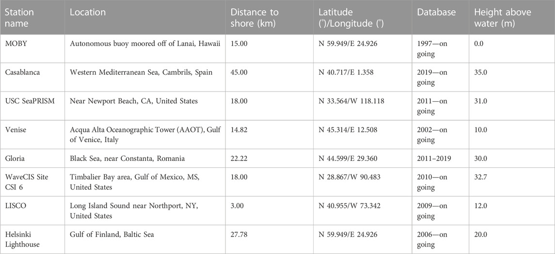
TABLE 1. Location and parameters of AERONET-OC sites.

In Section 2 the model (Gilerson et al., 2022) is briefly discussed, in Section 3 satellite and in situ data are described and results are presented in Section 4. Conclusions are provided in Section 5.

2 Main relationships in the estimation of uncertainties

A brief description of the model from Gilerson et al., 2022, is given here for the convenience of the reader. The main radiometric quantity in the processing of satellite data is the remote sensing reflectance, $R_{rs}$, which is defined as the ratio of the water-leaving radiance to the downwelling irradiance at the sea surface, $R_{rs}\left(\lambda \right)=L_w\left(\lambda \right)/E_d\left(\lambda \right)$, where $L_w\left(\lambda \right)$ is the water leaving radiance, $E_d\left(\lambda \right)$ is the downwelling irradiance and $\lambda$ is the wavelength. The main relationship for the top of the atmosphere (TOA) total radiance, $L_t\left(\lambda \right)$, can be represented as (Gordon and Wang, 1994)

${\mathit{L}}_{\mathit{t}}\left(\lambda \right)={\mathit{L}}_{\mathit{r}}\left(\lambda \right)+{\mathit{L}}_{\mathit{a}}\left(\lambda \right)+{\mathit{L}}_{\mathit{g}}\left(\lambda \right)+\mathit{t}\left(\lambda \right){\mathit{L}}_{\mathit{w}}\left(\lambda \right)(\mathrm{1a})$

where $L_r\left(\lambda \right)$ is due to the Rayleigh scattering and surface effects, $L_a\left(\lambda \right)$ is due to the aerosol scattering and Rayleigh-aerosol interaction, $L_g\left(\lambda \right)$ is due to the Sun glint from the water surface, $L_w\left(\lambda \right)$ is due to the water leaving radiance and $t\left(\lambda \right)$ is the diffuse transmittance of light from the water surface to the TOA. $L_t\left(\lambda \right)$ measured at the satellite sensor at 3 × 3 or more pixels has uncertainties due to all of these components in addition to vicarious calibration and sensor noise. It is important to emphasize that in the recording process $L_t\left(\lambda \right)$ already contains uncertainties from all its components in Eq. 1a because of the spatial variability of these components in the pixels of study. These include uncertainties from the water spatial variability, which as was shown by Gilerson et al., 2022, are not negligible in coastal areas. In the process of retrieval of the water leaving radiance, $L_r\left(\lambda \right)$, $L_a\left(\lambda \right)$, $L_g\left(\lambda \right)$ and $t\left(\lambda \right)$ are modeled and radiances are subtracted from the measured $L_t\left(\lambda \right)$, which introduces another set of uncertainties between actual and modeled radiances and transmittance coefficients:

${\mathit{L}}_{\mathit{w}}\left(\lambda \right)=\left({\mathit{L}}_{\mathit{t}}\left(\lambda \right)-{\mathit{L}}_{\mathit{r}}\left(\lambda \right)-{\mathit{L}}_{\mathit{a}}\left(\lambda \right)-{\mathit{L}}_{\mathit{g}}\left(\lambda \right)\right)/\mathit{t}\left(\lambda \right),(\mathrm{1b})$

In the model, $L_r\left(\lambda \right)$ was further divided into radiance from the Rayleigh scattering $L_R\left(\lambda \right)$ in the atmosphere and reflectance from the ocean surface:

${\mathit{L}}_{\mathit{r}}\left(\lambda \right)={\mathit{L}}_{\mathit{R}}\left(\lambda \right)+\mathit{t}\left(\lambda \right){\mathit{L}}_{\mathit{s}\mathit{u}\mathit{r}\mathit{f}}\left(\lambda \right),(\mathrm{1c})$

where $L_{surf}\left(\lambda \right)=L_{sky}\left(\lambda \right)*\rho$, $L_{sky}\left(\lambda \right)$ is the sky radiance and $\rho$ is the reflectance coefficient from the water surface. While usually in the satellite atmospheric correction procedure averaged surface effects are considered as a part of $L_r\left(\lambda \right)$ (Cox and Munk, 1954; Gordon and Wang, 1992), in this model they are considered separately because of differences in the spectra of $L_R\left(\lambda \right)$ and $L_{surf}\left(\lambda \right)$. Additionally, each satellite image captures a specific snapshot of the ocean, where the actual spatial average of the light field reflected from the wave facets may not exactly match the average predicted by the VRT model.

Uncertainties from all components included in Eq. 1a, 1b, 1c in the recording of the signal and in the retrieval process need to be taken into account. After normalizing radiances by the downwelling irradiance, $E_d\left(\lambda \right)$, the uncertainty in remote sensing reflectance $\sigma$ in sr⁻¹ can be determined from:

${\mathit{\sigma }}^{\mathbf{2}}=\left({\mathit{\sigma }}_{\mathit{t}}^{\mathbf{2}}+{\mathit{\sigma }}_{\mathit{R}}^{\mathbf{2}}+{\mathit{\sigma }}_{\mathit{a}}^{\mathbf{2}}+{\mathit{\sigma }}_{\mathit{g}}^{\mathbf{2}}\right)/{\mathit{t}}^{\mathbf{2}}+{\mathit{\sigma }}_{\mathit{s}\mathit{u}\mathit{r}\mathit{f}}^{\mathbf{2}}+{\mathit{\sigma }}_{\mathit{w}\mathit{a}\mathit{t}\mathit{e}\mathit{r}}^{\mathbf{2}}+{\mathit{\sigma }}_{\mathit{n}\mathit{o}\mathit{i}\mathit{s}\mathit{e}}^{\mathbf{2}}(2)$

Variances for the quantities at TOA ${\sigma }_t^2$, ${\sigma }_R^2$, ${\sigma }_a^2$, ${\sigma }_g^2$ are divided by $t^2$ in accordance with Eq. 1a, 1b, 1c. It was shown (Herrera-Estrella, et al., 2021) that estimated ${\sigma }_{noise}$ for the VIIRS sensor (Qi, et al., 2017; Xiong, et al., 2020) is significantly smaller than the total uncertainties $\sigma \left(\lambda \right)$ (Moore et al., 2015). OLCI ${\sigma }_{noise}$ (based on S3 OLCI Cyclic Performance Report, 2021) is of the same order (0.4*10^–4 sr⁻¹ at 412 nm and slightly lower for other bands) and will thus not be considered further. As before for VIIRS, OLCI ${\sigma }_R^2$, ${\sigma }_a^2$, ${\sigma }_g^2$ and ${\sigma }_{surf}^2$ contain uncertainties due to both natural variability inside the set of pixels and uncertainties due to modeling inaccuracies, while ${\sigma }_t^2$ is at least partially due to the vicarious calibration. It can also include other systematic errors due to detectors, polarization effects, stray light, etc., but these errors are not included in the model.

As one of the main assumptions of the model, all standard deviation components in Eq. 2 except ${\sigma }_t$ were, as a first approximation, considered proportional to the corresponding mean values of the normalized radiances with proportionality coefficient k:

${\mathit{\sigma }}^{\mathbf{2}}=\left({\mathit{\sigma }}_{\mathit{v}\mathit{c}}^{\mathbf{2}}+{\left({\mathit{k}}_{\mathit{R}}{\mathit{L}}_{\mathit{R}}/{\mathit{E}}_{\mathit{d}}\right)}^{\mathbf{2}}+{\left({\mathit{k}}_{\mathit{a}}{\mathit{L}}_{\mathit{a}}/{\mathit{E}}_{\mathit{d}}\right)}^{\mathbf{2}}+{\left({\mathit{k}}_{\mathit{g}}{\mathit{L}}_{\mathit{g}}/{\mathit{E}}_{\mathit{d}}\right)}^{\mathbf{2}}\right)/{\mathit{t}}^{\mathbf{2}}+{\left({\mathit{k}}_{\mathit{S}}\mathit{S}*\mathit{\rho }\right)}^{\mathbf{2}}+{\left({\mathit{k}}_{\mathit{R}\mathit{r}\mathit{s}}\mathit{R}\mathit{r}\mathit{s}\right)}^{\mathbf{2}}(3)$

where ${\sigma }_{vc}\left(\lambda \right)$ = ${\sigma }_{gains}\left(\lambda \right)L_t\left(\lambda \right)/E_d\left(\lambda \right)$, and ${\sigma }_{gains}\left(\lambda \right)$ is the standard deviation of the system vicarious calibration gains (unitless) for OLCI from EUMETSAT processing. Additionally,

${\mathit{L}}_{\mathit{R}}\left(\mathit{\lambda }\right)={\mathit{F}}_{\mathbf{0}}\left(\mathit{\lambda }\right){\mathit{\tau }}_{\mathit{R}}\left(\mathit{\lambda }\right)\ast \mathbf{0.75}\ast \frac{\mathbf{1}+{\mathit{cos}}^{\mathbf{2}}\mathit{\Theta }}{\mathbf{4}\mathit{\pi }\mathit{cos}\mathit{\theta }}(\mathrm{4a})$

${\mathit{L}}_{\mathit{a}}\left(\mathit{\lambda }\right)=\frac{{\mathit{\omega }}_{\mathbf{0}}\left(\mathit{\lambda }\right){\mathit{F}}_{\mathbf{0}}\left(\mathit{\lambda }\right){\mathit{\tau }}_{\mathit{a}}\left(\mathit{\lambda }\right){\mathit{P}}_{\mathit{a}}}{\mathbf{4}\mathit{\pi }\mathbf{cos}\mathit{\theta }}(\mathrm{4b})$

${\mathit{L}}_{\mathit{g}}\left(\mathit{\lambda }\right)={\mathit{F}}_{\mathbf{0}}\left(\mathit{\lambda }\right){\mathit{T}}_{\mathbf{0}}\left(\mathit{\lambda }\right)\mathit{T}\left(\mathit{\lambda }\right)\ast \mathbf{0.005}(\mathrm{4c})$

${\mathit{E}}_{\mathit{d}}\left(\mathit{\lambda }\right)={\mathit{F}}_{\mathbf{0}}\left(\mathit{\lambda }\right){\mathit{t}}_{\mathbf{0}}\left(\mathit{\lambda }\right)\mathbf{cos}{\mathit{\theta }}_{\mathbf{0}}(\mathrm{4d})$

${\mathit{L}}_{\mathit{s}\mathit{u}\mathit{r}\mathit{f}}\left(\mathit{\lambda }\right)={\mathit{\rho }\mathit{L}}_{\mathit{s}\mathit{k}\mathit{y}}\left(\mathit{\lambda }\right);\mathit{S}\left(\mathit{\lambda }\right)=\frac{{\mathit{L}}_{\mathit{s}\mathit{k}\mathit{y}}\left(\mathit{\lambda }\right)}{{\mathit{E}}_{\mathit{d}}\left(\mathit{\lambda }\right)}(4e)$

In Eq. 4a $F_0\left(\lambda \right)$ is the extraterrestrial irradiance, $\theta$ is the sensor zenith angle, $\mathrm{\Theta }$ is the scattering angle, the angle between solar and viewing directions; in Eq. 4b ${\omega }_0\left(\lambda \right)$ is the single scattering albedo, $P_a$ is the scattering function for aerosols; in (5c) $T_0\left(\lambda \right)$, $T\left(\lambda \right)$ are the direct transmittance coefficients for TOA to surface and surface to TOA respectively, and 0.005 is the threshold for glint detection; $L_{GN}$, in sr⁻¹ (Wang and Bailey, 2001); in Eq. 4d ${\theta }_0$ and $t_0\left(\lambda \right)$ are the Sun zenith angle and the corresponding diffuse transmittance; in Eq. 4e a representative normalized sky reflectance, $S=L_{sky}/E_d$, was simulated by the VRT RayXP code (Tynes et al., 2001) for the Sun zenith angle ${\theta }_0=42°$ at a viewing zenith angle of 40°, with ${\tau }_a\left(443\right)$ and Angstrom coefficient average values for each specific area based on the satellite processing values given below in Table 2. Aerosol radiance in Eq.4b was determined assuming ${\omega }_0$ = 1 for all wavelengths, with aerosol optical thickness values and the Angstrom coefficient derived from satellite imagery, and with the phase function (PF) equal to 0.3 corresponding to the scattering angle around 120°. The water component ${\sigma }_{water}$ was expressed directly proportional to the remote sensing reflectance $R_{rs}$.

TABLE 2

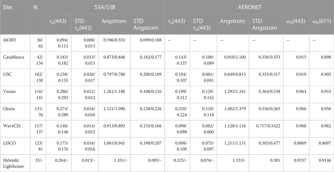
TABLE 2. Average atmospheric parameters at the sites of study determined from satellite and AERONET retrievals.

Equation 3 includes OLCI S3A and 3B system vicarious calibration uncertainties ${\sigma }_{vc}$, where sensor gains are determined by the comparison of the atmospherically corrected water leaving radiance with in situ measurements at the MOBY site (Franz et al., 2007). ${\sigma }_{gains}\left(\lambda \right)$ are included as constant spectra with values ${\sigma }_{gains}\left(\lambda \right)$ = [0.014210, 0.014000, 0.013206, 0.007822, 0.004042] for S3A and ${\sigma }_{gains}\left(\lambda \right)$ = [0.012342, 0.012278, 0.011843, 0.007769, 0.003752] for S3B for corresponding wavelengths [412.5, 442.5, 490, 560, 665] (EUMETSAT, 2020). Data processing was carried out first without ${\sigma }_{vc}\left(\lambda \right)$ in Eq. 3 to understand the contributions of other components to the total $\sigma \left(\lambda \right)$ and then with ${\sigma }_{vc}\left(\lambda \right)$ included.

For each available matchup between satellite and AERONET-OC measurements, all radiance spectra in Eqs 4a, 4b, 4c, 4d were calculated, then spectra were averaged over the total number of available measurements. Mean spectra were then used in the fitting procedure based on Eq. 3, and on mean $R_{rs}\left(\lambda \right)$ to determine the contribution of each component to the total ${\sigma }^2\left(\lambda \right)$. Because of the shorter period of operation of OLCI on S3A and especially on S3B than of VIIRS, the number of matchups was significantly smaller than for VIIRS and differences in wind speeds were not considered. In addition, outliers in uncertainties spectra or unusual spectra not typical for respective water areas from the AERONET-OC (in-situ) data were removed from matchups since they had a significant impact on results given the small number of total data points.

$\sigma \left(\lambda \right)$ was calculated from the comparison of satellite data with the corresponding AERONET-OC station data in all bands as

$\mathit{R}\mathit{M}\mathit{S}\mathit{D}=\sqrt{\frac{{\displaystyle \sum }_{\mathit{i}=\mathbf{1}}^{\mathit{N}}{\left({\mathit{R}}_{\mathit{r}{\mathit{s}}_{\mathit{s}\mathit{a}\mathit{t}}}^{\mathit{i}}-{\mathit{R}}_{\mathit{r}{\mathit{s}}_{\mathit{i}\mathit{n}-\mathit{s}\mathit{i}\mathit{t}\mathit{u}}}^{\mathit{i}}\right)}^{\mathbf{2}}}{\mathit{N}}}(5)$

with $\sigma \left(\lambda \right)$ = RMSD.

Biases were also calculated as

$\mathit{b}\mathit{i}\mathit{a}\mathit{s}=\frac{{\displaystyle \sum }_{\mathit{i}=\mathbf{1}}^{\mathit{N}}\left({\mathit{R}}_{\mathit{r}{\mathit{s}}_{\mathit{s}\mathit{a}\mathit{t}}}^{\mathit{i}}-{\mathit{R}}_{\mathit{r}{\mathit{s}}_{\mathit{i}\mathit{n}-\mathit{s}\mathit{i}\mathit{t}\mathit{u}}}^{\mathit{i}}\right)}{\mathit{N}}(6)$

Each of radiances in Eq. 4, has individual spectral variable(s) not repeated in other equations, so all spectra of uncertainties, which were considered proportional to these radiances, should be independent of each other. An optimization procedure was carried out in the same manner as in Gilerson et al., 2022 in MATLAB using the default trust-region-reflective algorithm (Coleman and Li, 1994; Coleman and Li, 1996) to determine the respective values of the k coefficients for MOBY and each AERONET-OC site based on the spectra of the $\sigma \left(\lambda \right)$ components and their individual contribution to the total observed $R_{rs}$ variance ${\sigma }^2\left(\lambda \right)$ as described in Eq. 3. Spectral components were normalized before being used as inputs in the procedure, and results were averaged over 100 runs with random initial conditions to test the robustness of the solution against possible local minima. The normalization did not affect spectral shapes of components and was used to avoid small values of uncertainties, which can be not treated correctly in the fitting process. Once a solution was reached, all normalized k coefficients were then scaled back to their true scale values and were interpreted as an indication of the major contributing components to the total observed $R_{rs}$ variance ${\sigma }^2\left(\lambda \right)$.

Equation 3 can be alternatively presented as

${\mathit{\sigma }}^{\mathbf{2}}=\left[{\mathit{\sigma }}_{\mathit{v}\mathit{c}}^{\mathbf{2}}+{\left({\mathit{\sigma }}_{\mathit{R}}^{\mathbf{412}}\frac{{\mathit{L}}_{\mathit{R}}/{\mathit{E}}_{\mathit{d}}}{{\mathit{L}}_{\mathit{R}}^{\mathbf{412}}/{\mathit{E}}_{\mathit{d}}^{\mathbf{412}}}\right)}^{\mathbf{2}}+{\left({\mathit{\sigma }}_{\mathit{a}}^{\mathbf{412}}\frac{{\mathit{L}}_{\mathit{a}}/{\mathit{E}}_{\mathit{d}}}{{\mathit{L}}_{\mathit{a}}^{\mathbf{412}}/{\mathit{E}}_{\mathit{d}}^{\mathbf{412}}}\right)}^{\mathbf{2}}+{\left({\mathit{\sigma }}_{\mathit{g}}^{\mathbf{412}}\frac{{\mathit{L}}_{\mathit{g}}/{\mathit{E}}_{\mathit{d}}}{{\mathit{L}}_{\mathit{g}}^{\mathbf{412}}/{\mathit{E}}_{\mathit{d}}^{\mathbf{412}}}\right)}^{\mathbf{2}}\right]/{\mathit{t}}^{\mathbf{2}}+{\left({\mathit{\sigma }}_{\mathit{S}}^{\mathbf{412}}\frac{\mathit{S}}{{\mathit{S}}^{\mathbf{412}}}\right)}^{\mathbf{2}}+{\left({\mathit{\sigma }}_{{\mathit{R}}_{\mathit{r}\mathit{s}}}^{\mathbf{560}}\frac{{\mathit{R}}_{\mathit{r}\mathit{s}}}{{\mathit{R}}_{\mathit{r}\mathit{s}}^{\mathbf{551}}}\right)}^{\mathbf{2}}(7)$

where normalized radiance spectra $L_R/E_d$, etc. are divided by their values at 412 nm (at 560 nm for $R_{rs}$) and corresponding k coefficients are multipled by these values. Thus k coefficients are replaced by the standard deviation for each term at the reference wavelength, 412 and 560 respectively. In this case standard deviations at the reference wavelengths have clear physical interpretation and they can be conveniently compared for different terms.

3 Satellite and AERONET-OC data

3.1 OLCI data

OLCI S3A and S3B Collection 3 level 2 Full Resolution imagery (300 m spatial resolution by pixel, EUMETSAT, 2021) was downloaded from the EUMETSAT website for the period of January 2017 to July 2022 for S3A and from May 2018 to July 2022 for S3B for the areas of MOBY in Lanai, Hawaii and seven Aerosol Robotic Network for Ocean Color (AERONET-OC) sites: Casablanca, University of South California (USC), Venise, Gloria, WaveCIS, the Long Island Sound Coastal Observatory (LISCO) and the Helsinki Lighthouse (HLT) with locations shown in Figure 1.

FIGURE 1

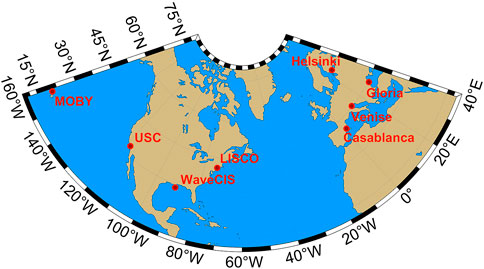
FIGURE 1. Areas of study: Global map showing MOBY area and all AERONET-OC stations used in this study.

Collection 3 was obtained using the extraction data base (EDB) workflow scripts (https://github.com/juanchossn/ThoMaS), and Level 2 SeaBASS - Ocean Colour Database (OCDB) format images were retrieved with a window size of 25 × 25 pixels centered on the previously named sites. Each level 2 file includes geophysical products of the atmosphere and ocean, such as aerosol optical thickness and Angstrom exponent at 865 nm, water-leaving reflectance at 412.5, 443.5, 490, 560, and 665 nm among others, sensor zenith angle, solar zenith angle, and quality flags. $R_{rs}\left(\lambda \right)$ is calculated dividing the water-leaving reflectance spectra by π.

OLCI Collection 3 level 2 operational water reflectance products are not corrected for the bidirectional reflectance distribution function (BRDF). The BRDF correction is not applied for historical reasons as the main users have typically been interested in coastal and inland waters where the standard open-ocean BRDF approach does not apply. Nevertheless, the BRDF correction was applied externally in this study to OLCI L2 products as it is necessary for the current analyses (Morel et al., 2002).

Pixels flagged by at least one of the following conditions were excluded: invalid flag, land, cloud (including ambiguous and marginal), coastline, high solar zenith angle larger than 70°, saturated flag, moderate or high glint, whitecaps, and atmospheric correction fail. It should be noted that this set of flags is slightly different from the set recommended for OLCI by EUMETSAT (EUMETSAT, 2022). A file is selected if at least half of the pixels in the set plus one was flag-free. Pixels used for matchup comparison were averaged over 5 spatial resolutions: 900, 1,500, 2,100, 3,900, and 5,100 m (3 × 3, 5 × 5, 7 × 7, 13 × 13, and 17 × 17 pixel boxes), centered at the AERONET-OC site (Hlaing et al., 2013). Average $R_{rs}\left(\lambda \right)$ and the standard deviation between pixels and geometry were recorded.

3.2 VIIRS data

VIIRS’s Satellite Level 2—Version 2018.0 imagery was downloaded, for the same areas, from the NASA Ocean Color website https://oceancolor.gsfc.nasa.gov (Gordon and Wang, 1994; Siegel et al., 2000; Bailey et al., 2010). Standard NASA Level 2 data files for VIIRS (with a pixel resolution of 750 m at nadir) include geophysical products of the atmosphere and ocean, such as aerosol optical thickness at 862 nm, remote sensing reflectance, $R_{rs}\left(\lambda \right)$, in the visible wavelengths 410, 443, 486, 551, and 671 nm, and the level 2 quality flags.

Pixels flagged by at least one of the following conditions were excluded: land, cloud, failure in atmospheric correction, stray light (except for LISCO), bad navigation quality, high or moderate glint, negative Rayleigh-corrected radiance, negative water-leaving radiance, viewing angle larger than 60°, and solar zenith angle larger than 70°. A file is selected if at least half of the pixels in the set plus one was flag-free. Pixels used for matchup comparison were averaged over 3 spatial resolutions: 2,250, 3,750, and 5,250 m (3 × 3, 5 × 5, and 7 × 7 pixel boxes), centered at the AERONET-OC site (Hlaing et al., 2013; Gilerson et al., 2022). Average $R_{rs}\left(\lambda \right)$ and the standard deviation between pixels, geometry, and radiance were recorded.

3.3 AERONET-OC data

The ocean color component of the Aerosol Robotic Network (AERONET-OC) was implemented to support long-term ocean color investigations by collecting normalized water-leaving radiance and aerosol optical depth data using the SeaPRISM autonomous radiometer systems CE-318/CE-318T (CIMEL Electronique, France) deployed on offshore fixed platforms (Zibordi et al., 2009; Zibordi et al., 2021). SeaPRISM systems are used to retrieve atmospheric optical thickness and other atmospheric parameters, and modified to perform radiance measurements with a full-angle field of view of 1.2° to determine the total radiance from the sea surface, $L_t^A$ (λ), and the sky radiance, $L_{sky}^A$ (λ), as a function of solar zenith angle, sensor viewing angle, and azimuth angle relative to the Sun (Zibordi et al., 2009).

The normalized water leaving radiances, $L_w^A$, which were measured and then calculated in accordance with AERONET-OC protocols with the BRDF correction based on the open ocean approach (Zibordi et al., 2009; Zibordi et al., 2021), were downloaded for the sites mentioned above from the AERONET-OC website and were converted into remote sensing reflectance at the wavelengths 412, 443, 488, 551(or 560 when available), and 667 nm available on the CE-318 sunphotometers.

Several AERONET-OC stations had 551 nm band for the whole period of OLCI operation, some of them had new sensor heads with 560 nm band for some part of this period. Considering water type variability between sites and at sites themselves, introduction of some algorithm of band shift most likely would have introduced more uncertainties, so available data at AERONET-OC stations at 551 (or 560) nm were used without changes. SNPP VIIRS also has 551 nm band. Tests were conducted by changing the value of $R_{rs}$ (551) by 5% to simulate a band-shift effect, and the results of the spectral decomposition were not noticeably affected.

The aerosol optical depth, aerosol inversions, and ocean color data used in this analysis are version 3 level 1.5 data, which has been cloud-screened and quality controlled to ensure the accuracy of the data. All matchups were observed within a ±2 h window between satellite overpass and in situ observation (Zibordi et al., 2009; Zibordi et al., 2021). More detailed information on AERONET-OC sites is listed in Table 1.

3.4 The Marine Optical BuoY (MOBY) data

MOBY (Marine Optical BuoY) is an autonomous buoy anchored offshore of Lanai, Hawaii. Its radiometry data is used by the NASA—OBPG and EUMETSAT as part of their ocean color validation and vicarious calibration activities (Clark et al., 1997). On each day of deployment, it collects several measurements of upwelling radiance from sensors on its underwater arms (at approximately 1, 5, and 9 m depth) and downwelling irradiance from sensors on its underwater arms as well as at the surface (Voss et al., 2017).

From the MOBY “gold” directory, data from deployments 266 to 272 (2019–2021) was collected for OLCI S3A and S3B, and 249 to 270 (2012–2021) for VIIRS-NPP. Normalized water-leaving radiance calculated from the top sensor and bottom sensor corrected for BRDF is used here because it has the larger available dataset. “Good” and “questionable” data were used to match up with satellite data. Matchups with more than 5 percent differences were excluded from the analysis. MOBY data that matched the bands from satellite sensors was collected with ±2 h of the satellite overpass.

Main atmospheric parameters at the studied sites determined from AC processing and AERONET retrievals are provided in Table 2. Absorbing aerosols were noticeable at several sites with the average ${\omega }_0$ values usually above 0.9 and even below 0.9 at LISCO, but spectral dependence was small.

4 Results: Spectral components of uncertainties

Mean $R_{rs}\left(\lambda \right)$ spectra from the MOBY site and AERONET-OC stations based on in-situ measurements are shown in Figure 2A; waters were clear or moderately clear at MOBY, Casablanca and USC with $R_{rs}$ (443)> $R_{rs}$ (551), moderately eutrophic at Venise, Gloria and WaveCIS with $R_{rs}$ (443)< $R_{rs}$ (551) and more eutrophic at LISCO and HLT with also low $R_{rs}$ (412) $R_{rs}\left(\lambda \right)$. standard deviations are shown in Figure 2B. Corresponding $\sigma \left(\lambda \right)$ spectra are shown in Figures 2C–E for OLCI S3A, S3B and VIIRS respectively. They have different shapes for different stations with highest values in the blue. Uncertainties are very similar for S3A and S3B, some small differences here and below are due to the different number of matchups and conditions of individual matchups. Uncertainties for VIIRS are spectrally similar to OLCI uncertainties, they are approximately the same in magnitude at MOBY and about 50% higher at other stations. Biases are shown in Figures 2F–H and are very similar for OLCI S3A and S3B with moderate spectral dependence. OLCI biases are also in the same range as for VIIRS and spectrally differ mostly at 412–443 nm. There were very small number of matchups between OLCI S3B and the Helsinki AERONET-OC station, and these results are not presented here nor below.

FIGURE 2

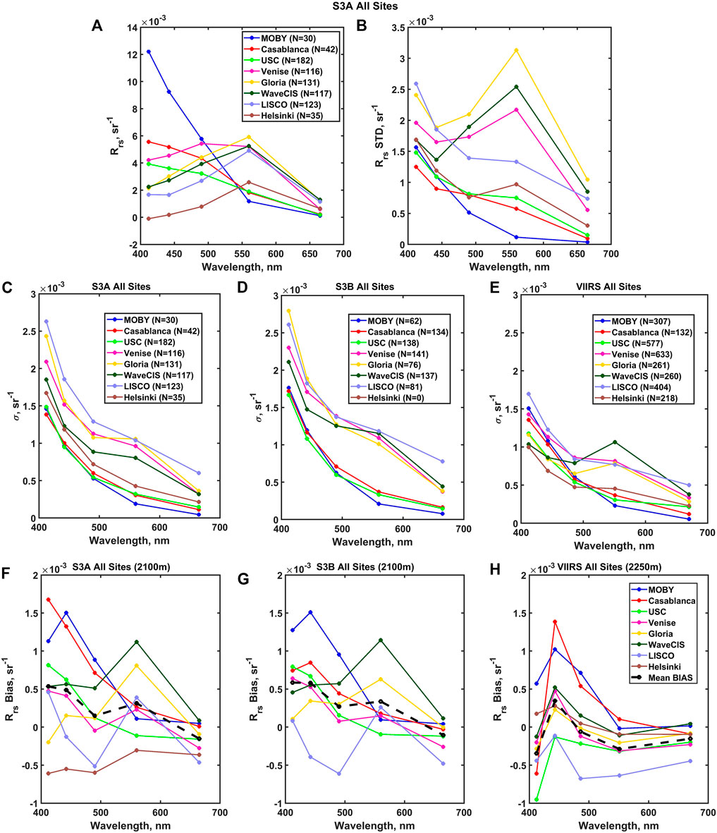
FIGURE 2. (A) Mean $R_{rs}\left(\lambda \right)$ spectra from AERONET-OC, (B) standard deviations of $R_{rs}\left(\lambda \right)$ for matchups with S3A. (C, D, and E) corresponding uncertainties spectra $\sigma \left(\lambda \right)$ for all areas of study, S3A, 3B and VIIRS respectively, (F, G, and H) biases for S3A, S3B and VIIRS.

Spectra for all components from Eq. 3 normalized to their maxima are shown for all stations in Figure 3 and these spectra were used in the fitting procedure. In accordance with Eq. 3 ${\sigma }_R$, ${\sigma }_a$, ${\sigma }_g$ are divided by the spectrum of the diffuse transmittance t for the propagation of light from the surface to TOA. The normalized spectra for the Rayleigh scattering and glint are the same for all stations, while spectra for the total $\sigma \left(\lambda \right)$, for aerosols and $R_{rs}\left(\lambda \right)$ components are different.

FIGURE 3

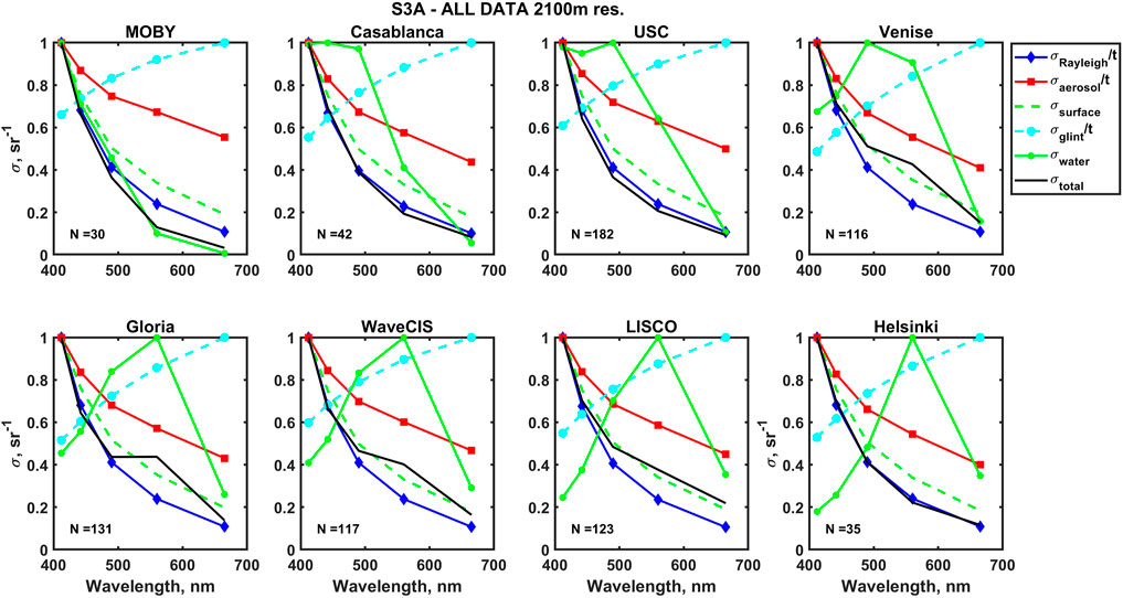
FIGURE 3. Normalized spectra for all sites (7 × 7 pixels, 2,100 m resolution), OLCI S3A.

Spectra for surface effects are slightly different for different stations because of the small difference in the aerosol parameters used for their calculations. Rayleigh scattering and surface effects spectra are both related to the sky spectra, but the former is divided by the spectrum of the diffuse transmittance t and the latter was simulated based on the composition of Rayleigh and aerosol scattering, which makes these spectra distinct from each other.

Results of fitting are presented in Figure 4 for S3A and S3B. Because of the similarity of the total uncertainties’ spectra for S3A and S3B, it is not surprising that spectral components are also similar. For most of the stations fitted spectra (dash black lines) match well solid lines of total uncertainties spectra confirming that most likely all relevant components were taken into account. For all stations the main component of $\sigma \left(\lambda \right)$ is Rayleigh scattering. Glint and surface effects are small, and aerosol contributions are noticeable for LISCO only. With some differences, water variability terms (green solid lines) are quite pronounced, especially at coastal stations, which is usually not considered in the uncertainties budget.

FIGURE 4

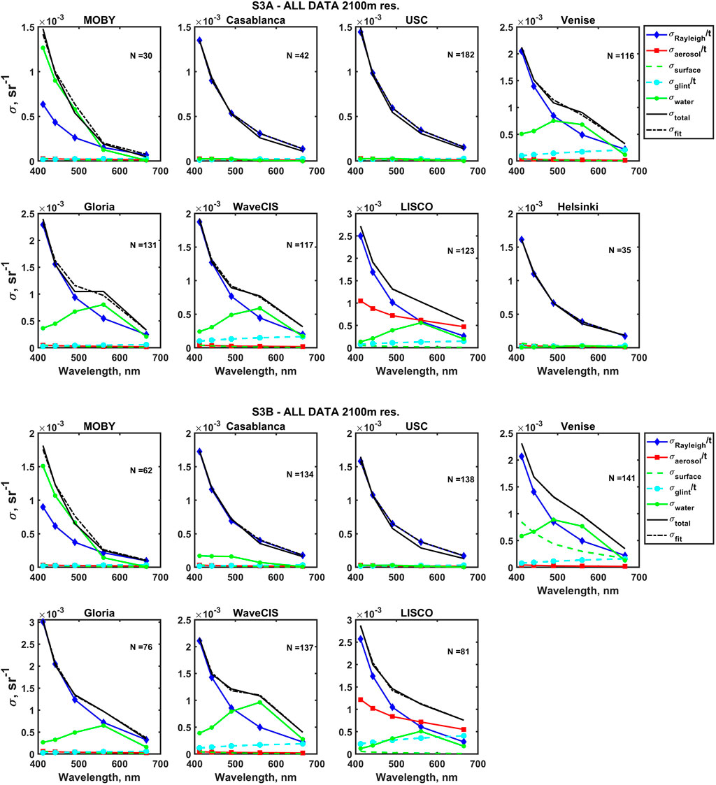
FIGURE 4. Results of fitting for all areas of study for OLCI S3A and S3B. Total uncertainty is the solid black line, and the fitted curve is dashed black line.

Results are very similar for SNPP VIIRS with relatively stable ${\sigma }_R^{412}=\left(0.9-1.4\right)*{10}^{-3}s{r}^{-1}$ as seen in Figure 5. It should be emphasized that in Figures 4, 5 standard deviations are presented, while the fitting process is carried out on variances, so even small differences in the values of spectral components in Figures 4, 5 are amplified in the fitting procedure.

FIGURE 5

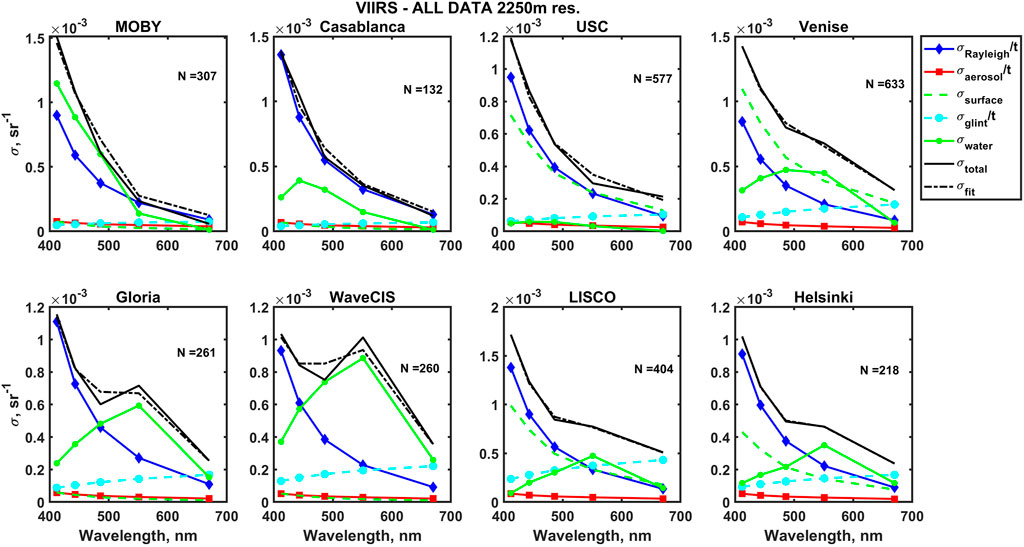
FIGURE 5. Results of fitting for VIIRS same stations. Total uncertainty is the solid black line and the fitted curve is dashed black line.

Since the validity of the assumption that the uncertainties spectra are proportional to the spectra of the components themselves can be less accurate for aerosols than for other components, it is possible that the optimization procedure underestimates the contribution of the aerosol component to the total uncertainties. Generally, however, the aerosol uncertainty levels are consistent with their estimations or slightly below them (Wang, 2007; Gao et al., 2022), where they are at the level of 10^–4–4*10^–4 sr⁻¹. LISCO station has a pronounced aerosol component for both OLCI S3A and S3B, which is not visible in VIIRS. It can be partially due to the different atmospheric correction processes in OLCI and VIIRS, as well as different number of matchups for these sensors. Some inaccuracies in spectral composition can also be present after optimization because of the similarity of some of the spectra (cf. Rayleigh and surface effects spectra).

For both OLCI and VIIRS sensors the water variability term (solid green line) is very pronounced at the MOBY site. This can be partially due to the similarity of $R_{rs}$ and Rayleigh spectra but is probably also related to the temporal variability of $R_{rs}$ at the site since, as was shown in Herrera-Estrella et al., 2021, spatial variability of $R_{rs}$ is very small in such waters. Also, Brown et al. (2007) estimated uncertainties for upwelling radiance $L_u$ (412) for “good” days at 2.4% and 4.7% in general. Assuming similar uncertainties for the downwelling irradiance and $R_{rs}\left(412\right)$ = 0.012 sr⁻¹, related ${\sigma }^{412}$ can be about 6*10^–4 sr⁻¹, which at least partially justifies large uncertainty proportional to the $R_{rs}$ at the MOBY site, well visible in Figures 4, 5 as a green solid line.

While results have many similarities between VIIRS and OLCI sensors, some differences are present due to higher uncertainties at OLCI, differences in atmospheric correction algorithms, imperfectness of the fitting approach for the separation of components, especially with similar spectra, and the different number of matchups. Thus, for example, at the LISCO site the shape of the surface and aerosol spectra seemed to switch. For S3A/B, aerosol spectra are close to exponential with ${\sigma }_a\left(412\right)\approx$ 10^–3, and the surface spectra are almost flat and near zero. For VIIRS, the exact opposite happens: the surface spectrum is close to exponential with a magnitude of 10^–3 and the aerosol spectrum is flat and near zero. Interestingly, at the Venise site there is a big surface contribution for S3B, but not for S3A. Glint effects are more visible in VIIRS than in OLCI S3A/B.

Standard deviations ${\sigma }^{412}$ and ${\sigma }^{551}$ retrieved in the fitting procedure for both OLCI sensors and VIIRS for all areas are shown in Figure 6 as a function of spatial resolution, starting from 3 × 3 pixels (900 × 900 m) to 17 × 17 pixels (5100 × 5100 m) for OLCI and from 3 × 3 pixels (2250 × 2250 m) to 7 × 7 pixels (5250 × 5250 m) for VIIRS. Fully in accordance with Figures 4, 5, with exception of Venise for VIIRS, the standard deviations for aerosol, glint and surface effects components are much smaller than for the Rayleigh scattering component, while water variability through ${\sigma }^{551}$ is pronounced for most of coastal sites. For aerosols, glint, surface effects and water variability ${\sigma }^{412}$, ${\sigma }^{551}$ are in the same range for both OLCI and VIIRS; however, they are different for the Rayleigh component, as will be discussed in further detail below. Some dependence of these standard deviations on the spatial resolution as well as some differences between OLCI S3A and S3B are not systematic and are most likely due to the different number and timing of matchups, which are not properly averaged over the relatively small number of observations. Rayleigh component ${\sigma }_R^{412}$ for OLCI and VIIRS are compared in Figure 7. It can be clearly seen that these standard deviations differ in a small range for VIIRS and in a much larger range for OLCI sensors. At the MOBY site OLCI ${\sigma }_R^{412}$ values are similar to VIIRS ${\sigma }_R^{412}$ values but are instead higher at other stations and consistently so for both OLCI 3A and 3B. It can be also noticed that these OLCI ${\sigma }_R^{412}$ values, with some exceptions, tend to vary in accordance with the latitude of the stations, as can be seen roughly in Figure 1; Table 1, which leads to their possible dependence on the solar zenith angle, mean values for which are provided in Table 3 together with sensor zenith angle. In Zibordi et al., 2022 it was also shown that dependence of uncertainties exists for the sensor zenith angle as well; however, this is not apparent in VIIRS data. Both these effects merit further study. It should be also noticed that comparison of processing of OLCI data using EUMETSAT and NOAA MSL12 algorithms (Mikelsons et al., 2022) showed smaller $R_{rs}$ uncertainties for MSL12, which can assume that larger OLCI uncertainties than for VIIRS shown above are associated with the processing algorithm and not with design features of the instruments.

FIGURE 6

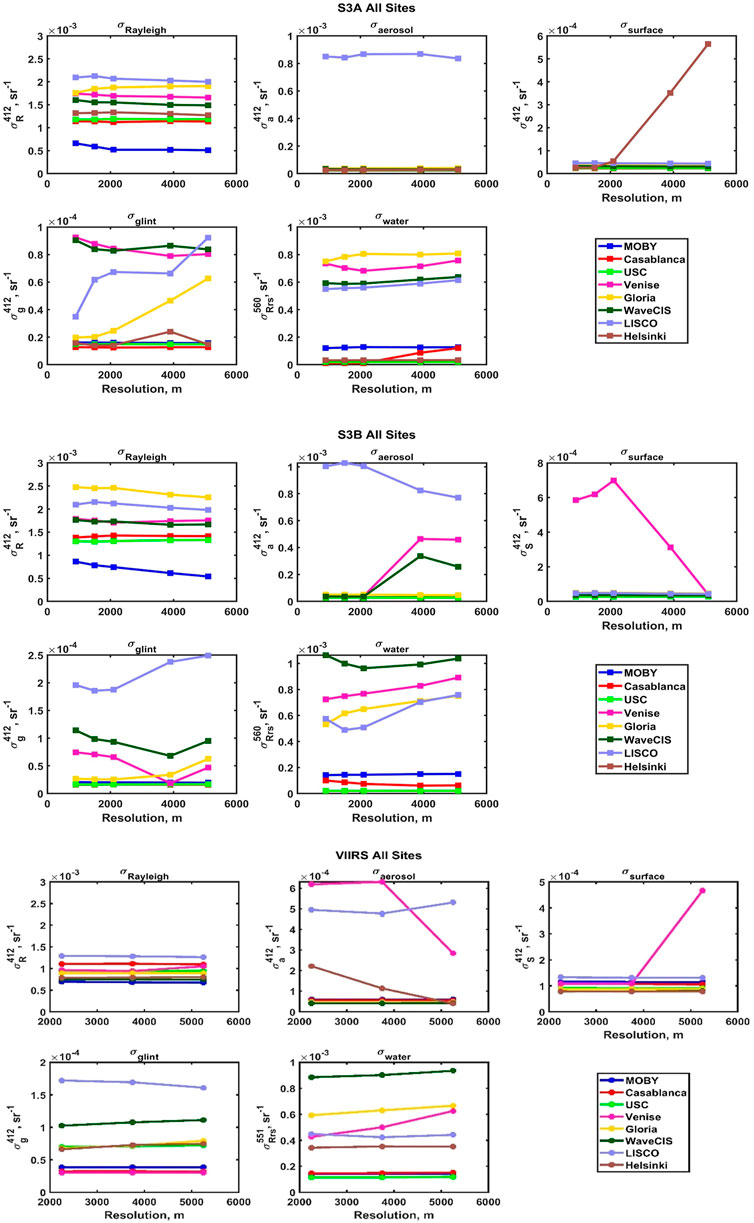
FIGURE 6. Proportionality coefficients in Eq. 7 in the form of standard deviations at referenced wavelengths.

FIGURE 7

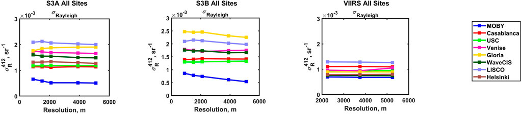
FIGURE 7. Comparison of ${\sigma }_R^{412}$ for OLCI S3A and S3B and VIIRS.

TABLE 3

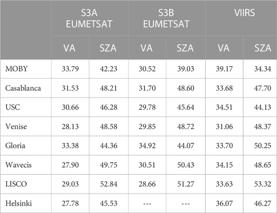
TABLE 3. Viewing (VA) and solar zenith (SZA) angles (in degrees) at the areas of study.

In Gilerson et al., 2022 it was shown that ${\sigma }_R^{412}$ = 1*10^–3 sr⁻¹ corresponds approximately to the uncertainty in the Rayleigh optical thickness (ROT) of about 1.5%. The uncertainty in ROT was estimated as the ratio of determined Rayleigh uncertainties spectra to the average Rayleigh radiance component at TOA normalized by the downwelling irradiance. This number remains the same for OLCI in case of the MOBY site. Higher uncertainties for coastal sites are most likely associated with other reasons related to the processing algorithms (for example, higher uncertainties in modeling of the surface pressure, which is directly related to the estimation of ROT).

Following the hypothesis in Gilerson et al., 2022 that Rayleigh components of uncertainties are related to the standard deviation of gains ${\sigma }_{gains}\left(\lambda \right)$ during the vicarious calibration at the MOBY site, the fitting procedure was repeated with vicarious calibration terms included as it was given in Eq. 3 and ${\sigma }_{gains}\left(\lambda \right)$ below it, with results shown in Figure 8 for both OLCI and VIIRS sensors. As discussed in Gilerson et al., 2022, the standard deviation of gains ${\sigma }_{gains}\left(\lambda \right)$ is mostly related to the variability of atmospheric parameters and thus should not depend on the sensor. OLCI S3B ${\sigma }_{gains}\left(\lambda \right)$ are very close to the ones from VIIRS, while OLCI S3A ${\sigma }_{gains}\left(\lambda \right)$ are about 15% higher. Based on the similarity of the total uncertainties’ spectra and their spectral components for OLCI S3A and S3B as shown in Figures 2, 4, this difference in ${\sigma }_{gains}\left(\lambda \right)$ (see values for S3A and S3B in Section 2) does not have an immediate explanation.

FIGURE 8

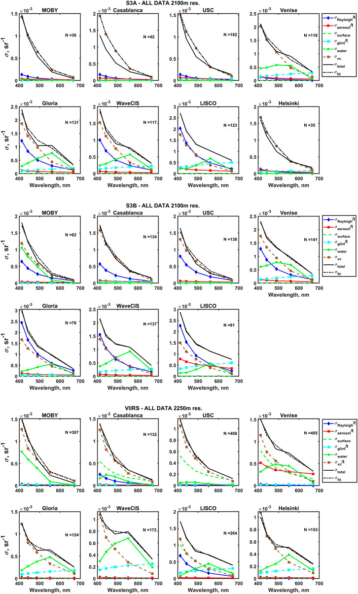
FIGURE 8. Results of fitting for all areas of study for OLCI S3A, S3B and VIIRS with VC term included.

While for VIIRS ${\sigma }_{vc}$/t replaced most of Rayleigh components, for the OLCI S3B sensor an additional Rayleigh component remained, which correlated with higher total uncertainties for OLCI than for VIIRS. The reason for additional OLCI uncertainties is not obvious, but it is probably related to some features in the processing algorithms for these sensors. For OLCI S3A, as for VIIRS, ${\sigma }_{vc}$/t replaced most of Rayleigh components shown in Figure 4, with the obvious exception of the Casablanca station where, for reasons yet unclear, the fitted curve was higher than the spectrum of the total uncertainties. Other components remain similar to how they were in Figure 4 for both OLCI sensors.

Melin, 2022 compared satellite and AERONET-OC data for the European sites and for several sensors launched before OLCI and found that for specific stations the spectra of uncertainties from different sensors are close to each other, thus supporting the hypothesis in Gilerson et., 2022 that such uncertainties are mostly due to the variability of atmospheric parameters (or their calculation).

Zibordi et al., 2022 evaluated uncertainties for the European sites over the period of the so-called “Tandem Phase,” with Sentinel-3B and Sentinel-3A flying just 30 s apart on the same orbit, and showed spectral median percent differences lower than ±1% in the 412–560 nm interval, much lower than when the sensors were on the same orbit but with the nominal phase difference. This is also very consistent with the hypothesis of a dependence of the uncertainties on the atmospheric parameters (or their calculation), since these should be almost the same for both satellites in the Tandem Phase configuration.

As discussed in Gilerson et al., 2022, uncertainties related to AERONET-OC measurements (Gergely and Zibordi, 2014), are about 4 times smaller than the total uncertainties at all stations and thus play a small role in the total uncertainties budget. With OLCI uncertainties typically higher than for VIIRS, this is also true for the evaluation of OLCI sensors data. However, if it will be possible to make the Rayleigh component contribution to the total uncertainties smaller, remaining uncertainties can be similar to the ones from AERONET-OC and the issue will require more attention.

In Figure 9 the spectra of $∆R_{rs}={R_{rs}}_{sat}^i-{R_{rs}}_{in-situ}^i$ are shown for MOBY and two AERONET-OC sites in the first column, with bias subtracted in the second column and the histogram of the second column data at 412 nm in the third column. Satellite data are from OLCI S3A. After correction for biases the $∆R_{rs}$ distribution is clearly almost symmetrical and close to normal for the open ocean MOBY and coastal Venise and LISCO sites, confirming that negative uncertainties values are for the most part not associated with absorbing aerosols.

FIGURE 9

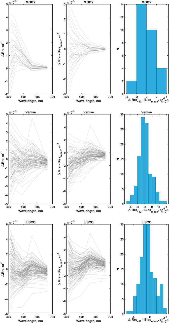
FIGURE 9. Analysis of the S3A $∆R_{rs}$ distribution for MOBY, Venise and LISCO sites. First column: all $∆R_{rs}$, second column: all $∆R_{rs}$—mean bias for the station, third column: histogram of all $∆R_{rs}$– mean bias for the station at 412 nm.

In Figure 10 ${\sigma }_{vc}$ spectra for OLCI S3A/B and VIIRS calculated as ${\sigma }_{vc}\left(\lambda \right)$ = ${\sigma }_{gains}\left(\lambda \right)L_t\left(\lambda \right)/E_d\left(\lambda \right)$ at the MOBY site are compared with Rayleigh components determined from the fitting procedure for these sensors also for the MOBY site and shown in Figures 4, 5. For OLCI S3B and VIIRS ${\sigma }_{vc}$ spectra are very similar to each other and to Rayleigh components. The differences are larger for S3A, which are most likely due to the inaccuracies of measurements, different number of matchups, etc., considering that all other spectral characterisitics related to $R_{rs}$ and uncertanties are very similar. This again confirms that Rayleigh uncertainties spectra determined in this work are close to ${\sigma }_{vc}$ at the MOBY site and represent a significant part of Rayleigh uncertainties at other sites with remaining differences can be probably mitigated with advanced processing algorithms. To remind, as was shown in Gilerson et al., 2022, for VIIRS ${\sigma }_{vc}$ were very close to Rayleigh components for all coastal sites as well.

FIGURE 10

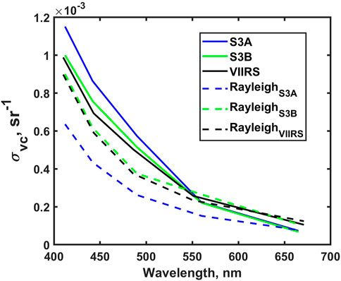
FIGURE 10. Standard deviations during system vicarious calibration for OLCI and VIIRS ${\sigma }_{vc}$ compared with Rayleigh component spectra for these sensors at the MOBY site.

5 Conclusion

Uncertainties in remote sensing reflectance for S3A and S3B OLCI sensors were evaluated by comparisons with MOBY and AERONET-OC data for several US and European sites. We applied a previously developed model for the decomposition of uncertainties spectra for OC satellite sensors to OLCI sensors and compared the results with the uncertainties from SNPP VIIRS. The uncertainties for OLCI and VIIRS are found to be spectrally similar, but at the coastal sites OLCI uncertainties are about 50% higher.

It is shown that as previously for VIIRS, the main component in $R_{rs}$ uncertainties spectra from OLCI is the Rayleigh component. For coastal water areas, the water variability term proportional to $R_{rs}$ spectra is also pronounced. All other components like aerosol, surface and glint effects are much smaller. Since the spectra of uncertainties from aerosols are not known, it is possible that the contribution of these uncertainties is underestimated. The effect of absorbing aerosols can be more visible in biases, but their spectral dependence is small at the sites considered here.

As in Gilerson et al., 2022 it is assumed that uncertainties in the Rayleigh component are mostly associated with the variability of the atmospheric parameters (ROT) or with their estimation in the current atmospheric correction algorithms (inaccuracies in modeling of the surface pressure), and/or with variability in the vertical distribution of atmospheric gaseous components. This uncertainty corresponds to about 1.5% of ROT at the MOBY site and higher at other stations. The Rayleigh spectral component of the uncertainties was equal to the standard deviation of gains in the vicarious calibration process after conversion to $R_{rs}$ uncertainties and is close to similar terms for other OC sensors. The reasons for some small differences remain unclear because of the differences in the standard deviations of the spectra of gains for OLCI S3A and S3B. Rayleigh-type uncertainties appear to be the main reason for the negative $R_{rs}$ values in coastal waters, where $R_{rs}$ themselves are typically small. Positive uncertainties in coastal areas and all uncertainties in the open ocean create some inaccuracies in $R_{rs}$ retrievals, but they are not explicitly visible as errors at high $R_{rs}$.

The reason for the higher uncertainties of OLCI, primarily with Rayleigh spectral shape, in comparison with VIIRS should be further studied. They may be partially related to some specifics in the atmospheric correction processing. In a preliminary manner, we associate them here with the latitude of the site and thus with the solar zenith angle, where in previous studies (Zibordi et al., 2022) dependence on the viewing angle was also noticed. Such dependencies do not exist for the SNPP VIIRS sensor.

To mitigate Rayleigh-type uncertainties atmospheric correction schemes should probably include additional constraints (Steinmetz et al., 2011), which can be even different for open ocean and costal water areas.

Data availability statement

The raw data supporting the conclusion of this article will be made available by the authors, without undue reservation.

Author contributions

AG, EH-E, JA, and RF formulated the original concept of the model. JG, DD, and EK provided OLCI data, described their features and uncertainties. EH-E processed satellite and AERONET-OC data. All authors participated in the uncertainty analysis from different components and provided critical feedback to the final manuscript. All authors contributed to the article and approved the submitted version.

Funding

The funding of this study was provided by the NOAA JPSS Cal/Val and JPSS PGRR programs, CESSRST Grant, NA16SEC4810008, and the NASA OBB grant, 80NSSC21K0562.

Acknowledgments

We thank NASA OBPG for the VIIRS satellite imagery, NASA AERONET Group for processing of the satellite data and support of the operation at the LISCO site. We are grateful to Kenneth Voss and the MOBY team for the MOBY data, PIs of AERONET-OC sites: Giuseppe Zibordi (Venise, Gloria, HLT), Marco Talone and Frederic Melin from the Joint Research Centre (JRC) of the European Commission (Casablanca), Robert Arnone, Alan Wiedemann, Bill Gibson and Sherwin Ladner (WaveCIS), Burton Jones and Matthew Ragan (USC). We also thank the Graduate Center of the City University of New York, The City College of New York, NOAA Center for Earth System Sciences and Remote Sensing Technologies, and NOAA Office of Education, Educational Partnership Program for fellowship support for Eder Herrera Estrella. The statements contained within the research article are not the opinions of the funding agency or the U.S. government but reflect the authors’ opinions. We are grateful to two reviewers whose recommendations led to the improvement of the manuscript.

Conflict of interest

The authors declare that the research was conducted in the absence of any commercial or financial relationships that could be construed as a potential conflict of interest.

Publisher’s note

All claims expressed in this article are solely those of the authors and do not necessarily represent those of their affiliated organizations, or those of the publisher, the editors and the reviewers. Any product that may be evaluated in this article, or claim that may be made by its manufacturer, is not guaranteed or endorsed by the publisher.

References

Ahmad, Z., Franz, B. A., McClain, C. R., Kwiatkowska, E., Werdell, J., Shettle, E. P., et al. (2010). New aerosol models for the retrieval of aerosol optical thickness and normalized water-leaving radiances from the SeaWiFS and MODIS sensors over coastal regions and open oceans. Appl. Opt. 49, 5545. doi:10.1364/AO.49.005545

PubMed Abstract | CrossRef Full Text | Google Scholar

Bailey, S. W., Franz, B. A., and Werdell, P. J. (2010). Estimation of near-infrared water-leaving reflectance for satellite ocean color data processing. Opt. Express 18, 7521–7527. doi:10.1364/OE.18.007521

PubMed Abstract | CrossRef Full Text | Google Scholar

Brown, S. W., Flora, S. J., Feinholz, M. E., Yarbrough, M. A., Houlihan, T., Peters, D., et al. (2007). “The marine optical buoy (MOBY) radiometric calibration and uncertainty budget for ocean color satellite sensor vicarious calibration,” in Proceedings of SPIE - The International Society for Optical Engineering, 6744. doi:10.1117/12.737400

CrossRef Full Text | Google Scholar

Clark, D. K., Gordon, H. R., Voss, K. J., Ge, Y., Broenkow, W., and Trees, C. C. (1997). Validation of atmospheric correction over the oceans. J. Geophys. Res. 102, 17209–17217. doi:10.1029/96JD03345

CrossRef Full Text | Google Scholar

Coleman, T. F., and Li, Y. (1994). On the convergence of interior-reflective Newton methods for nonlinear minimization subject to bounds. Math. Program. 67 (2), 189–224. doi:10.1007/BF01582221

CrossRef Full Text | Google Scholar

Coleman, T. F., and Li, Y. (1996). An interior, trust region approach for nonlinear minimization subject to bounds. SIAM J. Optim. 6 (2), 418–445. doi:10.1137/0806023

CrossRef Full Text | Google Scholar

Cox, C., and Munk, W. (1954). Measurement of the roughness of the sea surface from photographs of the sun’s glitter. J. Opt. Soc. Am. 44 (11), 838–850. doi:10.1364/JOSA.44.000838

CrossRef Full Text | Google Scholar

El-Habashi, A., Ahmed, S., Ondrusek, M., and Lovko, V. (2019). Analyses of satellite ocean color retrievals show advantage of neural network approaches and algorithms that avoid deep blue bands. J. Appl. Rem. Sens. 13 (2), 1. doi:10.1117/1.JRS.13.024509

CrossRef Full Text | Google Scholar

EUMETSAT (2020). Ocean Colour system vicarious calibration tool. Available at: https://www.eumetsat.int/ocean-colour-system-vicarious-calibration-tool (Accessed December 22, 2022).

Google Scholar

EUMETSAT. (2021). Sentinel-3 OLCI L2 Report for baseline collection Ol_l2m_003. Available at: https://www.eumetsat.int/media/47794 (Accessed December 20, 2022).

Google Scholar

EUMETSAT (2022). Recommendations for sentinel-3 OLCI Ocean Colour product validations in comparison with in situ measurements – matchup protocols. Available at: https://www.eumetsat.int/media/44087 (Accessed December 20, 2022).

Google Scholar

Fan, Y., Li, W., Chen, N., Ahn, J-H., Park, Y-J., Kratzer, S., et al. (2021). OC-SMART: A machine learning based data analysis platform for satellite ocean color sensors. Remote Sens. Environ. 253, 112236. doi:10.1016/j.rse.2020.112236

CrossRef Full Text | Google Scholar

Fougnie, B., Marbach, T., Lacan, A., Lang, R., Shlussel, P., Poli, G., et al. (2018). The multi-viewing multi-channel multi-polarisation imager – overview of the 3MI polarimetric mission for aerosol and cloud characterization. J. Quant. Spectrosc. Radiat. Transf. 219, 23–32. doi:10.1016/j.jqsrt.2018.07.008

CrossRef Full Text | Google Scholar

Franz, B. A., Bailey, S. W., Werdell, P. J., and McClain, C. R. (2007). Sensor-independent approach to the vicarious calibration of satellite ocean color radiometry. Appl. Opt. 46, 5068. doi:10.1364/AO.46.005068

PubMed Abstract | CrossRef Full Text | Google Scholar

Frouin, R., Schwindling, M., and Deschamps, P. Y. (1996). Spectral reflectance of sea foam in the visible and near-infrared: In situ measurements and remote sensing implications. J. Geophys. Res. Ocean. 101 (C6), 14361–14371. doi:10.1029/96JC00629

CrossRef Full Text | Google Scholar

Frouin, R. J., Franz, B. A., Ibrahim, A., Knobelspiesse, K., Ahmad, Z., Cairns, B., et al. (2019). Atmospheric correction of satellite ocean-color imagery during the PACE era. Front. Earth Sci. 7–145. doi:10.3389/feart.2019.00145

CrossRef Full Text | Google Scholar

Gao, M., Knobelspiesse, K., Franz, B. A., Zhai, P.-W., Sayer, A. M., Ibrahim, A., et al. (2022). Effective uncertainty quantification for multi-angle polarimetric aerosol remote sensing over ocean, Atmos. Meas. Tech., 15, 4859–4879. doi:10.5194/amt-15-4859-2022

CrossRef Full Text | Google Scholar

Gergely, M., and Zibordi, G. (2014). Assessment of AERONET-OC LWN uncertainties. Metrologia 51 (1), 40–47. doi:10.1088/0026-1394/51/1/40

CrossRef Full Text | Google Scholar

Gilerson, A., Malinowski, M., Herrera, E., Tomlinson, M., Stumpf, R., and Ondrusek, M. (2021). “Estimation of chlorophyll-a concentration in complex coastal waters from satellite imagery,” in Proceedings of SPIE 11752, Ocean Sensing and Monitoring XIII. doi:10.1117/12.2588004

CrossRef Full Text | Google Scholar

Gilerson, A., Herrera-Estrella, E., Foster, R., Agagliate, J., Hu, C., Ibrahim, A., et al. (2022). Determining the primary sources of uncertainty in retrieval of marine remote sensing reflectance from satellite Ocean Color sensors. Front. Remote Sens. 3. doi:10.3389/frsen.2022.857530

CrossRef Full Text | Google Scholar

Gordon, H. R., and Morel, A. Y. (1983). “In-water algorithms,” in Remote assessment of ocean color for interpretation of satellite visible imagery: A review. Editors H. R. Gordon, and A. Y. Morel (Berlin, Germany: Springer-Verlag). doi:10.1007/978-1-4684-6280-7,

CrossRef Full Text | Google Scholar

Gordon, H. R., and Wang, M. (1992). Surface-roughness considerations for atmospheric correction of ocean color sensors 1: The Rayleigh-scattering component. Appl. Opt. 31 (21), 4247–4260. doi:10.1364/AO.31.004247

PubMed Abstract | CrossRef Full Text | Google Scholar

Gordon, H. R., and Wang, M. (1994). Retrieval of water-leaving radiance and aerosol optical thickness over the oceans with SeaWiFS: A preliminary algorithm. Appl. Opt. 3, 443–452. doi:10.1364/ao.33.000443

PubMed Abstract | CrossRef Full Text | Google Scholar

Gordon, H. R., Du, T., and Zhang, T. (1997). Remote sensing of ocean color and aerosol properties: Resolving the issue of aerosol absorption. Appl. Opt. 36, 8670. doi:10.1364/AO.36.008670

PubMed Abstract | CrossRef Full Text | Google Scholar

Herrera-Estrella, E., Gilerson, A., Foster, R., and Groetsch, P. (2021). Spectral decomposition of remote sensing reflectance variance due to the spatial variability from ocean color and high-resolution satellite sensors. J. Appl. Rem. Sens. 15 (2), 024522. doi:10.1117/1.JRS.15.024522

CrossRef Full Text | Google Scholar

Hieronymi, M., Müller, D., and Doerffer, R. (2017). The OLCI neural network swarm (ONNS): A bio-geo-optical algorithm for open Ocean and coastal waters. Front. Mar. Sci. 4, 140. doi:10.3389/fmars.2017.00140

CrossRef Full Text | Google Scholar

Hlaing, S., Harmel, T., Gilerson, A., Foster, R., Weidemann, A., Arnone, R., et al. (2013). Evaluation of the VIIRS ocean color monitoring performance in coastal regions. Remote Sens. Environ. 139, 398–414. doi:10.1016/j.rse.2013.08.013

CrossRef Full Text | Google Scholar

IOCCG (2008). “Why ocean colour? The societal benefits of ocean-colour technology,” in Report No. 7 of the international ocean-colour coordinating group. Editors T. Platt, N. Hoepffner, V. Stuart, and C. Brown (Dartmouth, NS: IOCCG). doi:10.25607/OBP-97)

CrossRef Full Text | Google Scholar

IOCCG (2010). “Atmospheric correction for remotely-sensed ocean-colour products,” in Reports No. 10 of the international ocean-colour coordinating group. Editor M. Wang (Dartmouth, NS: IOCCG).

Google Scholar

IOCCG (2019). “Uncertainties in Ocean Colour remote sensing,” in Reports No. 18 of the international ocean-colour coordinating group. Editor F. Mélin (Dartmouth, NS: IOCCG). doi:10.25607/OBP-696:

CrossRef Full Text | Google Scholar

IOCCG (2021). “Observation of harmful algal blooms with Ocean Colour radiometry,” in Reports No. 20 of the international ocean-colour coordinating group. Editors S. Bernard, R. Kudela, L. Robertson Lain, and G. C. Pitcher (Dartmouth, NS: IOCCG). doi:10.25607/OBP-1042

CrossRef Full Text | Google Scholar

Melin, F. (2022). Validation of ocean color remote sensing reflectance data: Analysis of results at European coastal sites. Remote Sens. Environ. 280, 113153. doi:10.1016/j.rse.2022.113153

CrossRef Full Text | Google Scholar

Mikelsons, K., Wang, M., Kwiatkowska, E., Jiang, L., Dessailly, D., and Gossn, J. I. (2022). Statistical evaluation of sentinel-3 OLCI Ocean Color data retrievals. IEEE Trans. Geoscience Remote Sens. 60, 1–19. doi:10.1109/TGRS.2022.3226158

CrossRef Full Text | Google Scholar

C. D. Mobley (Editor) (2022). The oceanic optics book (Dartmouth, NS, Canada: International Ocean Colour Coordinating Group). doi:10.25607/OBP-1710

CrossRef Full Text | Google Scholar

Moore, T. S., Campbell, J. W., and Feng, H. (2015). Characterizing the uncertainties in spectral remote sensing reflectance for SeaWiFS and MODIS-Aqua based on global in situ matchup data sets. Remote Sens. Environ. 159, 14–27. doi:10.1016/j.rse.2014.11.025

CrossRef Full Text | Google Scholar

Morel, A., Antoine, D., and Gentili, B. (2002). Bidirectional reflectance of oceanic waters: Accounting for Raman emission and varying particle scattering phase function. Appl. Opt. 41 (30), 6289–6306. doi:10.1364/AO.41.006289

PubMed Abstract | CrossRef Full Text | Google Scholar

Oo, M., Vargas, M., Gilerson, A., Gross, B., Moshary, F., and Ahmed, S. (2008). Improving atmospheric correction for highly productive coastal waters using the short wave infrared retrieval algorithm with water-leaving reflectance constraints at 412 nm. Appl. Opt. 47 (21), 3846–3859. doi:10.1364/AO.47.003846

PubMed Abstract | CrossRef Full Text | Google Scholar

Qi, L., Lee, Z., Hu, C., and Wang, M. (2017). Requirement of minimal signal-to-noise ratios of ocean color sensors and uncertainties of ocean color products. J. Geophys. Res. Oceans 122 (3), 2595–2611. doi:10.1002/2016JC012558

CrossRef Full Text | Google Scholar

Ransibrahmanakul, V., and Stumpf, R. P. (2006). Correcting ocean colour reflectance for absorbing aerosols. Int. J. Remote Sens. 27 (9), 1759–1774. doi:10.1080/01431160500380604

CrossRef Full Text | Google Scholar

S3 OLCI Cyclic Performance Report (2021). Sentinel 3 mission performance center. Available at: https://sentinels.copernicus.eu/documents/247904/4602602/Sentinel-3-MPC-ACR-OLCI-Cyclic-Report-076-057.pdf (Accessed March 3, 2023).

Google Scholar

Shi, W., and Wang, M. (2007). Detection of turbid waters and absorbing aerosols for the MODIS ocean color data processing. Rem. Sens. Environm. 110 (2): 149–161. doi:10.1016/j.rse.2007.02.013

CrossRef Full Text | Google Scholar

Siegel, D. A., Wang, M., Maritorena, S., and Robinson, W. (2000). Atmospheric correction of satellite ocean color imagery: The black pixel assumption. Appl. Opt. 39 (21), 3582–3591. doi:10.1364/AO.39.003582

PubMed Abstract | CrossRef Full Text | Google Scholar

Steinmetz, F., Deschamps, P. Y., and Ramon, D. (2011). Atmospheric correction in presence of sun glint: Application to MERIS. Opt. Express 19 (10), 9783–9800. doi:10.1364/OE.19.009783

PubMed Abstract | CrossRef Full Text | Google Scholar

Tynes, H. H., Kattawar, G. W., Zege, E. P., KatsevPrikhach, I. L. A. S., and Chaikovskaya, L. I. (2001). Monte Carlo and multicomponent approximation methods for vector radiative transfer by use of effective Mueller matrix calculations. Appl. Opt. 40 (3), 400–412. doi:10.1364/AO.40.000400

PubMed Abstract | CrossRef Full Text | Google Scholar

Voss, K. J., Gordon, H. R., Flora, S., Johnson, B. C., Yarbrough, M., Feinholz, M., et al. (2017). A method to extrapolate the diffuse upwelling radiance attenuation coefficient to the surface as applied to the Marine Optical Buoy (MOBY). J. Atmos. Ocean. Technol. 34 (7), 1423–1432. doi:10.1175/JTECH-D-16-0235.1

PubMed Abstract | CrossRef Full Text | Google Scholar

Wang, M., and Bailey, S. W. (2001). Correction of sun glint contamination on the SeaWiFS ocean and atmosphere products. Appl. Opt. 40 (27), 4790–4798. doi:10.1364/AO.40.004790

PubMed Abstract | CrossRef Full Text | Google Scholar

Wang, M. (2007). Remote sensing of the ocean contributions from ultraviolet to near-infrared using the shortwave infrared bands: Simulations. Appl. Opt. 46, 1535–1547. doi:10.1364/AO.46.001535

PubMed Abstract | CrossRef Full Text | Google Scholar

Werdell, P. J., Behrenfeld, M. J., Bontempi, P. S., Boss, E., Cairns, B., Davis, G. T., et al. (2019). The Plankton, aerosol, cloud, ocean Ecosystem mission: Status, science, advances. Bull. Am. Meteorol. Soc. 100 (9), 1775–1794. doi:10.1175/BAMS-D-18-0056.1

CrossRef Full Text | Google Scholar

Xiong, X., Angal, A., Chang, T., Chiang, K., Lei, N., Li, Y., et al. (2020). MODIS and VIIRS calibration and characterization in support of producing long-term high-quality data products. Rem. Sens. 12 (19), 3167. doi:10.3390/rs12193167

CrossRef Full Text | Google Scholar

Zhang, M., Hu, C., and Barnes, B. B. (2019). Performance of POLYMER atmospheric correction of Ocean Color imagery in the presence of absorbing aerosols. IEEE Trans. Geosci. Remote. Sens. 57 (9), 6666–6674. doi:10.1109/TGRS.2019.2907884

CrossRef Full Text | Google Scholar

Zibordi, G., Mélin, F., Berthon, J. F., Holben, B., Slutsker, I., Giles, D., et al. (2009). AERONET-OC: A network for the validation of Ocean Color primary products. J. Atmos. Ocean. Technol. 26 (8), 1634–1651. doi:10.1175/2009JTECHO654.1

CrossRef Full Text | Google Scholar

Zibordi, G., Holben, B. N., Talone, M., D’Alimonte, D., Slutsker, I., Giles, D. M., et al. (2021). Advances in the Ocean Color component of the aerosol robotic network (AERONET-OC). Ocean. Technol. 38 (4), 725–746. doi:10.1175/JTECH-D-20-0085.1

CrossRef Full Text | Google Scholar

Zibordi, G., Kwiatkowska, E., Melin, F., Talone, M., Cazzaniga, I., Dessailly, D., et al. (2022). Assessment of OLCI-A and OLCI-B radiometric data products across European seas. Remote. Sens. Environ. 272, 112911. doi:10.1016/j.rse.2022.112911

CrossRef Full Text | Google Scholar