Corrigendum: An operational approach to near real time global high resolution mapping of the terrestrial human footprint
 Francis Gassert1Oscar Venter2
 James E. M. Watson3,4Steven P. Brumby5
 Joseph C. Mazzariello5*†
 Scott C. Atkinson3,6Samantha Hyde5
- 1Vizzuality, Madrid, Spain
- 2Natural Resource and Environmental Studies Institute, University of Northern British Columbia, Prince George, BC, Canada
- 3School of Earth and Environmental Sciences, University of Queensland, Brisbane, QLD, Australia
- 4Centre for Biodiversity and Conservation Science, University of Queensland, Brisbane, QLD, Australia
- 5Impact Observatory, Washington, DC, United States
- 6United Nations Development Programme, New York, NY, United States
Introduction
Over the past two decades the mapping of human pressures has become a critical tool for scientific research and policy making (Watson and Venter, 2019). Human pressures, or lack thereof, are associated with habitat loss (Riggio et al., 2020; Verma et al., 2020), deforestation and degradation risk (Ordway et al., 2017), and species extinction risk (Di Marco et al., 2018; O’Bryan et al., 2020a; O’Bryan et al., 2020b). Human pressure maps have become an important tool for spatial planning (Tulloch et al., 2015) and land use management (Garnett et al., 2018), monitoring the extent of human influence (Venter et al., 2016a; Williams et al., 2020), and identifying critical remaining intact habitat (Watson et al., 2016a; Williams et al., 2020).
In this study we use the Human Footprint methodology first described by Sanderson and others in 2002 (Sanderson et al., 2002), to produce the first global 100 m resolution human pressure map time series. Human Footprint combines indicators of land cover, population, infrastructure, and accessibility to estimate the magnitude of human pressure (Sanderson et al., 2002). We take advantage of data layers from diverse sources to identify where humans exert influence on the terrestrial planet. By combining both top down and bottom up data sources, human pressure mapping is able to identify stresses that are difficult to identify using only remotely-sensed data, while providing wider and more consistent coverage than field-based approaches (Venter et al., 2016b; Watson and Venter, 2019).
This study builds off past work to map global Human Footprint (Sanderson et al., 2002; Venter et al., 2016b; Williams et al., 2020; Mu et al., 2022), and joins other global human pressure mapping efforts, including the Global Human Modification (gHM) index (Kennedy et al., 2019; Theobald et al., 2020), which estimates the extent to which land has been modified by human stressors; Low Impact Areas (LIA) (Jacobson et al., 2019) which identifies areas that are subject to minimal human pressure; and others (Geldman et al., 2014). Human Footprint differs from these approaches in several ways. Most notable is its inclusion of accessibility measures, which identify areas which may otherwise appear undisturbed but are easily exploitable. The Human Footprint also attempts a simpler and more transparent approach than the gHM, for example, which uses more input datasets and combines them with additional statistical techniques. Along those lines, the Human Footprint methodology focuses more on input variables that are higher spatial resolution (100 m vs. 1 km for gHM and LIA) and higher temporal resolution (i.e., annual cadance) that are also expected to continue being updated into the future for continued updates.
While many previous mapping efforts are trusted as geospatial products, governments still have a critical information gap in understanding recent and ongoing change (Watson and Venter, 2019). The software and methods described here are designed to be run on a continued basis into the future to enable regular updates to this critical dataset, including anticipated advances in remote sensing data. This approach is intended to address the shortfall in efforts around existing mapping outputs, which tend to be perpetually several years out of date when released. We also release a 100 m global gridded dataset for the years 2015–2019 and 2020 so as to provide the latest update.
Materials and methods
Experimental design
We follow the prior methods of Sanderson et al. (2002); Venter et al. (2016b); Williams et al. (2020) to create the Human Footprint maps. We use data on human pressures across the period 2015 to 2019 and for 2020 to map: 1) Land cover change (built environments, crop lands, and pasture lands), 2) population density, 3) electric infrastructure, 4) roadways, 5) railways, and 6) navigable waterways. Each pressure layer is assigned a score between 0 and 10 relative to its level of human pressure following Sanderson et al. (2002). We compute standardized Human Footprint maps on a scale of 0–501 as the sum of all pressure layers. Pressures are not mutually exclusive, rather the co-occurrence of pressures is intended to identify the greatest levels of human impact. The majority of layers cover the complete time period of 2015–2020, however pressures from pasture, roads, and railways are treated as static in the Human Footprint maps due to limitations in the input datasets. As of the time of writing of this paper, our methodology also benefits from two layers, the 10 m ESRI-LC and VIIRS Annual Night Time Lights v2, being consistently updated for future versions past 2020; other layers such as the OSM roads may also be updated for future versions, albeit perhaps infrequently and inconsistently around the globe.
These methods are implemented in scripts in the open source Python programming language, and are designed to run operationally on an annual basis to provide continued monitoring of changing anthropogenic pressures on the natural world. This includes two key design choices in its implementation. First, we innovate on the Human Footprint methodology by defining and implementing it in a manner agnostic to the source and scale of input data. Most pressure mapping efforts, including previous iterations of Human Footprint, measure the presence or absence of stresses at a given spatial resolution (Watson et al., 2016a; Watson et al., 2016b). In this study, layers that are not direct remote sensing observations are normalized using linear distance measures, such that results are consistent regardless of the spatial resolution of input datasets and desired output resolution. Second, variables are fully parameterized such that they can be easily updated or alternate data sources can be swapped in, pressure weightings, normalization scales, output scale and extent can be adjusted. This approach is developed to utilize continued advancements in remote sensing technology and accessibility of computational capabilities enabling more frequent, higher-resolution measurements.
The remainder of this section describes the methods and data used to produce the global 100 m Human Footprint maps for 2015–2019 as well as 2020. These data are computed in the Molleweide equal area projection, yielding ∼13.4 billion pixels covering Earth’s non-Antarctic terrestrial surface. Computation was performed using open source Python libraries in the Microsoft Planetary Computer infrastructure.
Land cover change
Land cover change pressures were mapped using a combination of three layers: Built environments, crop lands, and pasture lands. Built environments include buildings and paved areas, which make up the bulk of urban areas but may also appear in peri-urban and rural zones. Crop lands vary in their structure from intensely managed monocultures receiving high inputs of pesticides and fertilizers, to mosaic agricultures, such as slash and burn methods that can support intermediate levels of natural values (Luck and Daily, 2003; Fischer et al., 2008). Pasture lands grazed by domesticated herbivores are often degraded through a combination of fencing, intensive browsing, soil compaction, invasive grasses and other species, and altered fire regimes (Kauffman and Krueger, 1984).
We map both built environments and crop lands using the Copernicus Global Land Service Dynamic Land Cover Map at 100 m resolution version 3 (CGLS-LC100) (Buchhorn et al., 2020) for the years 2015–2019, and the ESRI 2020 Global Land Use Land Cover from Sentinel-2 (ESRI LC) for the year 2020. CGLS-LC100 is produced following a supervised classification of imagery from the PROBA-V satellite. ESRI LC is produced using a machine learning approach based on 10 m imagery from the Sentinel-2 satellites.
In contrast to previous versions of human footprint which used nighttime lights (Elvidge et al., 2001; Baugh et al., 2010) to identify urban areas, the relatively high resolution of CGLS-LC100 is able to identify urban parks and corridors that may provide important habitat connectivity for terrestrial species, as well as isolated built environments outside of urban centers (Kattwinkel et al., 2011). Similarly, this layer is better able to resolve agricultural mosaics than previously used land cover maps (Herold et al., 2008), though may still be limited in mapping sparse and very small scale agriculture.
We map pasture lands using a spatial dataset that combines agricultural census data with satellite-derived land cover to estimate the percentage of land area that is used for pasture at a 1 km2 gridded resolution for the year 2000 (Ramankutty et al., 2008). While this is a static dataset, we updated it using the land use exclusion principle that urban, crops, and pasture cannot co-occur, and that these land uses exclude one another following the listed order. As the crop and urban layers are more recent and intended to be dynamic, they are used to derive a modified pasture layer for each year.
As built environments do not provide viable habitats for many species of conservation concern, nor do they provide high levels of ecosystem services (Tratalos et al., 2007; Aronson et al., 2014), they are assigned a pressure score of 10. Although intensive agriculture often results in whole-scale ecosystem conversion, we assign croplands a score of 7, lower than built areas due to them being less impervious. Pasture is assigned the lowest relative score of 4.
Population density
The intensity of human pressure on the environment is often associated with proximity to human populations, such as human disturbance, hunting, and the persecution of non-desired native species (Brashares et al., 2001). Even low-density human populations with limited development can have significant impacts on biodiversity (Burney and Flannery, 2005; Miller et al., 2005). We incorporated human population density using the WorldPop Unconstrained individual countries 2000–2020 100 m resolution dataset (WorldPop, 2020; Lloyd et al., 2019).
The dataset provides a 3 arcsecond (∼100 m2) gridded estimate of residential population count for all countries derived from recent census data and is dasymetrically distributed using satellite-derived covariates. We convert population counts to population density using a 1 km × 1 km square kernel. Locations with more than 1,000 people per km2 receive a maximum pressure score of 10. For more sparsely populated areas, we logarithmically scaled the pressure score using:
Population density is scored in this way under the assumption that the pressures people induce on their local natural systems increase logarithmically with increasing population density, and saturate at a level of 1,000 people km−2.
Nighttime lights
We use the VIIRS Annual Night Time Lights version 2 (VNL v2) dataset (Elvidge et al., 2021) as a means of mapping electric infrastructure. In addition to urban centers, rural and suburban areas illuminated at night are often representative of important human infrastructure, such as rural housing, working landscapes, and industrial installations, with associated pressures on natural environments (Small et al., 2011).
VNL v2 provides estimates of average annual radiance (µW/cm2/sr) at the 15 arc second (∼500 m) resolution, corrected for stray light sources and outliers. We assign a maximum score of 10 to a radiance of 25 μW/cm2/sr, a brightness typically exceeded in moderately-sized cities in developed countries (Levin and Zhang, 2017), and score values less than 25 on a logarithmic scale using:
Roads
As one of humanity’s most prolific linear infrastructures, roads are an important direct driver of habitat conversion (Trombulak and Frissell, 2000). Beyond simply reducing the extent of suitable habitat, roads can act as population sinks for many species through traffic-induced mortality (Woodroffe and Ginsberg, 1998). Roads also fragment otherwise contiguous blocks of habitat, and create edge effects, such as reduced humidity and increased fire frequency that reach well beyond the road’s immediate footprint (Adeney et al., 2009). Finally, roads provide conduits for humans to access nature, bringing hunters and nature users into otherwise largely natural and intact locations (Forman and Alexander, 1998).
Data from OpenStreetMap (OSM) on roads and railways is extracted from the global OSM planet database (Planet, 2021). OSM is a volunteer-driven, open access global mapping project that has grown enormously in spatial completeness since its inception in 2004. The volume and coverage of global transportation networks in the OSM database has far surpassed previously available roads data (e.g., gRoads) that was used in earlier iterations of the Human Footprint. However, as the OSM dataset does not provide true and comprehensive temporal information on road creation (as opposed to initial inclusion in the database), we treat it as a static dataset, using the most up-to-date data for the entire 2015–2020 period.
We map roads using linear features tagged “highway”, excluding minor features such as farm tracks, footways, and cycle paths, as well as tunnels, which may run under otherwise undisturbed natural areas. We map the direct and indirect influence of roads assigning a score of 8 to pixels within a 0.5 km buffer on either side of roads. We additionally map pressures associated with the access that roads provide (e.g., collection, extraction, and hunting) with a score of 4 at a distance of 1.0 km and decaying exponentially out to 15 km from either side of a road.
Railways
While railways are an important component of our global transport system, their pressure on the environment differs in nature from that of our road networks. By modifying a linear swath of habitat, railways exert direct pressure where they are constructed, similar to roads. However, as passengers seldom disembark from trains in places other than rail stations, railways do not provide a means of accessing the natural environments along their borders. The direct pressure of railways is assigned a score of 8 for a 0.5 km buffer on either side of the railway. We exclude railways tagged as abandoned, disused, and proposed as well as tunnels.
Navigable waterways
Like roads, coastlines and navigable rivers act as conduits for people to access nature. For the purposes of the Human Footprint we only consider coastlines and rivers to be navigable if they are within 80 km of signs of a human settlement, which are mapped as a nighttime lights signal with a radiance greater than 1 µW/cm2/sr that is also within 4 km of the coast or river bank. Coastlines are derived from HydroSHEDS (Lehner and Grill, 2013) ocean masks for regions less than 60° latitude, for all other regions we derived coastlines from the GTOPO30 ocean mask (USGS, 1997). We chose 80 km as an approximation of the distance a vessel can travel and return during daylight hours.
Rivers within 80 km of human settlements are considered navigable if their depth is greater than 2 m. To map rivers and their depth we use the HydroRIVERS dataset on stream discharge (Lehner and Grill, 2013). We estimated depth from discharge assuming second-order parabola as channel shape using the following formula:
We also considered lakes along navigable rivers (typically reservoirs), as well as lakes with a surface area of at least 100 km2 and average depth of at least 3 m to be navigable coastlines. The largest of lakes can act essentially as inland seas, used extensively for trade, transit, and recreation. We map lakes using the complimentary HydroLAKES dataset (Messager et al., 2016).
As new settlements can arise to make waterways newly navigable, layers are created for each year (2015–2020). The access pressure from navigable waterways is assigned a score of 4 within 0.5 km of the water body, decaying exponentially out to 15 km.
Validation
We evaluate the performance of the Human Footprint maps against a validation dataset originally produced for the Venter et al. version of Human Footprint (Venter et al., 2016b). This dataset includes scores derived from expert interpretation of high resolution satellite imagery taken between 1999 and 2012 for 3,114 points randomly sampled from the land area of the globe. Plots were scored on a scale of 0–13 based on the extent of built environments, crop lands, pasture lands, roads, human settlements, infrastructures and navigable waterways following a standard key for identifying these features (Venter et al., 2016b Supplementary Material S1).
We extract the mean Human Footprint score from a 1 × 1 km2 square centered on each validation site, and normalize both validation scores and Human Footprint scores to a 0–1 scale for comparison. For the 2020 Human Footprint based on the 10 m ESRI-LC we find a root mean square error of 0.105 indicating an average error of roughly 11%, and a Pearson’s correlation coefficient of 0.66 (Supplementary Table S3). For the 2019 Human Footprint based on the CGLS-LC100 land cover, we find similar levels of agreement with a root mean square error of 0.107.
These measures of agreement are conservative estimates of the map’s accuracy, as the nine to 20 year discrepancy between the 2020 Human Footprint map and global validation data would induce some error that is due only to true changes in human pressures. Despite this time discrepancy, results show improvement in validation statistics when compared to previous versions of Human Footprint.
We also validate 2020 Human Footprint scores against a more contemporaneous validation set for 4,674 sites randomly sampled from the land area of Canada (Hirsh-Pearson, 2020), and find a root mean square error of 0.136. Lower agreement levels reflect the explicit inclusion of oil, gas, mining, and forestry activities in the Canada validation dataset that are not measured at the global scale.
Analysis
Global 100 m Human Footprint maps are produced for 2015–2019 and 2020 (Figure 1). We find a global area average Human Footprint score for 2020 of 4.56, with 44% of land area with a score ≤1 “wilderness,” 21% with a score of 1–4 “low disturbance,” and 35% with a score >4 “highly modified” (Supplementary Table S1). The change between 2015 and 2019 shows an average increase in Human Footprint across the world of about 0.10 (out of 50), and a net change of 24 million hectares from “wilderness” to “low disturbance” and 33 million hectares from “low disturbance” to “highly modified.” Increases in Human Footprint appear the most pronounced in Tropical Forest, Mangrove, and Temperate Broadleaf Forest biomes (Supplementary Table S1). Because results for 2015–2019 and 2020 are generated using two different land cover datasets as inputs, comparisons between these two periods should be made with caution.
FIGURE 1
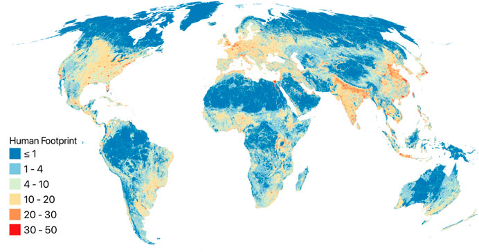
FIGURE 1. Global terrestrial Human Footprint for 2020.
Data availability statement
Publicly available datasets were analyzed in this study. This data can be found here: Files for the 2015-2019 and 2020 100m Human Footprint maps are available on the Dryad repository at: https://doi.org/10.5061/dryad.ttdz08m1f. Scripts used to produce this data are available at: https://gitlab.com/impactobservatory/dwi-humanfootprint.
Author contributions
Conceptualization: SB, OV, and JW. Methodology: FG, OV, JW, and SA. Software: FG and SA. Data curation: FG, SA, and JM. Visualization: FG. Supervision: SB and SH. Writing–original draft: FG, OV, and JW. Writing–review and editing: SH, OV, JW, and SA. All authors contributed to the article and approved the submitted version.
Funding
The authors declare that this study received funding from Microsoft. The funder was not involved in the study design, collection, analysis, interpretation of data, the writing of this article, or the decision to submit it for publication.
Conflict of interest
Author FG was employed by Vizzuality. Authors SB, JM, and SH were employed by Impact Observatory.
The remaining authors declare that the research was conducted in the absence of any commercial or financial relationships that could be construed as a potential conflict of interest.
Publisher’s note
All claims expressed in this article are solely those of the authors and do not necessarily represent those of their affiliated organizations, or those of the publisher, the editors and the reviewers. Any product that may be evaluated in this article, or claim that may be made by its manufacturer, is not guaranteed or endorsed by the publisher.
Supplementary material
The Supplementary Material for this article can be found online at: https://www.frontiersin.org/articles/10.3389/frsen.2023.1130896/full#supplementary-material
Footnotes
1We utilize a score of 0–50, as opposed to 0–60, purely to stay consistent with previous versions of HFP.
References
Adeney, J., Christensen, N., and Pimm, S. (2009). Reserves protect against deforestation fires in the amazon. PLOS ONE 4, e5014. doi:10.1371/journal.pone.0005014
Aronson, M., La Sorte, F., Nilon, C., Katti, M., Goddard, M., Lepczyk, C., et al. (2014). A global analysis of the impacts of urbanization on bird and plant diversity reveals key anthropogenic drivers. Proc. R. Soc. B Biol. Sci. 281, 20133330. doi:10.1098/rspb.2013.3330
Baugh, K., Elvidge, C., Ghosh, T., and Ziskin, D. (2010). Development of a 2009 stable lights product using DMSP-OLS data. Proc. Asia-Pac. Adv. Netw. 30, 114. doi:10.7125/APAN.30.17
Brashares, J., Arcese, P., and Sam, M. (2001). Human demography and reserve size predict wildlife extinction in West Africa. Proc. R. Soc. Lond. B Biol. Sci. 268, 2473–2478. doi:10.1098/rspb.2001.1815
Buchhorn, M., Bertels, L., Smets, B., Roo, B., Lesiv, M., Tsendbazar, N., et al. (2020). Copernicus global land service: land cover 100m: version 3 globe 2015-2019: algorithm theoretical basis document. Zenodo. doi:10.5281/zenodo.3938968
Burney, D., and Flannery, T. (2005). Fifty millennia of catastrophic extinctions after human contact. Trends Ecol. Evol. 20, 395–401. doi:10.1016/j.tree.2005.04.022
Di Marco, M., Venter, O., Possingham, H., and Watson, J. (2018). Changes in human footprint drive changes in species extinction risk. Nat. Commun. 9, 4621. doi:10.1038/s41467-018-07049-5
Elvidge, C., Imhoff, M., Baugh, K., Hobson, V., Nelson, I., Safran, J., et al. (2001). Night-time lights of the world: 1994–1995. ISPRS J. Photogramm. Remote Sens. 56, 81–99.
Elvidge, C., Zhizhin, M., Ghosh, T., Hsu, F., and Taneja, J. (2021). Annual time series of global VIIRS nighttime lights derived from monthly averages: 2012 to 2019. Remote Sens. 13. doi:10.3390/rs13050922
Fischer, J., Brosi, B., Daily, G., Ehrlich, P., Goldman, R., Goldstein, J., et al. (2008). Should agricultural policies encourage land sparing or wildlife-friendly farming? Front. Ecol. Environ. 6, 380–385. doi:10.1890/070019
Forman, R., and Alexander, L. (1998). Roads and their major ecological effects. Annu. Rev. Ecol. Syst. 29, 207–231.
Garnett, S. T., Burgess, N. D., Fa, J. E., Fernández-Llamazares, Á., Molnár, Z., Robinson, C. J., et al. (2018). A spatial overview of the global importance of Indigenous lands for conservation. Nat. Sustain. 1, 369–374. doi:10.1038/s41893-018-0100-6
Geldman, J., Joppa, L., and Burgess, N. (2014). Mapping change in human pressure globally on land and within protected areas. Conserv. Biol. 28, 1604–1616. doi:10.1111/cobi.12332
Herold, M., Mayaux, P., Woodcock, C., Baccini, A., and Schmullius, C. (2008). Some challenges in global land cover mapping: an assessment of agreement and accuracy in existing 1 km datasets. Earth Obs. Terr. Biodivers. Ecosyst. Spec. Issue. 112, 2538–2556. doi:10.1016/j.rse.2007.11.013
Hirsh-Pearson, K. (2020). “A framework for mapping cumulative threats and its application to Canada,”. thesis (Canada: University of Northern British Columbia).
Jacobson, A., Riggio, J., Tait, A., and Baillie, J. (2019). Global areas of low human impact (‘Low Impact Areas’) and fragmentation of the natural world. Sci. Rep. 9, 14179. doi:10.1038/s41598-019-50558-6
Kattwinkel, M., Biedermann, R., and Kleyer, M. (2011). Temporary conservation for urban biodiversity. Biol. Conserv. 144, 2335–2343. doi:10.1016/j.biocon.2011.06.012
Kauffman, J., and Krueger, W. (1984). Livestock impacts on riparian ecosystems and streamside management implications. A Rev. J. Range Manag. 37, 430–438. doi:10.2307/3899631
Kennedy, C., Oakleaf, J., Theobald, D., Baruch-Mordo, S., and Kiesecker, J. (2019). Managing the middle: a shift in conservation priorities based on the global human modification gradient. Glob. Change Biol. 25, 811–826. doi:10.1111/gcb.14549
Lehner, B., and Grill, G. (2013). Global river hydrography and network routing: baseline data and new approaches to study the world’s large river systems. Hydrol. Process. 27, 2171–2186. doi:10.1002/hyp.9740
Levin, N., and Zhang, Q. (2017). A global analysis of factors controlling VIIRS nighttime light levels from densely populated areas. Remote Sens. Environ. 190, 366–382.
Lloyd, C., Chamberlain, H., Kerr, D., Yetman, G., Pistolesi, L., Stevens, F., et al. (2019). Global spatio-temporally harmonised datasets for producing high-resolution gridded population distribution datasets. Big Earth Data 3, 108–139. doi:10.1080/20964471.2019.1625151
Luck, G., and Daily, G. (2003). Tropical Countryside Bird Assemblages: richness, Composition, And Foraging Differ By Landscape Context. Ecol. Appl. 13, 235–247. doi:10.1890/1051-0761(2003)013[0235:TCBARC]2.0.CO;2
Messager, M., Lehner, B., Grill, G., Nedeva, I., and Schmitt, O. (2016). Estimating the volume and age of water stored in global lakes using a geo-statistical approach. Nat. Commun. 7, 13603. doi:10.1038/ncomms13603
Miller, G., Fogel, M., Magee, J., Gagan, M., Clarke, S., and Johnson, B. (2005). Ecosystem collapse in pleistocene Australia and a human role in megafaunal extinction. Science 309, 287. doi:10.1126/science.1111288
Mu, H., Li, X., Wen, Y., Huang, J., Du, P., Su, W., et al. (2022). A global record of annual terrestrial Human Footprint dataset from 2000 to 2018. Sci. Data 9, 176. doi:10.1038/s41597-022-01284-8
O’Bryan, C., Allan, J., Holden, M., Sanderson, C., Venter, O., Di Marco, M., et al. (2020b). Intense human pressure is widespread across terrestrial vertebrate ranges. Glob. Ecol. Conserv. 21, e00882. doi:10.1016/j.gecco.2019.e00882
O’Bryan, C., Garnett, S., Fa, J., Leiper, I., Rehbein, J., Fernández-Llamazares, Á., et al. (2020a). The importance of Indigenous Peoples’ lands for the conservation of terrestrial mammals. Conserv. Biol. 2020. doi:10.1111/cobi.13620
Ordway, E., Asner, G., and Lambin, E. (2017). Deforestation risk due to commodity crop expansion in sub-Saharan Africa. Environ. Res. Lett. 12, 044015. doi:10.1088/1748-9326/aa6509
Planet (2021). OpenStreetMap contributors, Planet dump. Available at: https://planet.osm.org.
Ramankutty, N., Evan, A., Monfreda, C., and Foley, J. (2008). Farming the planet: 1. Geographic distribution of global agricultural lands in the year 2000. Glob. Biogeochem. Cycles. 22. doi:10.1029/2007GB002952
Riggio, J., Baillie, J., Brumby, S., Ellis, E., Kennedy, C., Oakleaf, J., et al. (2020). Global human influence maps reveal clear opportunities in conserving Earth’s remaining intact terrestrial ecosystems. Glob. Change Biol. 26, 4344–4356. doi:10.1111/gcb.15109
Sanderson, E., Jaiteh, M., Levy, M., Redford, K., Wannebo, A., and Woolmer, G. (2002). The Human Footprint and the Last of the Wild: the human footprint is a global map of human influence on the land surface, which suggests that human beings are stewards of nature, whether we like it or not. BioScience 52, 891–904. doi:10.1641/0006-3568(2002)052[0891:THFATL]2.0.CO;2
Small, C., Elvidge, C., Balk, D., and Montgomery, M. (2011). Spatial scaling of stable night lights. Remote Sens. Environ. 115, 269–280. doi:10.1016/j.rse.2010.08.021
Theobald, D., Kennedy, C., Chen, B., Oakleaf, J., Baruch-Mordo, S., and Kiesecker, J. (2020). Earth transformed: detailed mapping of global human modification from 1990 to 2017. Earth Syst. Sci. Data. 12, 1953–1972. doi:10.5194/essd-12-1953-2020
Tratalos, J., Fuller, R., Warren, P., Davies, R. G., and Gaston, K. (2007). Urban form, biodiversity potential and ecosystem services. Landsc. Urban Plan. 83, 308–317. doi:10.1016/j.landurbplan.2007.05.003
Trombulak, S., and Frissell, C. (2000). Review of ecological effects of roads on terrestrial and aquatic communities. Conserv. Biol. 14, 18–30. doi:10.1046/j.1523-1739.2000.99084.x
Tulloch, V., Tulloch, A., Visconti, P., Halpern, B., Watson, J., Evans, M., et al. (2015). Why do we map threats? Linking threat mapping with actions to make better conservation decisions. Front. Ecol. Environ. 13, 91–99. doi:10.1890/140022
USGS (1997). Global 30 arc-second elevation (GTOPO30). Available at: https://www.usgs.gov/centers/eros/science/usgs-eros-archive-digital-elevation-global-30-arc-second-elevation-gtopo30?qt-science_center_objects=0#overview (Accessed July 1, 2020). doi:10.5066/F7DF6PQS
Venter, O., Sanderson, E., Magrach, A., Allan, J., Beher, J., Jones, K., et al. (2016b). Global terrestrial human footprint maps for 1993 and 2009. Sci. Data. 3, 160067. doi:10.1038/sdata.2016.67
Venter, O., Sanderson, E. W., Magrach, A., Allan, J., Beher, J., Jones, K., et al. (2016a). Sixteen years of change in the global terrestrial human footprint and implications for biodiversity conservation. Nat. Commun. 7, 12558. doi:10.1038/ncomms12558
Verma, M., Symes, W., Watson, J., Jones, K., Allan, J., Venter, O., et al. (2020). Severe human pressures in the Sundaland biodiversity hotspot. Conserv. Sci. Pract. 2, e169. doi:10.1111/csp2.169
Watson, J., Jones, K., Fuller, R., Marco, M., Segan, D., Butchart, S., et al. (2016b). Persistent disparities between recent rates of habitat conversion and protection and implications for future global conservation targets. Conserv. Lett. 9, 413–421. doi:10.1111/conl.12295
Watson, J., Shanahan, D., Di Marco, M., Allan, J., Laurance, W. F., Sanderson, E. W., et al. (2016a). Catastrophic declines in wilderness areas undermine global environment targets. Curr. Biol. 26, 2929–2934. doi:10.1016/j.cub.2016.08.049
Watson, J., and Venter, O. (2019). Mapping the continuum of humanity’s footprint on land. One Earth 1, 175–180. doi:10.1016/j.oneear.2019.09.004
Williams, B. A., Venter, O., Allan, J. R., Atkinson, S. C., Rehbein, J. A., Ward, M., et al. (2020). Change in terrestrial human footprint drives continued loss of intact ecosystems. One Earth 3, 371–382. doi:10.1016/j.oneear.2020.08.009
Woodroffe, R., and Ginsberg, J. (1998). Edge effects and the extinction of populations inside protected areas. Science 280, 2126. doi:10.1126/science.280.5372.2126
WorldPop (2020). Population density: unconstrained individual countries 2000-2020 (1 km resolution). From: School of geography and environmental science, university of southampton; department of geography and geosciences, university of Louisville; departement de Geographie, universite de Namur), center for international Earth science information network (CIESIN), global high resolution population denominators project—funded by the bill and melinda gates foundation (OPP1134076). Available at: https://hub.worldpop.org/doi/10.5258/SOTON/WP00674 (Accessed Jul 1, 2020). doi:10.5258/SOTON/WP00674
Keywords: human footprint (HF), remote sensing, land use land cover (LULC), human impact, environmental impact
Citation: Gassert F, Venter O, Watson JEM, Brumby SP, Mazzariello JC, Atkinson SC and Hyde S (2023) An operational approach to near real time global high resolution mapping of the terrestrial Human Footprint. Front. Remote Sens. 4:1130896. doi: 10.3389/frsen.2023.1130896
Received: 23 December 2022; Accepted: 11 October 2023;
Published: 27 November 2023.
Edited by:
Yansheng Li, Wuhan University, ChinaReviewed by:
Kwame Oppong Hackman, West African Science Service Centre on Climate Change and Adapted Land Use (WASCAL), Burkina FasoR. Travis Belote, The Wilderness Society, Bozeman, MT, United States
Copyright © 2023 Gassert, Venter, Watson, Brumby, Mazzariello, Atkinson and Hyde. This is an open-access article distributed under the terms of the Creative Commons Attribution License (CC BY). The use, distribution or reproduction in other forums is permitted, provided the original author(s) and the copyright owner(s) are credited and that the original publication in this journal is cited, in accordance with accepted academic practice. No use, distribution or reproduction is permitted which does not comply with these terms.
*Correspondence: Joseph C. Mazzariello, joe@impactobservatory.com
†ORCID: Joseph C. Mazzariello, https://orcid.org/0000-0001-9888-8746