
95% of researchers rate our articles as excellent or good
Learn more about the work of our research integrity team to safeguard the quality of each article we publish.
Find out more
ORIGINAL RESEARCH article
Front. Remote Sens. , 01 September 2023
Sec. Image Analysis and Classification
Volume 4 - 2023 | https://doi.org/10.3389/frsen.2023.1123254
This article is part of the Research Topic Women in Remote Sensing: 2022 View all 16 articles
 Andressa Garcia Fontana1*
 Victor Fernandez Nascimento2
 Jean Pierre Ometto3
 Francisco Hélter Fernandes do Amaral4
This research investigates Land Use and Land Cover (LULC) changes in the Porto Alegre Metropolitan Region (RMPA). A 30-year historical analysis using Landsat satellite imagery was made and used to develop LULC scenarios for the next 20 years using a Multilayer Perceptrons (MLP) model through an Artificial Neural Network (ANN). These maps analyze the urban area’s expansion over the years and project their potential development in the future. This research considered several critical factors influencing urban growth, including shaded relief, slope, distances from main roadways, railway stations, urban centers, and the state capital, Porto Alegre. These spatial variables were incorporated into the model’s learning processes to generate future urbanization scenarios. The LULC historical maps precision showed excellent performance with a Kappa index greater than 88% for the studied years. The results indicate that the urbanization class witnessed an increase of 236.78 km2 between 1990 and 2020. Additionally, it was observed that the primary concentration of urbanized areas since 1990 has predominantly occurred around Porto Alegre and Canoas. Lastly, the future forecasts for LULC changes in 2030 and 2040 indicate that the urban area of the RMPA is projected to reach 1,137.48 km2 and 1,283.62 km2, respectively. In conclusion, based on the observed urban perimeter in 2020, future projections indicate that urban areas are expected to increase by more than 443.29 km2 by 2040. The combination of remote sensing data and Geographic Information System (GIS) enables the monitoring and modeling the metropolitan area expansion. The findings provide valuable insights for policymakers to develop more informed and conscientious urban plans, as well as enhance management techniques for urban development.
Changes in land use and land cover (LULC) are related to human activity, which tends to reside in cities in search of jobs, educational opportunities and access to better health services. Thus, due to economic growth, urbanization increases rapidly. Loss of natural areas and global climate change are just a few examples of environmental problems caused by LULC changes (Meraj et al., 2022). The transitions in built-up areas expansion could significantly impact the population’s quality of life (Ashaolu et al., 2019). Therefore, it is crucial to conduct urban expansion simulations.
There are various models available to simulate future scenarios, including regression models (Hu and Lo, 2007), cellular automata (Chen et al., 2016), and Markov chain models (Arsanjani et al., 2011), among others. The advancement of computational technology has enabled the integration of machine learning algorithms into studies involving cellular automata (CA) models. Algorithms such as Artificial Neural Network (ANN) (Li and Yeh, 2002), Support Vector Machine (SVM) (Yang et al., 2008), and Genetic Algorithm (GA) (Li et al., 2013) have been utilized to tackle challenges associated with parameter optimization in CA models. These methods optimize the model parameters to achieve the best possible results, effectively addressing simulation challenges related to multiple spatial variables.
However, there are different CA Models variants created to simulate urban sprawl change, such as SLEUTH (Clarke et al., 1997), the dynamic urban evolution model (Batty, 1997), the multicriteria decision analysis with cellular automato (MCDA-CA) (Wu and Webster, 2000), the multi-agent simulation model (MAS-CA) (Ligtenberg et al., 2001), the Voronoi-CA model (Shi and Pang, 2000), and the Markov-CA model (Vaz et al., 2014). This study conducted the urban sprawl simulation and the future LULC scenarios for the Porto Alegre Metropolitan Region (RMPA) using CA through the Modules of Land Use Change Evaluation (MOLUSCE) plugin within the QGIS software.
With a user-friendly and intuitive interface, MOLUSCE incorporates the Markovian-based probability matrix potential transition logic and a dynamic simulation framework based on Artificial Neural Networks (ANNs), Logistic Regression (LR), Multi-Criteria Evaluation (MCE), Weights of Evidence (WoE) models, and Multilayer Perceptrons (MLP) (Abbas et al., 2021). This study utilized the MLP model, an ANN type with supervised learning. They are commonly employed in pattern classification and tackling complex problems using the error backpropagation algorithm due to their training rules (Haykin, 2001).
Remote sensing combined with the Geographic Information System (GIS) has tools well-suited to assess LULC change. Therefore, understanding regional and temporal LULC changes benefits scientists, environmentalists, lawmakers, and urban planners (Guidigan et al., 2019). LULC transition models aim to predict when and how often such changes will occur. These future prediction models are widely used by researchers globally and are highly valuable in understanding past and future LULC change patterns (Perović et al., 2018). In recent years, spatial-temporal forecasting models utilizing CA have been developed to predict LULC change detection. The CA-ANN model, in particular, has emerged as a reliable tool used by researchers to analyze LULC changes (Alam et al., 2021). The CA model has been employed in urban planning studies due to its ability to integrate spatial and temporal elements of processes seamlessly. It is also utilized to examine temporal land-use changes and predict future land use (Saputra and Lee, 2019).
The RMPA is one of the largest urban concentrations in Brazil, housing approximately 4.4 million inhabitants. It is considered a significant area to understand the LULC’s historical changes, as it has experienced substantial urban expansion in recent decades (IBGE, 2020). Therefore, recognizing and assessing the environmental impacts arising from these rapid changes is crucial (Prenzel, 2004). Furthermore, scenario predictions that incorporate the temporal evolution of the study area are also significant (Bhatta, 2010). Therefore, historical LULC changes from 1990 to 2020 were conducted in the RMPA since such analyses have not yet been performed for this metropolitan area. In addition, this study also aims to predict the LULC for the years 2030 and 2040 using two different scenarios.
Assessing, observing, and analyzing a LULC change requires substantial data. The availability of satellite data captured by various satellite sensors proves advantageous in LULC studies (Mishra and Rai, 2016). The remote sensing image processing and analysis methods employed in this study include cloud and noise removal, spectral indices generation, Random Forest (RF) classifier parameter tuning, and the generation and accuracy evaluation of LULC classification maps were conducted in the Google Earth Engine (GEE) environment. Afterward, an artificial neural network with a cellular automaton (ANN-CA) was employed to model future LULC scenarios in the QGIS software. This approach relied on space-time transition potential matrices of the LULC classes and independent spatial variables. This study’s methodological steps will be detailed in the following subsections and are shown in the flowchart (Figure 1).
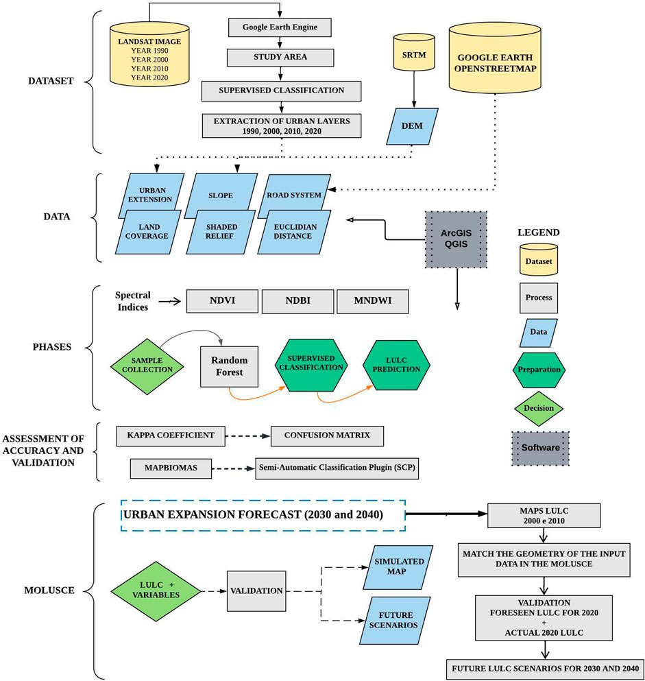
FIGURE 1. Methodology flowchart.
The Porto Alegre Metropolitan Region (RMPA) is located in the Rio Grande do Sul state in Brazil (Figure 2). The RMPA was created in 1973 by Federal Complementary Law 14/73, currently comprises 34 municipalities with 10,335 km2, and is Brazil’s fifth most populous metropolitan region. The RMPA is a pole of attraction and integration for political and socioeconomic dynamics. Previously, this characteristic was primarily observed in Porto Alegre and the most populous cities, but it has now extended to the surrounding municipalities. The RMPA experiences significant economic expansion as many individuals are drawn to the region by employment opportunities. This flux of people has contributed to the area’s robust economic growth within the state over the years (Secretaria de Planejamento, 2020).
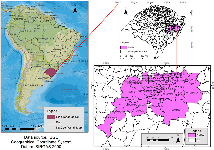
FIGURE 2. Porto Alegre Metropolitan Region (RMPA) location.
In this study, satellite data from Landsat-5 (sensor: TM) for the years 1990 and 2000, Landsat-7 (sensor: TM+) for the year 2010, and Landsat-8 (sensor: OLI) for the year 2020 were chosen between June and October to minimize visual obstruction caused by cloud cover. These datasets were accessed automatically from the United States Geological Survey (USGS) database within the GEE platform.
The independent spatial variables for the CA-ANN model for the future scenarios in this study were constructed using the road, railway network data, the Porto Alegre capital location, the other municipality’s downtown locations, and a Digital Elevation Model (DEM). These spatial variables were integrated into the model to capture and represent relevant geographical and transportation features of the study area.
This study’s declivity (slope) and shaded relief data were derived from the Shuttle Radar Topography Mission (SRTM) Digital Elevation Model at a 30 m spatial resolution. This data was downloaded from the NASA Earth Data website (https://search.earthdata.nasa.gov/) and accessed in June 2022. These data provide information about the slope and the terrain shade, essential variables for analyzing LULC changes in the study area. The vector layers of roads, railway stations, and municipal downtown locations were obtained from the OpenStreetMap project (https://www.openstreetmap.org/), an independent mapping collaborative project which provides freely accessible data.
This study calculated several Euclidian distance maps based on the vector layers, including the distance to the road, railway structures, the city’s downtown, and the capital Porto Alegre (Figure 3). Calculating these distances provides valuable spatial information and helps analyze the relationship between LULC changes and their proximity to transportation infrastructure and urban centers. According to Sajan et al. (2022), road and railway stations significantly shape the LULC dynamic conditions. These transportation infrastructure layers can influence LULC changes and patterns in a given area. The roads and railroads can impact accessibility, urban expansion, and the spatial distribution of different land use categories. Therefore, considering their influence is essential in understanding and predicting future LULC dynamics.

FIGURE 3. (A) altimetry; (B) slope; (C) shaded relief; (D) distance from Porto Alegre; (E) distance from railway stations; (F) distance from urban centers; (G) distance from roads.
Cloud masking was employed to remove both cloud coverage and their corresponding shadows from each time series collection. This technique eliminates all contaminated pixels caused by cloudiness or no-data conditions, ensuring that only clear and useable data is retained for further analysis (Langner et al., 2018; Pimple et al., 2018). By eliminating the cloud’s influence, the accuracy and reliability of subsequent analyses and interpretations are significantly improved.
Next, the data from multiple sources for each time slot were combined into specific data stacks using the median filter, a common technique used in image processing to reduce noise and preserve spatial data integrity. By applying it, the resulting data stacks represent the median values of the input data, effectively decreasing the outlier’s impact and enhancing the dataset’s overall quality.
For the supervised classification process, in addition to the conventional bands (B2, B3, B4, and B5 for all the Landsat family sensor collections), spectral indices such as the Normalized Difference Vegetation Index (NDVI), Normalized Difference Built-Up Index (NDBI), and Modified Normalized Difference Water Index (MNDWI) were used.
These spectral indices provide additional information that helps distinguish different LULC classes. The NDVI is commonly used to assess vegetation density and health, with higher values indicating denser and healthier vegetation Eq. 1. The NDBI highlights built-up areas, with higher values indicating a higher proportion of built-up surfaces Eq. 2. The MNDWI is sensitive to water bodies, with higher values indicating the water presence Eq. 3. Although NDWI is widely used to detect water bodies, MNDWI performs better when the water body is mixed with vegetation (Xu, 2006). Therefore, incorporating these indices into the classification process allows a more LULC comprehensive analysis, capturing essential characteristics related to vegetation, built-up areas, and water bodies, which can improve the accuracy and effectiveness of the classification results.
where red (RED), near-infrared (NIR), green (GREEN), and short-wave infrared (SWIR1) are the satellite’s bands. These three spectral indices were added as three bands to each image stack. Finally, the new stacked image was then used in the RF classifier.
The LULC classes used in this study were Cropland, Built-up, Grasslands, Water, Natural Forest, and Planted Forest. Approximately 300–400 polygonal samples were obtained for each class in the classification process. The samples were divided into two sets: 70% were randomly selected for model training, while the remaining 30% were used to validate the LULC maps. These polygons were uniformly selected across the study area, with the assistance of high-resolution Google Earth images.
According to Breiman (2001), the RF classification algorithm is based on an ensemble learning technique that combines multiple independent decision trees into a single model. Each tree in the RF is trained on a random dataset subset, where a data subsample is randomly selected for training. The tree is constructed during the process by recursively partitioning the dataset into smaller subsets based on decision rules derived from the data’s features. Each node corresponds to a question about the data, and each branch represents a possible answer. This building tree process enables the model to learn the relationship between the features of the data and their respective classes. During the classification phase, each tree is utilized to classify the image independently, and the final classification is determined by aggregating the results of all the trees and assigning the most common class to each pixel.
In the remote sensing image classification, two adjustable parameters are crucial in the algorithm: the decision trees number to be generated and the minimum number of nodes. These parameters are considered “floating” because their values can be adjusted based on the data-specific characteristics and the desired classification results. Although, studies such as Pelletier et al. (2016) indicate that the change in parameter values interferes little with the final model outcome. In this sense, the decision tree value was set as 50.
After generating the classification results, addressing local noise, commonly referred to as the “salt and pepper” effect, in the pixel-based classification is recommended. This can be achieved by applying a smoothing process using a moving window of size three on the classified image. The smoothing can be performed iteratively in three iterations using the majority vote rule. Therefore, this approach was conducted and helped reduce the impact of isolated misclassifications and improve the overall accuracy of the classification.
As Huang et al. (2017) described, a contingency or confusion matrix was created using 30% of the sample data reserved for validation to assess the accuracy of the LULC classifications. The confusion matrix compares the predicted classes with the actual classes and comprehensively assesses the classification performance. It consists of cells representing the counts of true positives and negatives, false positives and negatives. By analyzing the values in the matrix, various accuracy metrics can be calculated, such as overall, producer’s, and user’s accuracies and the Kappa index (K). This evaluation process helps in understanding the quality and reliability of the classification results and identifying areas of improvement if necessary.
A confusion matrix is an algorithm built into GEE, which validates and evaluates the image classification accuracy. With the confusion matrix, the K and overall accuracy (OA) are calculated Eqs 4–6:
where N refers to the rows and columns number in the error matrix, Xii corresponds to the number of observations in row i and column i, xi+ is the row i marginal total, and X + i equals the column i marginal total.
The User Accuracy (UA) for each class is assessed by the proportion of pixels correctly associated with a given class relative to the total number of classified pixels. Similarly, Producer Accuracy (PA) is determined by the ratio of correctly classified pixels to the total number of pixels in the reference data in each LULC class. Proportional error reduction is determined by comparing the errors of a classification class to the errors of a completely random class. Typically, the magnitude ranges from −1 to +1. The coherence level is considered adequate when it is greater than + 0.5. The statistics used to evaluate the accuracy of LULC maps are metrics established in the literature (Jensen and Cowen, 1999; Congalton and Green, 2009).
The Kappa index is widely used for evaluating the LULC classification’s accuracy. However, as mentioned in studies such as Foody (2010), it has certain limitations and considerations that should be considered when interpreting its results. It measures the agreement between the observed classifications and the reference data, considering the agreement that could occur by chance. It considers the confusion matrix’s diagonal (agreement) and off-diagonal (disagreement) elements. Usually, the K can be influenced by class frequency distribution, sample size, and confusion matrix structure. For example, if a particular class is highly dominant or rare in the dataset, it may disproportionately affect the results. Despite these limitations, the K is still widely used as an indirect indicator of classification accuracy, providing a single value that summarizes the agreement between the classified map and the reference data. However, interpreting it with other accuracy measures and considering the dataset-specific characteristics and classification process limitations is essential.
This study utilized the MOLUSCE plugin, which operates within the QGIS 2.18.10 software, to develop future LULC scenarios for the RMPA region in 2030 and 2040. The prospective model employed the ANN-CA method, which offers several advantages, including its ability to handle complex data, exhibit strong prediction performance, and require minimal pre-processing of input data (Abbas et al., 2021).
Pearson’s coefficient was estimated to evaluate the linear correlation between the independent geographic variables, LULC spatial-temporal changes conditioners. This coefficient ranges from −1 to +1, where −1 indicates a perfect negative correlation, +1 indicates a perfect positive correlation, and 0 indicates no linear correlation between the variables. After calculating Pearson’s coefficient, it was found that the variables with the highest correlation with each other include the distance from stations and roads, urban centers and Porto Alegre, shaded relief and distance from roads, distance from urban centers and shaded relief.
To correctly develop future scenarios, preparing the input layers must demand special attention from the users since the input layers’ inconsistencies in geometry, pixel size, and projection affect the results. Thus, all dependent and independent variables were set to contain the exact spatial resolution of 30 m/pixel and SIRGAS2000 Datum, 23 S UTM zone projection. Among the simulation models, the ANN seeks to establish a sigmoid function numpy. tanh, which is responsible for resizing the intervals of the transition categories to (y 1,1) during the configuration of the predictive scenarios (Rahman et al., 2017).
This model encompasses the complex dynamic relationships logic, which has proven to be highly suitable for modeling temporal transformations in land use as described in the works of Perović et al. (2018), and six steps support its execution model, the first being the loading of inputs comprising the LULC layers associated with the RMPA physical-social characterization layers.
In the next step, the level of correlation between the first period and the second period are quantified through the consistency values present in the intersection between the independent variables, which can be calculated through Pearson’s equation, Crammer’s coefficient, or uncertainty of the joint information. In the third step, the quantitative changes in the area of the use and cover classes between 2000 and 2010 are stipulated, as well as their expansion or retraction process, represented in km2.
In addition to generating a transition map that is responsible for guiding the next step, focused on modeling the transition potential, being the basis for applying the ANN, MLP, which operates the transition model based on the collection of input variables, guided by additional parameters provided by the user, aiming to optimize the ANN training model to obtain the most reliable result regarding the 2020 usage and coverage scenario, the trial and error process was adopted in the parameter adjustments during the fourth step, getting the following optimized parameters: Iteration rate: 1,000, Learning rate: 0.001, Momentum: 0.03, Neighborhood: 10 px, Hidden layer: 11. The prediction for the 2020 usage and coverage scenario was performed using the CA simulation stage (Hakim et al., 2019).
After generating the projection map for the year 2020, it was compared to the observed LULC map generated by the Randon Forest classifier in the GEE for the same year. This comparison aimed to evaluate the ANN-CA model prediction performance, then the validation assessment was employed to calculate the Histogram Kappa (HisK) Eq. 7, Overall Kappa (OvK) Eq. 8, Location Kappa (LocK) Eq. 9 metrics, and the percentage of correction Eqs 10, 11. These metrics play a crucial role in determining the model’s performance.
Where, HisK is the kappa histogram value for the specific class “i”, iPmax i is the maximum observed proportion of agreement for the specific class “i”, and iP(E) is the expected proportion of agreement for the specific class “ i”.
Where, OvK is the overall kappa coefficient, P(A) is the observed proportion of agreement, and P(E) is the expected proportion of agreement.
Where, LocK is the kappa location coefficient, P(A) is the observed proportion of agreement, P(E) is the expected proportion of agreement, and Pmax is the maximum observed proportion of agreement.
Where, Pii is the proportion of units correctly classified for the specific class “i”, PiT is the proportion of units of class “i” observed in the reference classification, PTi is the proportion of units of class “i” observed in the evaluated classification, P(A) is the correction percentage, “c” is the total number of classes, and PMax is the maximum possible value of P(A), considering all classes.
Afterward, the spatial similarity and consistency between them can be assessed by comparing the actual LULC map with the future scenarios generated by the CA-ANN model. The LoK quantifies their spatial similarity relationship, indicating how well they align in spatial distribution. On the other hand, the OvK assesses the simulation performance, considering both spatial and non-spatial comparison aspects. Both cases range between 0 and 1, where values closer to 1 indicate a higher agreement, whereas values closer to 0 show a lower agreement between the compared factors. The procedures were performed iteratively, using the trial and error method. Therefore, several calibrations were tested on the model parameters until the desired accuracy was achieved.
After obtaining the desired accuracy in the validation stage, the future LULC projection scenarios for 2030 and 2040 began the last modeling stage. Initially, the value of “n” in the time transition module was modified to 2 and 3 in the Input tab of the plugin. This adjustment was made to generate predictions when the input was set as 2000 for the initial year and 2010 as the final year. The ANN spatiotemporal model transition was conditioned to be equivalent to 10 years, ensuring a consistent 10-year interval between the predicted years.
In order to measure the annual LULC change rate for the scenarios, the magnitude of change between the years of interest was calculated as the difference between the end year and the start year, then divided by the product between the start year and the period covered Eq. 12 (Muhammad et al., 2022).
where, ACR corresponds to the LULC class annual dynamics rate. Iy and Fy comprise the LULC class area volume quantifications for the initial and final year, respectively, and t is the time interval.
Through the “explain” function executed by the GEE cloud platform, each variable relevance level used for the LULC classification scenarios was identified. This function assigns contribution values to the variables based on the classification results, where higher values indicate greater importance (Yang et al., 2008). The normalized indices obtained intermediate scores for all four classification models performed, while a more dynamic relevance behavior is found in the spectral bands.
The LULC classes used in this study were Cropland, Built-up, Grasslands, Water, Natural Forest, and Planted Forest. The Random Forest algorithm was used to classify the LULC features corresponding to 1990, 2000, 2010, and 2020 years based on Landsat data and spectral indices. Each class in square kilometers (km2) for the RMPA is shown in Table 1, which provides a comprehensive overview of the spatial distribution and LULC changes over time, spatially illustrated in Figure 4. The results of the multitemporal statistical analysis of the LULC spatial dynamics in the RMPA showed that from 1990 to 2020, there was a linear growth of urban area and cropland, as can be seen in Table 1 which shows the area estimates and change statistics of LULC classes for each year under study.
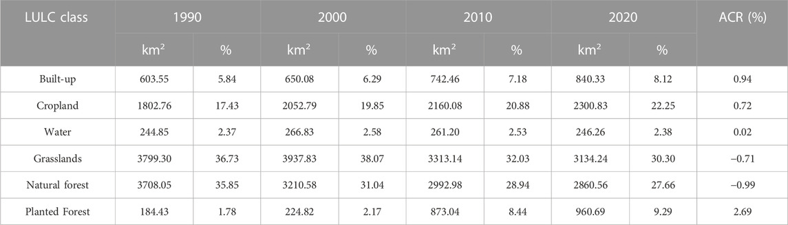
TABLE 1. LULC areas from 1990 to 2020 in km2 and annual change rate (ACR) in percentage.
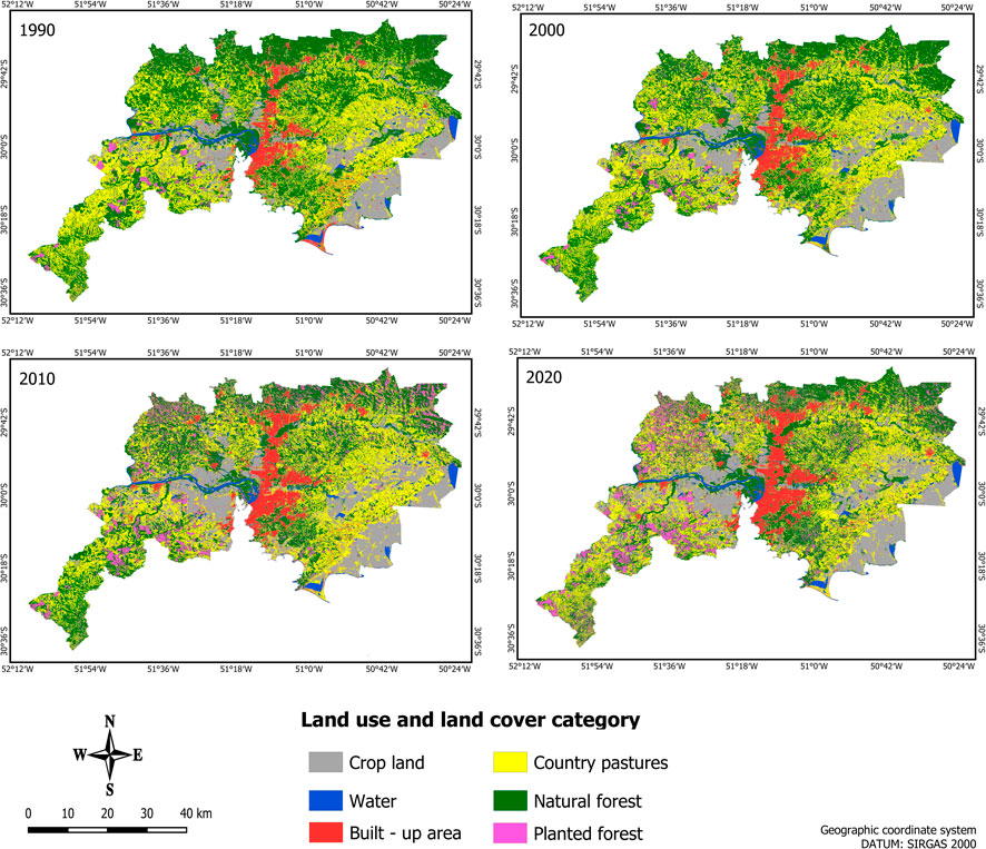
FIGURE 4. Relationship between the 1990–2020 LULC maps.
Kappa statistics, producer, consumer and global precision were used to evaluate the LULC maps derived from the supervised classification carried out in the GEE for the years 1990, 2000, 2010 and 2020, which reached an excellent average precision of 0.9. The highest overall accuracy and K were found in 1990, with 0.92 and 0.91, respectively. In 2000, 2010 and 2020, the overall accuracy and K values were 0.90 and 0.88, 0.90 and 0.88, 0.88 and 0.86, respectively. These results are in agreement with those found by Phan et al. (2020), who used the RF classifier to produce LULC maps with “moderate” to “high” accuracy, estimating overall accuracy levels between 0.84 and 0.89, using different satellite data, normalized indices, and radar data. The results observed by Talukdar et al. (2020) evaluate the classification potential of several machine learning and deep learning algorithms RF, SVM, ANN, Fuzzy Adaptive Resonance Theory-supervised predictive Mapping (Fuzzy ARTMAP), spectral angle mapper (SAM) and Mahalanobis Distance (MD), the results indicate that the RF algorithm estimated the highest accuracy levels, with 0.89.
Therefore, the accuracy values estimated in our classification for the RMPA can be considered excellent accordingly (Congalton and Green, 2009). For the commission and omission errors in 1990, the grassland class suffered the most pixel mixing with other classes, mainly cropland, reaching 24% and 15%, respectively. The same was observed for 2000 and 2010, with 28% and 17%, and 23% and 11%, consumer and producer errors, respectively. However, for 2020, the classes that showed the most pixel mixtures were natural and planted forests, with consumer and producer errors of 23% and 24%.
That way, the LULC classifications were consistent with the field reality. Some questions remained open, especially regarding the more suitable number of samples used in the validation process. In this study, the volume of samples presented in the confusion matrixes comprised 30% of the total volume of the samples collected, reaching from 300 to 400 polygons per class, which is usually used in other studies such as in Loukika et al. (2021), Pech-May et al. (2022). However, in other studies, much larger sample volumes have been used, such as in Yu et al. (2018). Therefore, we recommend that future studies test the accuracy values with different sample volumes to generate LULC validation.
LULC maps for the years 1990, 2000, 2010, and 2020, derived from Landsat TM/ETM+/OLI datasets and spectral NDVI, NDBI, and MNDWI indices, served as a basis for assessing the LULC class’s spatial dynamics in the RMPA. The variations and estimated percent area are presented in Table 2. Based on these data, it can be observed that the LULC feature corresponding to the built-up in the RMPA has undergone steady expansion since 1990, with a 0.9% annual increase rate.

TABLE 2. Temporal changes 1990–2020.
The most significant built-up area expansion was found between 2000 and 2010, approximately 14.2%, followed by the decade 2010–2020, 13.1%, and 1990–2000, 7.7%. In the last 30 years, from 1990 to 2020, the overall built-up area expansion was greater than 39.2%. The cropland area showed the most significant growth between 1990 and 2000, with a more than 13.8% increase. While in the two following decades, the area volume increased by 5.2% and 6.5% for the periods 2000 to 2010 and 2010 to 2020, respectively. In general, the cropland area showed an increase bigger than 27.6% from 1990 to 2020 and 0.7% annual rate.
In contrast, natural forests presented a linear decrease, which was most apparent between 1990 and 2000, reaching more than 13.4% suppression, followed by the decade 2010–2020, and 2000–2010, 4.4% and 6.7%, respectively. The native forest overall decrease in the RMPA from 1990 to 2020 was greater than 22.8% and about a 1.0% annual decrease rate. Although a natural forest area reduction has been observed over the decades, the suppression process is still linear, driven by built-up and cropland expansion. The grassland areas decreased significantly between 2000 and 2010, equivalent to approximately 15.8%, followed by the 2010–2020 decade, with a 5.4% decrease. However, it showed a considerable increase of more than 13.4% between 1990 and 2000. Even though the entire period of 1990–2020 presented a 17.5% grassland decrease and 0.7% annual decrease rate. Notably, the grassland areas in the RMPA have been replaced by built-up, cropland, and planted forest areas.
The water bodies are composed mainly of the Jacuí, Gravataí, Caí, and Sinos rivers, and in smaller expression lakes, ponds, and small dams. In this study, the water LULC class has not changed much over the years, which may be related to the precipitation volume in the reference years used to select the satellite images. During 1990 and 2000, the area increased by approximately 8.9%. However, from 2000 to 2010, there was a decrease greater than 2.1%; between 2010 and 2020, this decrease is even more significant, reaching more than 5.7%. In general, the water gain in the RMPA from 1990 to 2020 was only 0.58%, representing only a 0.02% annual rate increase.
In this study, the LULC class called “planted forest” indicated the spaces with Acacia, Eucalyptus, and Pinus forest crops, which are economically important for the Rio Grande do Sul state and Brazil’s national territory. The most significant increase occurred between 2000 and 2010, when the planted forest class more than doubled, followed by the 1990–2000 and 2010–2020 periods, with increases of 21.9% and 10.0%, respectively. The overall increase in planted forest from 1990 to 2020 more than quadrupled, and the annual growth rate was around 2.7%. The LULC spatial dynamic transition evaluation between 1990 and 2020 revealed a remarkable expansion in impervious surfaces and cropland to the detriment of forest and grassland (Table 2).
It can be seen that grassland, natural forests, cropland, planted forests, and water contributed 1.41%, 0.98%, 0.85%, 0.03%, and 0.02% to built-up class increase, respectively. The natural forest, along with the grassland, were the ones that contributed the most to the inter-class dynamics between 1990 and 2020. The natural forest lost about 0.98% of its areas to built-up, 2.34% to cropland, while the grassland areas received 4.34%, planted forest received 4.47%, and water body 0.16%. The grassland areas gave up about 1.41% of its areas to urban Infrastructure, 5.02% to cropland, 0.08% to water, 3.45% to natural forest, and 1.87% to planted forest.
If current trends continue, future LULC scenarios indicate that built-up will continue to happen in areas as close as possible to Porto Alegre and municipalities that offer more opportunities. This population and development concentration is driven by proximity to downtown, employment opportunities, and socioeconomic considerations. However, it is essential to conduct further analysis and consider other factors, such as infrastructure capacity, environmental sustainability, and urban planning strategies, to ensure these areas’ long-term viability and balanced growth since the results showed a decreasing trend in the natural landscape and an increase in built-up areas in the past and the future.
The transition matrix is critical for monitoring and understanding the LULC spatiotemporal dynamics. It can represent the number of pixels changed from one category to another. The matrix comprises rows and columns representing the LULC classes at the beginning and end of the studied period. The diagonal entries in the matrix are composed of each category stability level, i.e., the number of pixels that remained in the same category over the period studied. The off-diagonal entries represent the transitions from one category to another (Muhammad et al., 2022).
The transition matrix construction approach is especially suited for situations with a lot of ambiguity or challenges in implementing input data. From this process, an index is generated that ranks the landscape from zero to one, producing a consistent result, where values close to 1 in the diagonal entries represent the category stability, while values close to 0 indicate that significant changes during the period analyzed occurred (Sajan et al., 2022).
In the present study, the transition matrix’s applicability was essential for analyzing changes in the RMPA landscape over time, allowing the LULC changing pattern identification. The water and natural forest were the most stable in the first period, with change probabilities equivalent to 0.857 and 0.731, respectively. In contrast, grasslands, cropland, and planted forests had their stability levels reduced to 0.725, 0.660, and 0.468. It is worth mentioning that built-up presented a stability level of 0.689, and in the cropland and grassland, the main contributions were 0.047 and 0.027, respectively. In the second period, water and built-up had the highest stability levels, 0.835 and 0.824, respectively. The cropland, grassland, natural, and planted forests had reduced levels of transition stability, 0.647, 0.656, 0.656, and 0.631, respectively.
The classes that contributed the most to built-up remained cropland, 0.035, and grassland, 0.031. In the last period, the transition values for built-up and water were 0.846 and 0.810, respectively. In contrast, the values for cropland, grassland, natural, and planted forest were 0.687, 0.674, 0.665, and 0.419, respectively, similar to the first and second periods. Finally, the LULC classes that contributed the most to built-up were cropland, 0.038, and grassland, 0.029. During the study period, there was significant pressure on the natural forest and grassland areas, which had part of their areas absorbed by other LULC classes. The transition matrix between 1990 and 2000 shows this dynamic, with these being the classes with the lowest stability, 0.579 and 0.564, respectively.
Based on the LULC changes in historical data between 2000 and 2010, the CA-ANN method was used to project, in the first instance, the 2020 LULC condition with a 10-year phase extension and one iteration. Subsequently, the simulated 2020 LULC scenario was compared to the actual 2020 LULC obtained from the supervised classification using the RF algorithm (Figure 5) and Table 3. After the simulated model accuracy validation, the same CA-ANN framework was used and replicated to estimate the LULC scenarios for 2030 and 2040, presented in Figure 6 and Table 4.
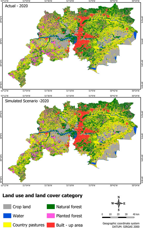
FIGURE 5. Current and projected LULC maps for 2020.

TABLE 3. Actual and projected LULC for 2020.
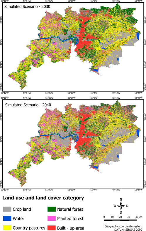
FIGURE 6. Predicted LULC maps for 2030 and 2040.
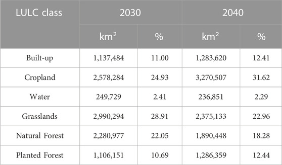
TABLE 4. Predicted area statistics in 2030 and 2040.
The estimated model accuracy measurement from the comparison between the LULC simulation projected for 2020 and the actual LULC for 2020 presented the HisK, OvK, and LoK of 0.80, 0.65, and 0.80, respectively, and 73.5% of percentage correctness. These results validate the simulation model’s suitability for predicting LULC future scenarios for the RMPA. For example, Muhammad et al. (2022) also used the CA-ANN approach in the MOLUSCE to analyze future spatiotemporal changes for Linyi, China, in 2030, 2040, and 2050 and got a LocK of 0.97, an percent of correctness of 65.80%, and an OvK value of 0.48. Another study for future LULC scenarios of 2030, 2040, and 2050 in Guangdong Hong Kong Macau, China got a validation OvK of 0.76, an percent of correctness of 96.25%, and LocK of 0.94 (Abbas et al., 2021). While in Dehingia et al. (2022), the validation indices were: HisK of 0.89, OvK of 0.61, and LocK of 0.69, with a 72.81% percent of correctness to estimate the future condition of 2029 for the Balikpapan City, Indonesia. In Gao et al. (2023), the future LULC scenarios in the Greater Yellow River region obtained an OvK of 0.94, HisK of 0.98, LocK of 0.95, and 96.42% percent of correctness. Therefore, we can infer that our simulation validation results are suitable for estimating the future LULC conditions for 2030 and 2040 in the RMPA.
The future scenario for 2030 and 2040 shows the cropland, built-up, and planted forests as the main LULC expanding classes (Table 5). The results indicate that by 2030, the cropland areas will show an increase of more than 12.0% compared to the 2020 actual scenario, equivalent to a 1.2% annual rate increase. For 2040, cropland areas are projected to still increase, reaching more than 42.1% of the 2020 area, indicating a 2.1% yearly growth rate and a 122.6% increase compared to the 2030 scenario. In addition, for the 2030 to 2040 period, an annual 2.6% growth rate is projected. Similarly, the model predicts a linear expansion for planted forest areas, with a 15.1% expansion for 2030, a 1.5% annual rate, and a 33.9% increase for 2040, reaching about 1.7% yearly growth concerning 2020. It is worth mentioning that planted forests will increase by about 16.3% in 2040 compared to 2030, reflecting a 1.6% annual growth rate between the years.
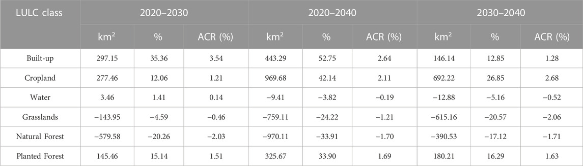
TABLE 5. LULC temporal changes in 2020 and 2040.
In turn, built-up areas will also increase in future scenarios, reaching more than 35.3% in 2030, compared to 2020, reaching a 3.5% annual growth rate, the highest recorded for this time series. Whereas in 2040, it will present a 52.7% increase indicating a yearly expansion rate of 2.6%. It is worth noting that despite maintaining a built-up growth trend in 2040, with a positive annual rate of 1.28%, this increase was 12.8%, reaching a 63.6% smaller area advance than that observed from 2020 to 2030.
Regarding the other LULC class’s prediction for 2030 and 2040, the most significant decrease occurred for the natural forest, which in 2030 will present an area loss corresponding to 20.2% concerning 2020, reaching a 2.0% annual rate decrease. While in 2040 a loss of natural forest equivalent to 33.9% is estimated compared to the 2020 scenario, getting a 1.70% yearly rate loss for the same period. Following the same trend, the grassland will present a decrease of about 4.6% in its by the year 2030, concerning 2020, keeping a 0.4% annual rate, and for 2040, a 24.2% reduction related to 2020, indicating a 1.2% yearly loss.
For the water, an 1.41% area increase is forecast for 2030 concerning 2020, indicating a 0.14% annual gain. In contrast, for 2040, a loss of 3.8% is estimated, reaching a 0.19% yearly decrease. According to the future scenarios, the LULC changes will adversely impact environmental and socioeconomic structures, mainly with cropland and built-up areas, in contrast with decreased vegetation and water. Similar trends are found in other studies worldwide, such as in Muhammad et al. (2022), Padma et al. (2022), Barwicka and Milecka (2022), Sajan et al. (2022), and Gao et al. (2023). Therefore, indications that the LULC changes behavior obtained for the RMPA follow a similar trend to those observed in other regions around the globe.
Regarding the contribution of LULC in built-up areas for future scenarios from 2030 to 2040 in the RMPA, there was a variation of cultivated area, pasture and natural forest of 1.7%, 0.6% and 1.3% for built-up areas, respectively. In addition, grassland was the class that contributed the most change, reaching 6.1% for cropland, while the natural forest class contributed 2.4% for planted forests increase. Therefore, this study can help formulate a better land use management policy in the Metropolitan Region of Porto Alegre. Furthermore, the study demonstrates the ability of the CA-ANN model to develop future LULC scenarios and understand the spatiotemporal changes. So, combining satellite remote sensing data with GIS has generated much interest due to concerns about the LULC dynamics (Lambin et al., 2001).
This research aimed first to determine the spatiotemporal dynamics present in LULC classes between 1990 and 2020 and second to develop future LULC scenarios for 2030 and 2040 for the Metropolitan Region of Porto Alegre (RMPA), located in the Rio Grande do Sul state, Brazil. Therefore, the Random Forest algorithm in the GEE cloud processing environment was used for the first aim to classify LULC conditions for 1990, 2000, 2010, and 2020 from Landsat, TM, ETM+, and OLI data, respectively, reaching an excellent global accuracy of 0.92, 0.90, 0.90, 0.88 for the years under study. Then, the LULC simulation was successfully estimated and validated for 2020, and the CA-ANN model was used to develop the 2030 and 2040 future LULC scenarios in the RMPA in the second aim, reaching a 0.65 overall Kappa index, 0.80 histogram Kappa, 0.80 Location Kappa and 73.50% percentage of correctness.
Thesethe findings in the validation statistics make it possible to infer that the model demonstrates good effectiveness in prospecting the LULC spatial conditions. The future scenarios regarding LULC changes for 2030 and 2040 highlighted that built-up, cropland and planted forests will be together the most representative areas along the RMPA boundaries, reaching 46.6% and 56.4%in 2030 and 2040, respectively. The built-up stands out as having the highest expansion rate in the area, reaching 35.3% and 52.3% increase in 2030 and 2040, respectively. In contrast, in the same period in 2030, natural forests will lose the largest area, suffering an area decline of 20.26%, followed by the grassland that will lose about 4.6% of its area in 2020.
In addition, by 2040, the natural forest loss is expected to be approximately 33.9%, followed by the grassland loss of 24.2% concerning 2020. Therefore, the present study highlights the relevance of monitoring the past and developing future LULC scenarios. Moreover, similar LULC pattern behaviors observed in the RMPA were also found in other regions of the country and the world, indicating that the methodology in this study could be replicated in other metropolitan regions.
The results obtained through modeling and predicting landscape patterns highlighted the need to consider physical elements and factors such as development policies and climatic conditions for a more comprehensive understanding of the LULC transitional dynamics in future studies. Therefore, it is suggested that future research incorporate a wide range of factors and data to deepen the knowledge of the effects of these elements on landscape patterns. Such more comprehensive investigations will be crucial to informing land managers and risk decision-makers, enabling the development of effective plans to mitigate the climate change impact and promote more sustainable use of the environment.
Understanding the built-up sprawl effect is essential to plan and develop better cities. This study took into account significant factors influencing urban sprawl. The variables used in the CA-ANN model were critical determinants as they significantly affected the LULC change mechanism. Based on the results, it is understood that the factors used were shown to be very influential in the way in which urban sprawl occurred and may continue to occur.
The raw data supporting the conclusion of this article will be made available by the authors, without undue reservation.
AF and FA conducted the study, prepared the data, performed the analysis, wrote the article, discussed the results and contributed to the final manuscript. VN supervised the project, verified the analytical methods, discussed the results and contributed to the final manuscript. JO checked the methods, discussed the results and contributed to the final manuscript. All authors contributed to the article and approved the submitted version.
This research was funded by Fundação de Amparo à Pesquisa do Estado de São Paulo (FAPESP) project number (2017/22269-2) and by Global Programme of Action for the Protection of the Marine Environment from Landbased Activities of the United Nations Environment Program (GPA/UNEP, no 2500116256) in support of the project Towards the Establishment of an International Nitrogen Management System (INMS).
The authors would like to thank the Coordenação de Aperfeiçoamento de Pessoal de Nível Superior (CAPES) process number (88882.438974/2019-01), the Fundação de Amparo à Pesquisa do Estado de São Paulo (FAPESP) project number (2017/22269-2). The the Global Program of Action for the Protection of the Marine Environment against Land Activities of the United Nations Environment Program (GPA/UNEP, no. 2500116256) in support of the project Towards the Establishment of an International Nitrogen Management System (INMS). The Graduate Program in Remote Sensing at Federal University of Rio Grande do Sul, the Federal University University of ABC in Brazil.
The authors declare that the research was conducted in the absence of any commercial or financial relationships that could be construed as a potential conflict of interest.
All claims expressed in this article are solely those of the authors and do not necessarily represent those of their affiliated organizations, or those of the publisher, the editors and the reviewers. Any product that may be evaluated in this article, or claim that may be made by its manufacturer, is not guaranteed or endorsed by the publisher.
Abbas, Z., Yang, G., Zhong, Y., and Zhao, Y. (2021). Spatiotemporal change analysis and future scenario of LULC using the CA-ANN approach: A case study of the greater bay area, China. Land 10, 584. doi:10.3390/land10060584
Alam, N., Saha, S., Gupta, S., and Chakraborty, S. (2021). Prediction modelling of riverine landscape dynamics in the context of sustainable management of floodplain: A geospatial approach. Ann. GIS 27 (3), 299–314. doi:10.1080/19475683.2020.1870558
Arsanjani, J. J., Kainz, W., and Mousivand, A. J. (2011). Tracking dynamic land-use change using spatially explicit Markov chain based on cellular automata: the case of Tehran. Int. J. Image Data Fusion 2 (4), 329–345. doi:10.1080/19479832.2011.605397
Ashaolu, E. D., Olorunfemi, J. F., and Ifabiyi, I. P. (2019). Assessing the spatio-temporal pattern of land use and land cover changes in osun drainage basin, Nigeria. J. Environ. Geogr. 12 (1–2), 41–50. doi:10.2478/jengeo-2019-0005
Barwicka, S., and Milecka, M. (2022). The "perfect village" model as a result of research on transformation of plant cover—case study of the puchaczów commune. Sustainability 14, 14479. doi:10.3390/su142114479
Batty, M. (1997). Cellular automata and urban form: A primer. J. Am. Plan. Assoc. 63 (2), 266–274. doi:10.1080/01944369708975918
Bhatta, B. (2010). Analysis of urban growth and sprawl from remote sensing data. Berlin/Heidelberg, Germany: Springer.
Chen, Y., Li, X., Liu, X., Ai, B., and Li, S. (2016). Capturing the varying effects of driving forces over time for the simulation of urban growth by using survival analysis and cellular automata. Landsc. Urban Plan. 152, 59–71. doi:10.1016/j.landurbplan.2016.03.011
Clarke, K. C., Hoppen, S., and Gaydos, L. (1997). A self-modifying cellular automaton model of historical urbanization in the San Francisco Bay area. Environ. Plan. B Plan. Des. 24 (2), 247–261. doi:10.1068/b240247
Congalton, R. G., and Green, K. (2009). Assessing the accuracy of remotely sensed data: Principles and practices. Boca Raton: CRC Press.
Dehingia, H., Das, R. R., Abdul Rahaman, S., Surendra, P., and Hanjagi, A. D. (2022). “Decadal transformation of land use land cover and future spatial expansion in Bangalore metropolitan region, India: open-source geospatial machine learning approach,” in The International Archives of the Photogrammetry, Remote Sensing and Spatial Information Sciences. XLIII-B3-2022, Nice, France, 6–11 June 2022. doi:10.5194/isprs-archives-XLIII-B3-2022-589-2022
Foody, G. M. (2010). Assessing the accuracy of land cover change with imperfect ground reference data. Remote Sens. Environ. 114 (10), 2271–2285. doi:10.1016/j.rse.2010.05.003
Gao, C., Cheng, D., Iqbal, J., and Yao, S. (2023). Spatiotemporal change analysis and prediction of the great Yellow River region (GYRR) land cover and the relationship analysis with mountain hazards. Land 12, 340. doi:10.3390/land12020340
Guidigan, M. L. G., Sanou, C. L., Ragatoa, D. S., Fafa, C. O., and Mishra, V. N. (2019). Assessing land use/land cover dynamic and its impact in Benin republic using land change model and CCI-lc products. Earth Syst. Environ. 3 (1), 127–137. doi:10.1007/s41748-018-0083-5
Hakim, A. M. Y., Baja, S., Rampisela, D. A., and Arif, S. (2019). Spatial dynamic prediction of landuse/landcover change (case study: tamalanrea sub-district, makassar city). IOP Conf. Ser. Earth Environ. Sci. 280, 012023. doi:10.1088/1755-1315/280/1/012023
Hu, Z., and Lo, C. P. (2007). Modeling urban growth in Atlanta using logistic regression. Comput. Environ. Urban Syst. 31 (6), 667–688. doi:10.1016/j.compenvurbsys.2006.11.001
Huang, D., Xu, S., Sun, J., Liang, S., and Wang, Z. (2017). Accuracy assessment model for classification result of remote sensing image based on spatial sampling. J. Appl. Remote Sens. 11, 1–13. doi:10.1117/1.jrs.11.046023
IBGE (2020). Agência IBGE notícias. Available at: https://agenciadenoticias.ibge.gov.br/agencia-noticias/2012-agencia-de-noticias/noticias/31471-ibge-lanca-colecao-de-mapas-municipais-2020.
Jensen, J. R., and Cowen, D. C. (1999). Remote sensing of urban/suburban Infrastructure and socioeconomic attributes. Remote Sens. Environ. 68 (1), 1–3.
Lambin, E. F., Turner, B., Geist, H. J., Agbola, S. B., Angelsen, A., Bruce, J. W., et al. (2001). The causes of land-use and land-cover change: moving beyond the myths. Glob. Environ. Chang. 11, 261–269. doi:10.1016/s0959-3780(01)00007-3
Langner, A., Miettinen, J., Kukkonen, M., Vancutsem, C., Simonetti, D., Vieilledent, G., et al. (2018). Towards operational monitoring of forest canopy disturbance in evergreen rain forests: A test case in continental southeast asia. Remote Sens. 10 (4), 544. doi:10.3390/rs10040544
Li, X., Lin, J., Chen, Y., Liu, X., and Ai, B. (2013). Calibrating cellular automata based on landscape metrics by using genetic algorithms. Int. J. Geogr. Inf. Sci. 27 (3), 594–613. doi:10.1080/13658816.2012.698391
Li, X., and Yeh, A. G. O. (2002). Neural-network-based cellular automata for simulating multiple land use changes using GIS. Int. J. Geogr. Inf. Sci. 16 (4), 323–343. doi:10.1080/13658810210137004
Ligtenberg, A., Bregt, A. K., and Van Lammeren, R. (2001). Multi-actor-based land use modelling: spatial planning using agents. Landsc. Urban Plan. 56 (1–2), 21–33. doi:10.1016/S0169-2046(01)00162-1
Loukika, K. N., Keesara, V. R., and Sridhar, V. (2021). Analysis of land use and land cover using machine learning algorithms on Google Earth engine for munneru river basin, India. Sustainability 13, 13758. doi:10.3390/su132413758
Meraj, G., Kanga, S., Ambadkar, A., Kumar, P., Singh, S. K., Farooq, M., et al. (2022). Assessing the yield of wheat using satellite remote sensing-BasedMachine learning algorithms and SimulationModeling. Remote Sens. 14, 3005. doi:10.3390/rs14133005
Mishra, V. N., and Rai, P. K. (2016). A remote sensing aided multi-layer perceptron-Markov chain analysis for land use and land cover change prediction in Patna district (Bihar), India. Arab. J. Geosci. 9, 1–18. doi:10.1002/9780470979587.ch22
Muhammad, R., Zhang, W., Abbas, Z., Guo, F., and Gwiazdzinski, L. (2022). Spatiotemporal change analysis and prediction of future land use and land cover changes using QGIS MOLUSCE plugin and remote sensing big data: A case study of Linyi, China. Land 11, 419. doi:10.3390/land11030419
Padma, S., Vidhya Lakshmi, S., Prakash, R., Srividhya, S., Sivakumar, A. A., Divyah, N., et al. (2022). Simulation of land use/land cover dynamics using Google Earth data and QGIS: A case study on outer ring road, southern India. Sustainability 14, 16373. doi:10.3390/su142416373
Pech-May, F., Santos, R. A., Toledo, G. R., and Duran, J. P. F. P. (2022). Mapping of land cover with optical images, supervised algorithms, and Google Earth engine. Sensors 22, 4729. doi:10.3390/s22134729
Pelletier, C., Valero, S., Inglada, J., Champion, N., and Dedieu, G. (2016). Assessing the robustness of Random Forests to map land cover with high resolution satellite image time series over large areas. Remote Sens. Environ. 187, 156–168. doi:10.1016/j.rse.2016.10.010
Perović, V., Jakšić, D., Jaramaz, D., Koković, N., Čakmak, D., Mitrović, M., et al. (2018). Spatio-temporal analysis of land use/land cover change and its effects on soil erosion (Case study in the Oplenac wine-producing area, Serbia). Environ. Monit. Assess. 190 (11), 675. doi:10.1007/s10661-018-7025-4
Phan, T. N., Kuch, V., and Lehnert, L. W. (2020). Land cover classification using Google Earth engine and random forest classifier-the role of image composition. Remote Sens. 12 (15), 2411. doi:10.3390/rs12152411
Pimple, U., Simonetti, D., Sitthi, A., Pungkul, S., Leadprathom, K., Skupek, H., et al. (2018). Google Earth engine based three decadal Landsat imagery analysis for mapping of mangrove forests and its surroundings in the trat province of Thailand. J. Comput. Commun. 6, 247–264. doi:10.4236/jcc.2018.61025
Prenzel, B. (2004). Remote sensing-based quantification of land-cover and land-use change for planning. Prog. Plan. 61, 281–299. doi:10.1016/s0305-9006(03)00065-5
Rahman, M., Tabassum, F., Rasheduzzaman, M., Saba, H., Sarkar, L., Ferdous, J., et al. (2017). Temporal dynamics of land use/land cover change and its prediction using CA-ANN model for southwestern coastal Bangladesh. Environ. Monit. Assess. 189, 565. doi:10.1007/s10661-017-6272-0
Sajan, B., Mishra, V. N., Kanga, S., Meraj, G., Singh, S. K., and Kumar, P. (2022). Cellular automata-based artificial neural network model for assessing past, present, and future land use/land cover dynamics. Agronomy 12, 2772. doi:10.3390/agronomy12112772
Saputra, M. H., and Lee, H. S. (2019). Prediction of land use and land cover changes for North Sumatra, Indonesia, using an artificial-neural-network-based cellular automaton. Sustain. Switz. 11 (11), 1–16. doi:10.3390/su11113024
Secretaria De Planejamento (2020). Atlas socioeconômico do Rio Grande do Sul. Available at:https://atlassocioeconomico.rs.gov.br/regiao-metropolitana-de-porto-alegre-rmpa.
Shi, W., and Pang, M. Y. C. (2000). Development of Voronoi-based cellular automata—an integrated dynamic model for Geographical Information Systems. Int. J. Geogr. Inf. Syst. 14 (5), 455–474. doi:10.1080/13658810050057597
Talukdar, S., Singha, P., Shahfahad, , Mahato, S., Praveen, B., and Rahman, A. (2020). Dynamics of ecosystem services (ESs) in response to land use land cover (LU/LC) changes in the lower Gangetic plain of India. Ecol. Indic. 112, 106121. doi:10.1016/j.ecolind.2020.106121
Vaz, E., de Noronha, T., and Nijkamp, P. (2014). Exploratory landscape metrics for agricultural sustainability. Agroecol. Sustain. Food Syst. 38 (1), 92–108. doi:10.1080/21683565.2013.825829
Wu, F., and Webster, C. J. (2000). Simulating artificial cities in a GIS environment: urban growth under alternative regulation regimes. Int. J. Geogr. Inf. Sci. 14 (7), 625–648. doi:10.1080/136588100424945
Xu, H. (2006). Modification of normalised difference water index (NDWI) to enhance open water features in remotely sensed imagery. Int. J. Remote Sens. 27 (14), 3025–3033. doi:10.1080/01431160600589179
Yang, Q., Li, X., and Shi, X. (2008). Cellular automata for simulating land use changes based on support vector machines. Comput. Geosciences 34 (6), 592–602. doi:10.1016/j.cageo.2007.08.003
Yu, Z., Di, L., Tang, J., Zhang, C., Lin, L., Genong, E., et al. (2018). “Land use and land cover classification for Bangladesh 2005 on Google Earth engine,” in 7th International Conference on Agro-geoinformatics (Agro-geoinformatics), Hangzhou, China, August 6-9, 2018, 1–5. doi:10.1109/Agro-Geoinformatics.2018.8475976
Keywords: predicted LULC, ANN-CA, GEE, MOLUSCE, scenarios
Citation: Fontana AG, Nascimento VF, Ometto JP and do Amaral FHF (2023) Analysis of past and future urban growth on a regional scale using remote sensing and machine learning. Front. Remote Sens. 4:1123254. doi: 10.3389/frsen.2023.1123254
Received: 13 December 2022; Accepted: 17 August 2023;
Published: 01 September 2023.
Edited by:
Erin Bunting, Michigan State University, United StatesReviewed by:
Rodrigo Rafael Souza De Oliveira, Universidade do Estado do Pará, BrazilCopyright © 2023 Fontana, Nascimento, Ometto and do Amaral. This is an open-access article distributed under the terms of the Creative Commons Attribution License (CC BY). The use, distribution or reproduction in other forums is permitted, provided the original author(s) and the copyright owner(s) are credited and that the original publication in this journal is cited, in accordance with accepted academic practice. No use, distribution or reproduction is permitted which does not comply with these terms.
*Correspondence: Andressa Garcia Fontana, YW5kcmVzc2FnZm9udGFuYTk0QGdtYWlsLmNvbQ==
Disclaimer: All claims expressed in this article are solely those of the authors and do not necessarily represent those of their affiliated organizations, or those of the publisher, the editors and the reviewers. Any product that may be evaluated in this article or claim that may be made by its manufacturer is not guaranteed or endorsed by the publisher.
Research integrity at Frontiers
Learn more about the work of our research integrity team to safeguard the quality of each article we publish.