Machine learning-enabled real-time detection of cloud and aerosol layers using airborne lidar

Lidar profiling of the atmosphere provides information on existence of cloud and aerosol layers and the height and structure of those layers. Knowledge of feature boundaries is a key input to assimilation models. Moreover, identifying feature boundaries with minimal latency is essential to impact operational assimilation and real-time decision making. Using advanced convolution neural network algorithms, we demonstrate real-time determination of atmospheric feature boundaries using an airborne backscatter lidar. Results are shown to agree well with traditional processing methods and are produced with higher horizontal resolution than the traditional method. Demonstrated using airborne lidar, the algorithms and process are extendable to real-time generation of data products from a future spaceborne sensor.

1 Introduction

One of the biggest strengths of lidar remote sensing is the inherent ability to provide vertically resolved profiles of cloud and aerosol features. Concomitantly, the ability to identify the height of an atmospheric feature (i.e., top/bottom of cloud or aerosol layer) is one of the most basic and easily achieved results obtained from lidar. Accurate height information is a critical and highly desired input parameter for atmospheric models [Marchand and Ackerman, 2010; Kipling and Co-authors, 2016; O’Sullivan et al., 2020; Krishnamurthy et al., 2021]. Using lidar, features can typically be resolved with vertical resolution (10s m) that easily exceeds the needs of models. Determining existence of a feature and feature height does not, to first order, require calibration or detailed retrieval methods although historically data is calibrated and then a thresholding method is applied to determine feature boundaries (as in, e.g., Yorks et al., 2011 or Hlavka et al., 2012). Higher-order data products, such as calibrated backscatter, optical depth, or extinction, are derived from lidar data by use of retrieval techniques (e.g., Klett, 1981) and ascribing a feature type (e.g., classifying type of cloud or aerosol) to a feature does, typically, require use of retrieval methods.

In the simplest form, determining feature heights is traditionally accomplished by defining a threshold to separate signal from noise. Thresholding is, however, subject to a degree of arbitrariness because the threshold has to be defined and, of course, as signal and noise levels change the threshold can change. Setting the threshold too high will result in loss of weaker signals and setting the threshold too low will allow noise to be claimed as features. Nevertheless, to-date the thresholding technique has persisted simply because it is easy to understand and implement, even if it does involve a degree of subjectiveness.

Assimilation of lidar vertical profiles can improve simulations of aerosol transport, but improved accuracy and, more critically, improved latency of lidar data products are required to implement the assimilation operationally and inform decisions during hazardous events. There are several operational or quasi-operational aerosol transport and air quality models that are critical tools for forecasting aerosol plume transport during hazardous events (Benedetti and Co-authors 2018). Proper estimation of aerosol vertical distributions remains a well-documented weakness in these models, yet is a key component of simulating transport (Janiskova et al., 2010; Zhang et al., 2011). Hughes et al (2016) shows that experimentally assimilating height estimates from space-based lidar into an aerosol transport model enabled more accurate 4-D volcanic ash dispersion forecasts. Without the accurate volcanic plume injection height provided by lidar, the placement of the mass is assumed using trajectory analysis, resulting in large uncertainties in the predictions. Operational global aerosol models are not currently assimilating lidar vertical profiles because there are no current space-based lidar sensors providing near-real-time (NRT) data products necessary to support this application. Additionally, lidar real-time data products are desired for Department of Defense (DoD) applications and for real-time decision-making by groups such as the Volcanic Ash Advisory Centers (VAACs) and US Forest Service. The science-enabling real-time data product capability presented in this paper meets the needs of these user communities.

2 Real-time feature detection

Finding atmospheric features in lidar data normally begins by subtracting undesired solar background noise. In traditional analysis, background signal from a range below the level of the Earth surface (i.e., thus guaranteed to be free of any laser-induced signal) is averaged and subtracted from each measured profile. While simple in concept and easy to implement, the resultant data can still be noisy owing to low signal levels. Previous work by Yorks et al (2021) described removal of residual background noise, or “denoising,” using artificial intelligence/machine learning (AI/ML) techniques as applied to spaceborne photon-counting lidar data. That paper demonstrated a substantial improvement in both number of layers detected and in horizontal resolution of the data product when the AI/ML analysis was used, although it was demonstrated using existing data sets. Work by Palm et al (2021) applied AI/ML algorithms to existing spaceborne data, detecting layer height and boundaries at greatly improved resolution. In this work we apply AI/ML-based algorithms for real-time detection of atmospheric features and determination of feature height during instrument operation. Initial application and testing was conducted using a high-altitude airborne lidar, but the extension to spaceborne lidar should be immediately apparent.

Convolution Neural Network (CNN) algorithms to produce real-time feature detection and layer height were developed and tested using the long-standing airborne Cloud Physics Lidar (CPL; McGill et al., 2002) instrument. Flying on the NASA ER-2 high-altitude aircraft, the CPL operates at 5 kHz repetition rate with data integrated to 10 Hz (corresponding to −20 m along-track horizontal resolution at typical aircraft speed of −200 m/s). Thus, the native resolution of CPL data is −20 m horizontal by 30 m vertical. The CPL instrument transmits a serial data stream of one subsampled data channel (normally 532 nm raw photon counts) that can be downlinked from the aircraft to a ground computer during science flights. Because the aircraft downlink only samples the data once per second, a single 10 Hz profile is transmitted once every second.

For these tests, the CPL serial data stream (10 Hz data rate subsampled at 1 Hz) was routed to a Nvidia Jetson TX2 board. In simple terms, a Jetson TX2 is a processor with an operating system (OS), so it functions like a normal computer. Designed for embedded systems, the TX2 board has input connectors to enable easy interface to the CPL serial real-time data feed. It has RAM memory on which code can be loaded that can be accessed and run by the processor. A data profile is received, via serial input line, from the CPL instrument. The Jetson also receives airplane navigation data (for altitude/pitch/roll/yaw) that is used to adjust the profile by calculating any altitude or pointing offset, which is especially necessary when the airplane banks into turns. The Jetson then applies the CNN to the accumulated CPL profiles (512 profiles) and outputs a corresponding binary image where detected layers are ‘one’ and non-layers are “zero”. The CNN algorithm was loaded on the Jetson board, and the resultant real-time data products were then transmitted to the ground, once per second, during operation. Figure 1 illustrates the overall flow of data collection and processing and the steps involved.

FIGURE 1

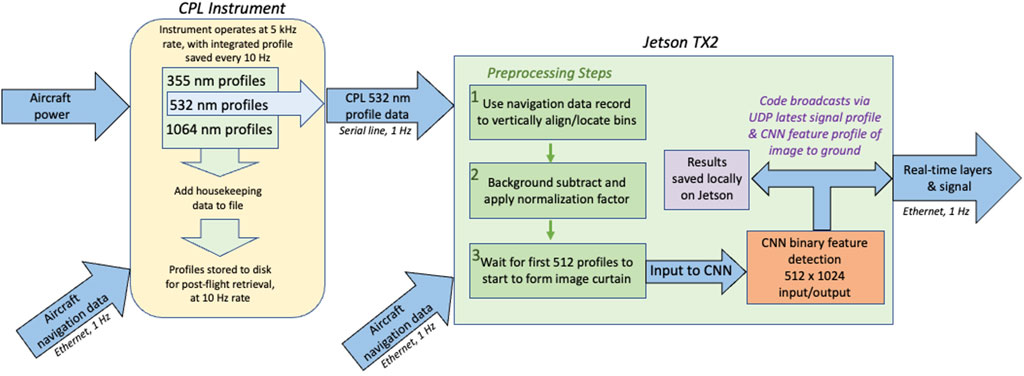
FIGURE 1. Overview of CPL data collection, data interfaces, and Jetson TX2 processing flow. Owing to bandwidth limitations on the aircraft data network, only one (of ten) CPL profiles per second is transmitted to the TX2 board.

A standard U-Net (Ronneberger et al., 2015) CNN was trained for binary feature detection on the CPL real-time data stream. Being two dimensional data (profiles of height by time), lidar data is well suited to processing by a CNN. Although CPL data are collected at 10 Hz, the real-time serial output is subsampled at 1 Hz owing to aircraft network limitations. Therefore, training data were sampled to 1 Hz to mimic the aircraft real-time data stream. The standard CPL layer detection product, produced at 5 s (∼1 km) resolution, was up-sampled back to 1 s to label the input signal (photon counts). Each input and output sample pair were 512 records (or profiles) horizontal by 1024 bins vertical. Extra bins are zero-padded since 1024 was the minimum power of two that accommodated the full vertical extent. Additional details of the CNN are shown in Table 1. Prior CPL data was used as training data (all CPL data is freely available at https://cpl.gsfc.nasa.gov). There was one training data set used, and its details are given in Table 1. However, because some prior flights were highly biased towards specific science targets (i.e., convective clouds or other specific targets), the training data were curated to avoid excessive frequencies of certain features and thereby create a better statistical balance of features that may be observed on any given flight. Although CPL data is high quality, standard definitions of ‘quality’ do not apply as the CNN only operates on normalized uncalibrated data.

TABLE 1

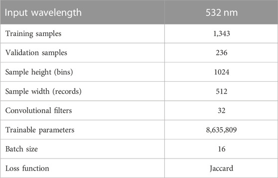
TABLE 1. Parameters used for the CNN.

The CPL raw photon count data (i.e., a profile of photon counts) enters the Jetson TX2 board via a serial input line. Navigation data from the aircraft is also fed into the Jetson TX2 board, and this allows real-time correction for aircraft pointing in pitch-roll-yaw. More importantly, it allows for vertical alignment of the profiles based on the aircraft GPS altitude. The next step is to subtract solar background signal from the profile. Given the relatively high signal-to-noise (SNR) in the airborne data, background is simply subtracted using an average value for the profile (not using the advanced denoising method). Then data are scaled (so it is in the same form as the training data) and input into the CNN feature detection algorithm. To accommodate the expected sample size of 512 records, upon first receiving data the algorithm must wait to accumulate 512 1-Hz profiles (8.53 min) of data. Afterward, the CNN performs feature detection every time it receives a new profile, which is notionally every second assuming no data dropouts. This detection interval is adjustable but was selected to allow ample margin for computation and downlink.

3 Initial results

The CPL instrument with the real-time data product capability was flown in the Investigation of Microphysics and Precipitation for Atlantic Coast-Threatening Snowstorms (IMPACTS) field campaign during January-February 2022 (McMurdie et al., 2022). Most flights were over thick convective cloud systems although many scenes displayed complex multi-layered structure. Figure 2 shows an example of such a scene from 8 February 2022. The top panel in Figure 2 shows the CPL 532 nm profiles of attenuated backscatter coefficient. The 532 nm profiles are the data fed to the Jetson TX2 board for real-time layer detection and height determination. The second panel in Figure 2 shows the layer finding results from standard CPL data processing (i.e., using traditional processing methods and at 5 s/1 km horizontal resolution). The bottom panel in Figure 2 displays the real-time AI/ML-derived layer detection (at 1 s/200 m horizontal resolution but using only the 1 Hz sub-sampled data at the aircraft downlink rate).

FIGURE 2

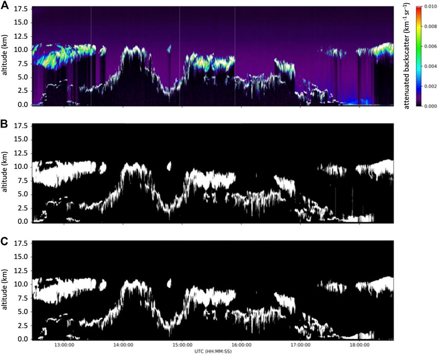
FIGURE 2. (A) CPL 532 nm attenuated backscatter profiles for 08 February 2022. (B) Result of layer detection using traditional method. (C) Result of real-time layer detection using AI/ML method.

From Figure 2 it is visually evident that the real-time algorithm is performing well compared to the traditional method. The accepted method of quantifying algorithm performance is to examine the so-called confusion matrix, or error matrix (Ting, 2011). The confusion matrix compares the AI/ML-derived result, in a supervised learning environment, to truth. In this case, because the CPL data is real and not modeled the “truth” is taken to be the results obtained via the traditional processing method. In this sense, the confusion matrix is comparing the AI/ML-derived product to the traditional product, with inherent understanding that the traditional product is itself not perfect. The confusion matrix for the data displayed in Figure 2, shown in Figure 3, shows good agreement with over 98% agreement that “no layer” data bins were properly categorized and 89% of layer-containing data bins were properly categorized. In this particular example, the largest divergence is the AI/ML method missing layers that the traditional method identifies (−10% of those data bins misclassified). That discrepancy is mostly due to the traditional method averaging over 5 s (or 50 profiles per result) whereas the AI/ML method is operating on a single profile (that is, a single subsampled 1 Hz profile per result). Thus, the traditional method is operating on profile data with inherently higher SNR. Yet, the AI/ML results are highly comparable even though using only 1/50 the signal. The performance of the AI/ML method, in real time, is comparable to traditional post-flight processing, demonstrating that the data products generated in real time are highly credible.

FIGURE 3

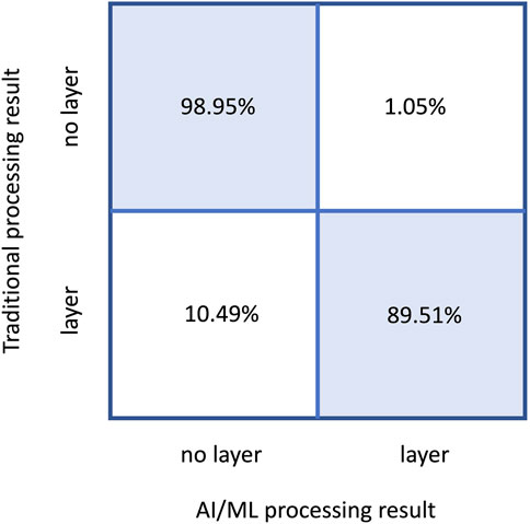
FIGURE 3. Confusion matrix for 08 February 2022 example.

To better emphasize this point, Figure 4 shows a 10-min data segment of the CPL 532 nm attenuated backscatter profiles for 08 February 2022 from near the end of Figure 2. The top panel shows the full resolution data volume, with profiles saved at 10 Hz. This is the data the traditional processing method uses when averaged to 5 s (i.e., 50 profiles are averaged together and then a layer detection is performed). The bottom panel shows the subsampled data volume, where a single 10 Hz profile is transmitted each second. This is the data the AI/ML algorithm uses, at the native resolution (i.e., no averaging of profiles). Figure 4 makes it more visually apparent that the AI/ML method is operating on noisier data and at higher horizontal resolution. Moreover, the AI/ML method is detecting layers in real time (meaning, within about one second of data collection) as each profile is received at the Jetson TX2 board.

FIGURE 4

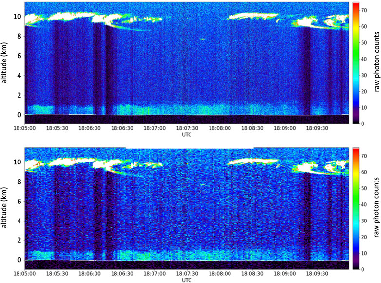
FIGURE 4. 10-min data segment from near the end of Figure 2. Top panel shows the full raw data volume, with profiles saved at 10 Hz. Bottom panel shows the subsampled data volume, where a single 10 Hz profile is transmitted each second. This is the data the AI/ML algorithm uses, at the native resolution (i.e., no averaging of profiles).

A second example, from 22 February 2022, shows similar results over a noticeably different scene. Similar to Figure 2, Figure 5 shows the CPL 532 nm attenuated backscatter profiles, the layer detection from the standard processing technique, and the layer detection result using the AI/ML technique. Note that in this example the boundary layer is evident through most of the flight, with few higher level clouds present. The confusion matrix, in Figure 6, is similar to the previous example even given the dramatically different scene type. Similar analysis over other, varying scene types provide confidence that the technique works over the range of atmospheric scenes experienced by airborne and spaceborne sensors.

FIGURE 5

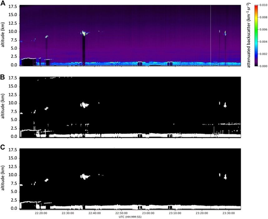
FIGURE 5. (A) CPL 532 nm attenuated backscatter profiles for 22 February 2022. (B) Result of layer detection using traditional method. (C) Result of real-time layer detection using AI/ML method.

FIGURE 6

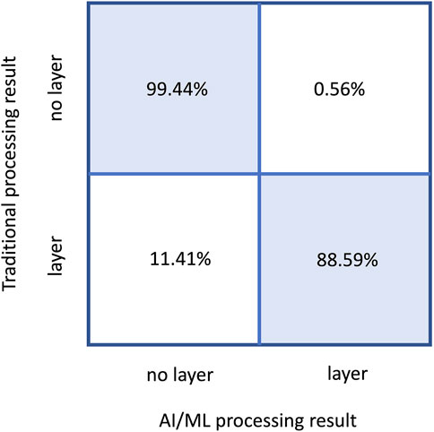
FIGURE 6. Confusion matrix for 22 February 2022 example.

4 Conclusion

In this work we apply CNN algorithms for true real-time detection of atmospheric features and determination of feature height. The real-time layer heights enabled by the technology outlined in this paper can provide information about the vertical structure of hazardous plumes and directly address critical data needs identified by forecasting agencies. Initial application and testing was accomplished using a high-altitude airborne photon-counting lidar, but the extension to spaceborne photon-counting lidar should be immediately apparent. Although spaceborne data may be more noisy compared to data from aircraft altitudes, the prior denoising work [published in (Yorks et al., 2021) using spaceborne data] demonstrates the effectiveness of the AI/ML techniques when presented with noisy data sources.

The demonstrated ability of the CNN algorithm to provide true real-time layer detection at native data resolution provides a dramatic increase in both data product availability (real time, within −1 s of data collection, as opposed to post-processed) and horizontal resolution of the feature heights (in this case, 20 m compared to 5 km). The confusion matrices that compare the CNN algorithm performance to baseline traditional processing results show >95% agreement with the thresholding techniques traditionally used to find layers, thus providing good confidence that the CNN method produces reliable real-time data products even at the higher horizontal resolution.

Although developed and tested using a high-altitude aircraft instrument, extension of the analysis techniques to spaceborne photon-counting lidar data is conceptually apparent. This is of importance for future spaceborne lidar sensors, where real-time data and data products will be essential as inputs to forecast models. Moreover, the ability to generate accurate data products at native resolution, in contrast to the normal approach of averaging multiple profiles to obtain a result, portends a sought-after increase in lidar data resolution without levying greater demands on the instrument power-aperture product. Subsequent work will focus on the next step of classifying the detected layer (i.e., as ice cloud, water cloud, smoke, dust, etc). Developing a true real time layer classification product will prove highly impactful to aerosol forecast models and real-time applications.

Data availability statement

The datasets presented in this study can be found in online repositories. The names of the repository/repositories and accession number(s) can be found below: https://cpl.gsfc.nasa.gov.

Author contributions

MM was lead (or Principal Investigator) for this work. PS led development of the AI/ML algorithms and training. AK led implementation of the hardware on the airborne sensor. JY assisted with data analysis and assembling the manuscript. All authors contributed to the article and approved the submitted version.

Funding

Funding from NASA’s Earth Science Technology Office (ESTO) enabled development and demonstration of the real-time data production capability using the CPL instrument.

Conflict of interest

Authors PS and AK are employed by Science Systems and Applications, Inc.

The remaining authors declare that the research was conducted in the absence of any commercial or financial relationships that could be construed as a potential conflict of interest.

Publisher’s note

All claims expressed in this article are solely those of the authors and do not necessarily represent those of their affiliated organizations, or those of the publisher, the editors and the reviewers. Any product that may be evaluated in this article, or claim that may be made by its manufacturer, is not guaranteed or endorsed by the publisher.

References

Benedetti, A., Reid, J. S., Knippertz, P., Marsham, J. H., Di Giuseppe, F., Remy, S., et al. (2018). Status and future of numerical atmospheric aerosol prediction with a focus on data requirements. Atmos. Chem. Phys. 18, 10615–10643. doi:10.5194/acp-18-10615-2018

CrossRef Full Text | Google Scholar

Hughes, E. J., Yorks, J. E., Krotkov, N. A., da Silva, A. M., and McGill, M. (2016). Using CATS near-realtime lidar observations to monitor and constrain volcanic sulfur dioxide (SO2) forecasts. Geophys. Res. Lett. 43 , 11089–11097. doi:10.1002/2016GL070119

CrossRef Full Text | Google Scholar

Hlavka, D. L., Yorks, J. E., Young, S. A., Vaughan, M. A., Kuehn, R. E., McGill, M. J., et al. (2012). Airborne validation of cirrus cloud properties derived from CALIPSO lidar measurements: Optical properties. J. Geophys. Res. 117, D09207. doi:10.1029/2011JD017053

CrossRef Full Text | Google Scholar

Janiskova, M., Michele, S. D., Stiller, O., Forbes, R., Morcrette, J. J., Ahlgrimm, M., et al. (2010). “QuARL: Quantitative assessment of the operational value of space-borne radar and lidar measurements of clouds and aerosol profiles,”. ESA Executive Summary Report.

Google Scholar

Kipling, Z., Stier, P., Johnson, C. E., Mann, G. W., Bellouin, N., Bauer, S. E., et al. (2016). What controls the vertical distribution of aerosol? Relationships between process sensitivity in HadGEM3–UKCA and inter-model variation from AeroCom phase II. Atmos. Chem. Phys. 16, 2221–2241. doi:10.5194/acp-16-2221-2016

CrossRef Full Text | Google Scholar

Klett, J. D. (1981). Stable analytical inversion solution for processing lidar returns. Appl. Opt. 20, 211–220. doi:10.1364/ao.20.000211

PubMed Abstract | CrossRef Full Text | Google Scholar

Krishnamurthy, R., Newsom, R. K., Berg, L. K., Xiao, H., Ma, P.-L., Turner, D. D., et al. (2021). On the estimation of boundary layer heights: a machine learning approach. Atmos. Meas. Tech. 14, 4403–4424. doi:10.5194/amt-14-4403-2021

CrossRef Full Text | Google Scholar

Marchand, R., and Ackerman, T. (2010). An analysis of cloud cover in multiscale modeling framework global climate model simulations using 4 and 1 km horizontal grids. J. Geophys. Res. 115, D16207. doi:10.1029/2009JD013423

CrossRef Full Text | Google Scholar

McGill, M. J., Hlavka, D. L., Hart, W. D., Scott, V. S., Spinhirne, J. D., and Schmid, B. (2002). Cloud Physics lidar: Instrument description and initial measurement results. Appl. Opt. 41, 3725–3734. doi:10.1364/AO.41.003725

PubMed Abstract | CrossRef Full Text | Google Scholar

McMurdie, L. A., Heymsfield, G. M., Yorks, J. E., Braun, S. A., Skofronick-Jackson, G., Rauber, R. M., et al. (2022). Chasing Snowstorms: The investigation of Microphysics and precipitation for atlantic coast-threatening Snowstorms (IMPACTS) campaign. Bull. Am. Meteorological Soc. 103, E1243–E1269. doi:10.1175/BAMS-D-20-0246.1

CrossRef Full Text | Google Scholar

Palm, S. P., Selmer, P., Yorks, J., Nicholls, S., and Nowottnick, E. (2021). Planetary Boundary Layer height estimates from ICESat-2 and CATS backscatter measurements. Front. Remote Sens. 2, 716951. doi:10.3389/frsen.2021.716951

CrossRef Full Text | Google Scholar

Ronneberger, O., Fischer, P., and Brox, T. (2015). “U-Net: Convolutional networks for biomedical image segmentation,” in International conference on medical image computing and computer-assisted intervention, proceedings of the medical image computing and computer-assisted intervention—MICCAI 2015, 18th international conference, munich, Germany, 5–9 october 2015. Lecture notes in computer science. Editors N. Navab, J. Hornegger, W. M. Wells, and A. F. Frangi (Cham, Switzerland: Springer International Publishing), 234–241.

CrossRef Full Text | Google Scholar

O’Sullivan, D., Marenco, F., Ryder, C. L., Pradhan, Y., Kipling, Z., Johnson, B., et al. (2020). Models transport Saharan dust too low in the atmosphere compared to observations. Atmos. Chem. Phys. 20, 12955–12982. doi:10.5194/acp-20-12955-2020

CrossRef Full Text | Google Scholar

Ting, K. M. (2011). “Confusion matrix,” in Encyclopedia of machine learning. Editors C. Sammut, and G. I. Webb (Boston, MA: Springer). doi:10.1007/978-0-387-30164-8_157

CrossRef Full Text | Google Scholar

Yorks, J. E., Hlavka, D. L., Vaughan, M. A., McGill, M. J., Hart, W. D., Rodier, S., et al. (2011). Airborne validation of cirrus cloud properties derived from CALIPSO lidar measurements: Spatial properties. J. Geophys. Res. 116, D19207. doi:10.1029/2011JD015942

CrossRef Full Text | Google Scholar

Yorks, J. E., Selmer, P. A., Kupchock, A., Nowottnick, E. P., Christian, K. E., Rusinek, D., et al. (2021). Aerosol and cloud detection using machine learning algorithms and space-based lidar data. Atmosphere 12, 606. doi:10.3390/atmos12050606

CrossRef Full Text | Google Scholar

Zhang, J., Campbell, J. R., Reid, J. S., Westphal, D. L., Baker, N. L., Campbell, W. F., et al. (2011). Evaluating the impact of assimilating CALIOP-derived aerosol extinction profiles on a global mass transport model. Geophys. Res. Lett. 38, L14801. doi:10.1029/2011GL047737

CrossRef Full Text | Google Scholar