Feasibility of cross-calibrating ocean-color sensors in polar orbit using an intermediary geostationary sensor of reference

A generic methodology is presented to cross-calibrate satellite ocean-color sensors in polar orbit via an intermediary geostationary sensor of reference. In this study, AHI onboard Hiwamari-8 is used as the intermediary sensor to cross-calibrate SGLI onboard GCOM-C and MODIS onboard Aqua and Terra (MODIS-A and MODIS-T) after system vicarious calibration (SVC). Numerous coincidences were obtained near the Equator using 3 days of imagery, i.e., 11 May 2018, 22 January 2019, and 25 January 2020. Spectral matching to AHI spectral bands was first performed for a wide range of angular geometry, aerosol conditions, and Case 1 waters using a single band or multiple bands of SGLI, MODIS-A and MODIS-T, yielding root mean square differences of 0.1–0.7% in the blue and green and 0.7%–3.7% in the red depending on the band combination. Limited by the inherent AHI instrument noise and the system vicarious calibration of individual polar-orbiting sensors, cross-calibration was only performed for equivalent AHI bands centered on at 471, 510, and 639 nm. Results show that MODIS-A and MODIS-T are accurately cross-calibrated, with cross-calibration ratios differing by 0.1%–0.8% in magnitude. These differences are within or slightly outside the estimated uncertainties of ±0.6% to ±1.0%. In contrast, SGLI shows larger cross-calibration differences, i.e., 1.4%, 3.4%, and 1.1% with MODIS-A and 1.5%, 4.6%, and 1.5% with MODIS-T, respectively. These differences are above uncertainties of ±0.8–1.0% at 471 and 510 nm and within uncertainties of ±2.3% and ±1.9% at 639 nm. Such differences may introduce significant discrepancies between ocean-color products generated from SGLI and MODIS data, although some compensation may occur because different atmospheric correction schemes are used to process SGLI and MODIS imagery, and SVC is based on the selected scheme. Geostationary sensors with ocean color capability have potential to improve the spectral matching and reduce uncertainties, as long as they provide imagery at sufficient cadence over equatorial regions. The methodology is applicable to polar-orbiting optical sensors in general and can be implemented operationally to ensure consistency of products generated by individual sensors in establishing long-term data records for climate studies.

1 Introduction

Accurate radiometric calibration of space-borne instruments measuring the solar radiation reflected by the Earth-atmosphere system is essential for quantitative remote sensing of land, ocean, and atmosphere properties. Radiometric calibration is performed in the laboratory before launch, but accuracy is not perfect and sometimes insufficient. In fact, this engineering calibration refers to standards (Datla et al., 2011) while science applications require a calibration with respect to solar irradiance which shows different spectral distribution. Since instruments degrade after launch due to out-gassing when the instrument leaves the atmosphere, aging of the optics, contamination of optical parts in orbit, and exposure of optical parts, detectors, and electronics to space radiation, satellite platforms are often equipped with onboard calibration devices (Kang et al., 2010; Delwart and Bourg, 2011; Okuyama et al., 2018; Xiong et al., 2020). Indirect, so-called “vicarious” methods are also used, either alternatively (in the absence of onboard calibrators) or to check the onboard device (Fougnie et al., 1999, 2007; Martiny et al., 2005; Hlaing et al., 2014; Chen et al., 2021).

Satellite ocean-color instruments have provided observations on spatial and temporal variability of the world’s oceans unattainable by conventional means, which requires very high accuracy in absolute calibration because the signal to extract is relatively small compared with the measured signal, dominated by atmospheric scattering (Gordon, 1997; Frouin et al., 2019). Atmospheric correction subtracts the atmospheric scattering signal but amplifies the relative errors on the retrieved ocean parameters due to imperfect radiometric calibration. Long-term and consistent ocean color datasets, i.e., with minimized errors/biases between different sensors, is particularly important in the context of climate studies (Sathyendranath et al., 2019). Although the “system” vicarious calibration (SVC) has traditionally been carried out for most heritage and current ocean color sensors by applying gain factors to Top-Of-Atmosphere (TOA) signals so that the remotely derived geophysical parameters fit the corresponding in situ measured parameters after atmospheric correction (Murakami et al., 2005; 2022; Franz et al., 2007; Ahn et al., 2015), biases/errors may still exist in the ocean-color products from different instruments (Djavidnia et al., 2010; Mélin, 2010; Zibordi et al., 2012; Mélin et al., 2016; Bisson et al., 2021), making it difficult to merge the data correctly and generate consistent time series.

Radiometric cross-calibration of ocean-color instruments, therefore, is an important activity to ensure product consistency and generate climate data records, all the more as many such instruments, US and foreign, have been or will be launched, on both polar orbiters, e.g., the Moderate Resolution Imaging Spectroradiometer (MODIS) onboard Aqua and Terra (hereafter referred to as MODIS-A and -T), the Medium-Resolution Imaging Spectrometer (MERIS) on the Envisat, the Visible Infrared Imaging Radiometer Suite (VIIRS) on the Suomi National Polar-orbiting Partnership (SNPP) and the Joint Polar Satellite System (JPSS) series, the Second-Generation Global Imager (SGLI) on the Global Change Observation Mission-Climate (GCOM-C) satellite, the Ocean and Land Colour Instrument (OLCI) on the Sentinel-3 series, the Ocean Color Imager (OCI) on the Phytoplankton, Aerosols, Clouds, and Ecosystems (PACE) platform, and geostationary satellites, e.g., the Geostationary Ocean Color Imager (GOCI), GOCI-II, the and the Geosynchronous Littoral Imaging and Monitoring Radiometer (GLIMR). A better merging of the geophysical ocean-color products would obviously require processing all the Level-1 data with the same algorithm applied to different sensors that have been cross-calibrated, meaning with a common reference to the same absolute radiometric calibration.

Radiometric cross-calibration can be easily defined as viewing the same radiance at the same time, but it is much more difficult to achieve during in flight operations of different sensors on different orbits. Apart from viewing the Moon, one must rely on measuring the solar radiation reflected by the Earth-atmosphere system at the same time and location because of its time variability. Moreover, the Earth-atmosphere system may have some bidirectional reflectance function that requires observing under the same solar and viewing geometry. At last, if the spectral bands of the channels to be compared do not have the same or close definition, some empirical transformations must be applied to make the comparison thus the cross-calibration.

Bright surfaces, mostly arid deserts like White Sands and the Sahara Desert have been used to calibrate, thus possibly cross-calibrate satellite sensors for land surface remote sensing with some success (Lacherade et al., 2013). The methodology assumes that the variations of the bidirectional reflectance of the surface with the viewing and solar geometry is accurately known and that the atmosphere has a minimum influence. Moon calibration is about the same technique with the advantage of no atmosphere interference but requires some maneuvers of the polar orbiting platform to view the Moon (Eplee et al., 2011). Cao et al. (2004) suggested cross calibrating the sensors over the polar regions by taking advantages of the multiple passes of a polar orbiting platform at high latitude. This allows one to better solve the requirements on geometry and simultaneity.

Ocean (and aerosols over the ocean) remote sensing, however, deals with a lower dynamic of the radiometry than over the land surface. Therefore, one cannot use the highly reflecting “stable” targets of the desert and polar caps because of possible linearity and saturation problems of ocean-color sensors. Ocean targets used with some successes are waters at instrumented buoys like MOBY and BOUSSOLE (Clark et al., 1997; Antoine et al., 2006; Antoine et al., 2008) and the “stable” waters in the center of the subtropical gyres (Hagolle et al., 1999). But most of the TOA radiance is dominated by atmospheric scattering. More generally the measured signal, mostly atmospheric, changes strongly with geometry through atmospheric scattering and with time through aerosol/sub-cloud variability. The SVC method does not explicitly solve the problem and is only performed in the visible. The near-infrared bands remain un-calibrated and may lead to overall systematic biases. For example, about 3%–3.5% differences have been identified between MODIS-A and VIIRS/SNPP in the long near infrared bands (Sayer et al., 2017; Barnes et al., 2021) and such differences at this wavelength partly contribute to the cross-sensor biases of downstream geophysical products (Barnes et al., 2021).

Viewing the same location by two polar-orbiting sensors at the same time and with the same geometry is not an easy task. In-flight comparison between polar-orbiting sensors is limited by the requirements for simultaneously viewing a location with the same geometry. The probability of such event for sensors onboard platforms having different equatorial crossing times increases with latitude. It is nevertheless not very frequent over the polar region, see Cao et al. (2004). An alternative way is to consider the viewing and illumination geometries and then simulate the expected TOA radiances using the water-leaving radiances from other sensors so that more match-up data are available for cross-calibration, as is done for MODIS-T (Kwiatkowska et al., 2008; Meister and Franz, 2011). Inter-calibrating two different geostationary sensors is even more difficult or unfeasible when their sub-satellite points are far away on the Equator.

This study utilizes a geostationary sensor, i.e., the Advanced Himawari Imager (AHI) on board Himawari-8, to cross-calibrate satellite ocean color sensors in polar orbits, i.e., MODIS-A, MODIS-T, and SGLI onboard GCOM-C. The geostationary sensor can be viewed as a robin between polar-orbiting sensors. This is facilitated by the frequent time and geometry coincidences, about daily, when the polar-orbiting sensor crosses the field-of-view of the geostationary sensor around the Equator. In previous studies, AHI onboard Himawari has been utilized to cross-calibrate the solar reflective bands of VIIRS and MODIS (Yu and Wu, 2016; Qin et al., 2018) and the thermal emissive bands of MODIS-A and MODIS-T (Chang et al., 2019), although the calibrations are not ocean specific. Murakami et al. (2019) did some preliminary work on cross-calibrating SGLI, MODIS-A, and VIIRS with AHI over global oceans using modeled bidirectional reflectance distribution function (BRDF) and aerosol signals. However, none of these studies attempted to use AHI to cross-calibrate polar-orbiting sensors. In Section 2, a brief description of the different satellite sensors is provided, including both the spectral and spatial characteristics as well as data access. In Section 3, the generic methodology and algorithm for the cross-calibration of polar-orbiting sensors is presented. The procedure consists of cross-calibrating separately the polar-orbiting sensors against the geostationary sensor of reference. This requires spectral matching the bands of the polar-orbiting sensors to equivalent reference bands and finding coincidences between observations by the polar-orbiting sensors and the geostationary sensor of reference. In Section 4 and Section 5, the results of spectral band matching, coincident pixels selection, and cross-calibration (first for individual polar-orbiting sensor separately with respect to the geostationary sensor, then between polar-orbiting sensor pairs) are shown. The uncertainties on the cross-calibration coefficients at various bands are also estimated. In Section 6, finally, the cross-calibrating method and results obtained for SGLI, MODIS-A, and MODIS-T are summarized. Advantages and limitations are discussed, as well as the potential of using new and future geostationary sensors.

2 Satellite sensors

2.1 AHI

AHI is carried by the Japanese geostationary weather satellite Himawari-8, which was successfully launched on 7 October 2014 and has been operational since July 2015. It views the Earth at an altitude of approximately 35,800 km and is configured to scan the full disk (centered at 0° N, 140.7° E) every 10 min. During this interval, AHI also scans Japan Areas and a selectable Target Area 4 times and two Landmark Areas (for navigation use only) 20 times. The AHI has a total of 16 multispectral bands, including six visible and near infrared (VNIR) bands and 10 thermal emissive bands. The spatial resolution of the six VNIR bands varies from 0.5 km to 2 km, i.e., 1 km resolution for band 1 (470 nm), 2 (510 nm), and 4 (857 nm), 0.5 km for band 3 (639 nm), and 2 km for band 5 (1,610 nm) and 6 (2,257 nm). Level-1 gridded AHI data, which has been resampled into 5-km and 2-km equal latitude-longitude grids, is generated by Japan Aerospace Exploration Agency Earth Observation Research Center (JAXA EORC) from the Himawari Standard Data and is distributed via JAXA’s P-Tree system (https://www.eorc.jaxa.jp/index.html). On-orbit calibration of the AHI data is performed using an internal blackbody target and deep space for infrared bands and using the solar diffuser and deep space observations for the VNIR bands, the latter performed twice a month (Okuyama et al., 2018). The AHI does not carry equipment to monitor solar diffuser degradation. Nevertheless, the AHI calibration coefficients from solar diffuser observation are updated every July and the temporal drift has been adjusted in the level-1 data (JMA, 2017). In addition, radiometric calibration of the AHI VNIR bands is examined by comparing the measured radiance with simulated radiance from radiative transfer calculations with satellite observed atmospheric and geometric conditions as input (https://www.data.jma.go.jp/mscweb/data/monitoring/gsics/vis/techinfo_visvical.html). In this study, only the 2-km full disk level-1 data are used, from which TOA reflectance can be obtained directly by dividing the provided albedo by the cosine of solar zenith angle. Level-2 cloud property data (only available at 5-km resolution) that are also produced and archived by JAXA are used to generate cloud mask for screening out cloudy pixels, as described in the following Section 5.

2.2 MODIS

MODIS is operating on both the Terra and Aqua satellites, which were successfully launched on 18 December 1999, and 4 May 2002, respectively. The local Equator crossing time for Terra at ascending node is ∼10:30 am and Aqua ∼1:30 p.m. MODIS has 36 spectral bands ranging from 0.4 to 14.4 µm and views the Earth with a wide swath of 2,300 km and a 1–2 day repeat cycle of data collection. There are 9 bands in the VNIR range from 412 to 869 nm that are specifically designed for ocean color observation and the spatial resolution is approximately 1 km at nadir. Other bands on MODIS are designed for land and cloud observations. They overlap the spectral range of the ocean bands and extend into short-wave infrared (SWIR), from 469 to 2,130 nm, with increased spatial resolution, i.e., 250–500-m at nadir. Ocean color observations from MODIS-A and -T have been routinely made available by the National Aeronautics and Space Administration Ocean Biology Processing Group (NASA OBPG) over two decades. Both MODIS-A and MODIS-T instruments are calibrated using onboard calibrators (Xiong et al., 2019) and lunar irradiances (Sun et al., 2007). Such calibrations have been sufficient to produce high quality ocean color products up to 2007 for MODIS-A, but not for MODIS-T, which requires an additional on-orbit cross-calibration approach that derives the expected TOA radiance field using water-leaving radiances from other sensors (e.g., Sea-viewing Wide Field-of-view Sensor, SeaWiFS, Kwiatkowska et al., 2008) and MODIS-T viewing and illumination geometries. For ocean color purposes SVC is also applied according to Franz et al. (2007). Level-1a MODIS-A and -T data are available from the OBPG website (https://oceancolor.gsfc.nasa.gov) in both VNIR and SWIR bands (including ocean, land, and cloud bands). The SeaWiFS Data Analysis System (SeaDAS, https://seadas.gsfc.nasa.gov) software is used to generate level-1b product which contains TOA reflectance from level-1a sensor counts at a spatial resolution of 1 km for wavelengths 412, 443, 469, 488, 531, 547, 555, 645, 667, 678, 748, 859, 869, 1,240, 1,640, and 2,130 nm. Note that vicarious calibration gains are applied during the conversion, which means the level-1b TOA reflectance is the one after SVC.

2.3 SGLI

Launched on 23 December 2017, the JAXA polar-orbit satellite GCOM-C carries SGLI, which has 19 channels in the wavelength range from near-UV to thermal infrared (380 nm–12 um) with resolutions of 250 m to 1 km, including 11 non-polarized VNIR channels (380, 412, 443, 530, 566, 672, 763, and 867 nm), 2 polarization channels centered on red and near-infrared wavelengths of 670 and 870 nm, 4 channels in the SWIR (1,050, 1,380, 1,635, and 2,209 nm), and 2 channels in the thermal infrared (TIR). There are two bands centered at 672 nm and at 867 nm, but only those with higher Signal-to-Noise ratio (SNR) are used for ocean color purposes. SGLI collects observation data of the entire Earth every 2 or 3 days. The swath width of SGLI is 1,150 km for the VNIR channels and 1,400 km for all the SWIR and TIR channels. Onboard radiometric calibration of SGLI VNIR bands is performed using an internal lamp and a solar diffuser (Okamura et al., 2018; Tanaka et al., 2018; Urabe et al., 2020). The GCOM-C satellite is also designed for lunar calibration maneuver to check the stability of SGLI calibration (Urabe et al., 2019). The temporal drift has been considered in the radiometric calibration of the TOA radiance. The SGLI data is archived at JAXA’s G-Portal (https://gportal.jaxa.jp/gpr/). Both 250 m and 1 km (resampled) level-1b are provided, but only 1-km data is used in the analyses. Like MODIS, SGLI level-1b data is vicariously calibrated, using the detailed procedure described in Murakami et al. (2022).

3 Methodology

Cross-calibration of satellite instruments is a process or operation that relates the detector output of a sensor in a spectral band to the detector output of another sensor in a similar spectral band. The procedure requires that the observations by the two instruments are collocated in space and time and that the respective viewing zenith and azimuth angles are close. This is not easy to achieve when the two instruments are on different polar orbits, as indicated in Section 1, which is the case for global ocean-color sensors. To increase the number of coincidences, this study utilizes a sensor in geostationary altitude as an intermediary or robin, against which the sensors to cross-calibrate are matched.

Consider the cross-calibration of two polar-orbiting sensors. Denote by ${\rho }_{1i}\left(t\right)$ and ${\rho }_{2j}\left(t^{\prime }\right)$ the reflectance measured at time $t$ by the first sensor and $t^{\prime }$ by the second sensor in spectral bands $i$ and $j$, respectively, and by ${\rho }_{ref}\left(t\right)$ and ${\rho }_{ref}\left(t^{\prime }\right)$ the reflectance measured at $t$ and $t^{\prime }$ by the geostationary sensor in a spectral band of reference. It is assumed here, for simplicity, that the polar-orbiting and geostationary sensors observe at the same time. Differences in observation time, generally small, will be accounted for in application. The cross-calibration coefficients between each polar-orbiting sensor and the geostationary sensor, $A_{1i}$ and $A_{2j}$, can be written as:

$A_{1i}={\rho }_{ref}\left(t\right)/f_{1i}\left[{\rho }_{1i}\left(t\right)\right](1)$

$A_{2j}={\rho }_{ref}\left(t^{\prime }\right)/f_{2j}\left[{\rho }_{2j}\left(t^{\prime }\right)\right](2)$

where $f_{1i}$ and $f_{2j}$ are empirical functions that relate ${\rho }_{1i}$ and ${\rho }_{2j}$ to ${\rho }_{ref}$. These functions are determined theoretically, from simulations for realistic environment and geometry conditions. If the two sensors are perfectly inter-calibrated, $A_{1i}$ is equal to $A_{2j}$. Differences between $A_{1i}$ and $A_{2j}$, on the other hand, will indicate that the calibration of the two sensors is not consistent and, therefore, needs to be adjusted accordingly. It is assumed, indeed, that the three sensors involved do not exhibit degradation or other changes between $t$ and $t^{\prime }$. The difference between these times, however, is expected to be small, i.e., a few hours.

Note that depending on the spectral band, the ${\rho }_{ref}$ measurements may not be well correlated to ${\rho }_1$ and ${\rho }_2$ measurements in a single spectral band, but to measurements in several spectral bands. For example, the blue band of AHI is relatively large (with bandwidth of 50 nm) and can only be accurately represented using two spectral bands of SGLI (see Section 4). The formalism remains the same, but Eqs 1, 2 become:

$A_{1M}={\rho }_{ref}\left(t\right)/f_{1M}\left[{\rho }_{1i}\left(t\right),i=1,2,\dots ,M\right](3)$

$A_{2N}={\rho }_{ref}\left(t^{\prime }\right)/f_{2N}\left[{\rho }_{2j}\left(t^{\prime }\right),j=1,2,\dots ,N\right](4)$

where the empirical functions $f_{1M}$ and $f_{2N}$ now relate ${\rho }_{ref}$ to a combination of measurements ${\rho }_{1i}$ in $M$ spectral bands and ${\rho }_{2j}$ in $N$ spectral bands. Consequently, differences between $A_{1M}$ and $A_{2N}$ will only be indicative of calibration inconsistencies in combination of spectral bands, not single bands. If not complete, this information is useful, and $A_{1M}$ should be equal to $A_{2N}$ in any calibration normalization.

4 Spectral band matching

Since the spectral bands of the sensors to cross-calibrate and the geostationary sensor, i.e., AHI/SGLI, AHI/MODIS-A, and AHI/MODIS-T, do not match exactly, it is essential to perform spectral matching before any further analyses. The accuracy of cross-calibration depends on how well SGLI, MODIS-A and -T data can be transformed into equivalent AHI data. Figure 1 displays the normalized spectral response of AHI, MODIS-A, MODIS-T, and SGLI bands. Only the bands that have overlap with other sensors are shown. It is clear that there are differences between the sensors except that MODIS-A and MODIS-T have almost identical relative spectral responses. The SGLI and MODIS bands are available in the proximity of, if not within, almost each of the AHI bands. Both SGLI and MODIS are spectrally similar at 443, 490, 530, and 867 nm. Unfortunately, there is no such well-matched SGLI or MODIS spectral response for AHI bands except for MODIS at 859 nm. The AHI bands generally have relatively large bandwidth and/or are not centered on the same (or similar) wavelength as SGLI and MODIS. Due to these differences, it would be difficult to directly pair one SGLI or MODIS band with one AHI band for some cases. Instead, multiple SGLI or MODIS bands may be combined.

FIGURE 1

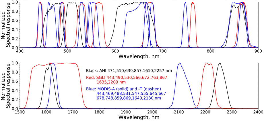
FIGURE 1. Normalized spectral response of AHI (black), SGLI (red), MODIS-A (blue solid), and MODIS-T (blue dashed) bands.

Matching the AHI reflectance was achieved as follows. If the spectral band of the polar-orbiting sensor is either centered on about the same wavelength or has similar bandwidths as the band of the geostationary sensor, their reflectance, ${\rho }_{GEO}$ and ${\rho }_{LEO}$ (subscripts $GEO$ and $LEO$ representing the geostationary and polar-orbiting, or Low Earth Orbiting sensors, respectively), are related by a simple linear fit, i.e., ${\rho }_{GEO}=C_0+C{\rho }_{LEO}$. If the spectral band of the geostationary sensor is large, one needs to compute its reflectance by combining reflectance in several spectral bands $i$ of the polar-orbiting sensor, i.e., ${\rho }_{GEO}=C_0+{\displaystyle \sum }_i{C}_i{\rho }_{LE{O}_i}$.

Radiative transfer simulations using the Second Simulation of a Satellite Signal in the Solar Spectrum Vector (6SV) code (Kotchenova et al., 2006; Kotchenova and Vermote, 2007) were used to simulate ${\rho }_{GEO}$ and ${\rho }_{LEO}$ for a wide range of aerosols and marine reflectance conditions. The TOA reflectance was computed at SGLI and MODIS (Aqua and Terra separately) wavelengths, for total aerosol optical thickness values ranging from 0.1 to 0.3 at 550 nm. Maritime, continental, and urban aerosol models were considered. Simulations were carried out for Sun zenith angles (SZA) ranging from 0° to 60°, view zenith angles (VZA) from 0° to 45°, and relative azimuth angles from 0° to 180°. Only conditions with minimum glint, i.e., with glint reflectance less than 0.05, were selected. Gaseous absorption was considered and varied in the simulations, i.e., water vapor ranging from 0 to 5 g/cm² and ozone from 0.1 to 0.35 cm-atm. Wind speed was assumed constant, i.e., 5 m/s, as the impact of wind speed is negligible when Sun glint is minimal, and chlorophyll concentrations were set to vary from 0.1 to 10.0 mg/m³ to specify different marine reflectance (Figure 8 of Morel and Maritorena, 2001). Only Case 1 waters were considered to avoid the high variability of coastal turbid waters, i.e., the matching corresponds to situations encountered in open waters, where the coincidences will be selected. Considering that correcting for gaseous absorption using ancillary ozone and water vapor data may be necessary in some cases to achieve sufficient accuracy in the spectral matching, the coefficients of the linear and multi-linear regressions were obtained with and without gaseous absorption.

Table 1 lists the combinations of SGLI, MODIS-A, and MODIS-T bands used to generate each of the equivalent AHI bands. The goal is to make sure the spectral band conversion from the polar-orbiting sensors to AHI is sufficiently accurate with the smallest number of polar-orbiting bands as possible. In the spectral matching, two sets of geometries, i.e., (VZA ≤30°, SZA ≤30°), and (VZA ≤45°, SZA ≤60°), with and without gaseous absorption, were tested. The accuracy of spectrum matching is generally higher when using reduced geometry (results not shown), i.e., VZA ≤30° and SZA ≤30°, which is expected since small differences in the optical properties of the aerosols and gas absorbers in different spectral bands are amplified when VZA and SZA are large (i.e., large air mass). The effect of gaseous absorption does not significantly degrade the quality of the spectral matching for AHI at 471 nm, 510 nm, and 639 nm, but this is the not the case when matching other pairs of bands, for example, AHI at 2,257 nm with SGLI at 2,209 nm. This is due to water vapor absorption that mainly occurs in the near- and short-wave infrared and varies significantly for different spectral bands. In matching those bands, correcting first the TOA reflectance for gaseous absorption may reduce the RMS difference by a factor of 2–8. Considering that the reduced geometry may not be applicable to satellite imagery, spectral matching using (VZA ≤45°, SZA ≤60°) and without gaseous absorption was adopted.

TABLE 1

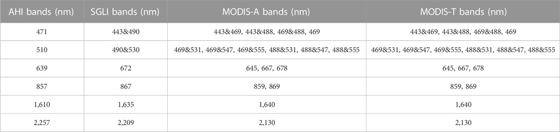
TABLE 1. A list of the combinations of SGLI, MODIS-A, and -T bands used for estimating reflectance in AHI bands.

The TOA reflectance in each AHI band can be accurately reconstructed using a single band or two bands of the polar-orbiting sensors via linear regression (Table 2). Since MODIS-A and MODIS-T have almost the same spectral response functions, it is no surprising that the relations of converting MODIS bands to AHI bands as well as the achieved root mean square difference (RMSD) are similar. As shown in Table 2, the largest RMSD is found for AHI 639 nm, which can be up to 0.00252 (3.7%) and 0.00255 (3.7%) when reconstructed using the MODIS-A and -T reflectance at 678 nm. This is probably due to AHI at 639 nm having a much larger bandwidth and MODIS at 678 nm being located near the edge of this AHI band (Figure 1). The RMSD is slightly smaller when using SGLI at 672 nm, and MODIS-A and -T at 667 nm, i.e., 0.00221 (3.2%), 0.00190 (2.8%), and 0.00194 (2.8%), respectively, and even smaller when using MODIS-A and -T at 645 nm (RMSD of 0.9% and 0.7%, respectively), as these wavelengths are closer to the center of the referenced AHI band. Similarly, the transformation from MODIS-A and -T at 2,130 nm to equivalent AHI at 2,257 nm shows a relatively large RMSD, i.e., 0.00058 (2.5%), but the spectral matching using SGLI at 2,209 nm is more accurate, i.e., 0.00017 (0.7%). In general, except for the wavelengths mentioned above, the RMSD of spectral matching are quite small, i.e., less than 0.7%. Note that accurate estimation of the reflectance at AHI wavelengths of 471 and 510 nm requires combinations of two bands and multi-linear regression in some cases. Take AHI(471) and SGLI(443) for example, the TOA reflectance is well correlated via linear regression, to a RMSD of 0.00227 (1.7%) (results not shown). A much better spectral matching is obtained, however, when the TOA reflectance in AHI(471) is regressed against the two SGLI bands at 443 and 490 nm, which gives a RMSD of 0.00052 (0.4%). The linear relations between bands of polar-orbiting sensors and AHI bands were then applied to the satellite measurements, from which the effect of gaseous absorption was beforehand removed (see Section 5).

TABLE 2

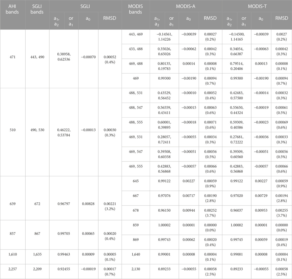
TABLE 2. The relations and corresponding RMSD for SGLI, MODIS-A, and -T band combinations to generate equivalent AHI bands, obtained using 6SV simulations with VZA ≤45°, SZA ≤60°, and no gaseous absorption (see main text for more details). TOA reflectance (denoted as ρ) at each AHI band can be generated using a₀+a₁*ρ_s,i + a₂*ρ_s,j or a₀+a₁*ρ_s,i, where subscript s represents SGLI, MODIS-A, or MODIS-T, and i, j represents band i and j.

5 Cross-calibration results

5.1 Geometry coincidence

The collocated pixels from the pairs of instruments, i.e., AHI/SGLI, AHI/MODIS-A, and AHI/MODIS-T, were selected based on the following criteria:

• Observations must be taken under comparable conditions, which means close solar and viewing angles. Only pixels within 1° for the solar zenith angle, the viewing zenith angle, the relative azimuth angle, and the scattering angle are considered.

• The time difference between the polar-orbiting and geostationary observations must be sufficiently small to neglect changes in the reflectance characteristics of the atmosphere and target. AHI images closest in time to the SGLI, MODIS-A and -T images are used, i.e., the time difference is no more than 10 min, the temporal resolution of AHI observations.

• The coincident observations should be selected preferentially over the ocean in clear sky conditions and outside the Sun glint region since ocean-color products are generated under those conditions. When clear sky images are not available, adjacency effects should be reduced, which is accomplished by avoiding pixels within a 3 × 3 window of identified cloudy pixels. Outliers are further removed by excluding pixel values that are more than two standard deviations from the mean.

To find the collocated pixels, the AHI images were first remapped to the SGLI and MODIS latitude-longitude grids using the nearest neighbor method. Since the sensors to cross-calibrate are in a strongly inclined (i.e., near polar) orbit, observations along the same line of sight by the polar-orbiting and geostationary sensors are expected to occur in a relatively small region near the equator (Western Equatorial Pacific), the only region where the viewing azimuth angles would match. Three different dates were selected (Table 3), i.e., 11 May 2018, 22 January 2019, and 25 January 2020, when relatively large areas of clear sky pixels rather than sporadic pixels between clouds were found. But this is not a necessary condition; there are many days with suitable clear pixels during the year. Such coincident pixels of all three sensors are not available on every date (Table 3). For example, only AHI/SGLI and AHI/MODIS-T have coincident pixels on 22 January 2019.

TABLE 3

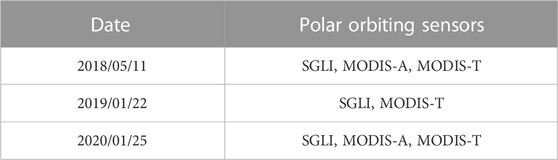
TABLE 3. A list of dates with polar orbiting sensors used in this study.

Figures 2, 3 display the AHI images and the corresponding SGLI and MODIS images acquired on 25 January 2020, for 471 nm and 639 nm, respectively. The equivalent AHI reflectance at 471 nm and 639 nm were converted using band combinations listed in Table 2, i.e., SGLI at 443 and 490 nm, MODIS-A and -T at 443 and 488 nm for AHI 471 nm, and SGLI at 672 nm, MODIS-A and -T at 667 nm for AHI at 639 nm. As indicated in Table 2, several combinations are possible; those listed above were selected as examples. The TOA reflectance is spread in the range of 0.09–0.11 and 0.025–0.05, respectively, for 471 and 639 nm, which is the typical TOA reflectance range observed over oligotrophic waters. The AHI/SGLI and AHI/MODIS-A comparisons display a larger scatter when compared to AHI/MODIS-T, probably due partly to the relatively larger fraction of coincidences in proximity of clouds. A gaseous absorption correction was first applied to the TOA reflectance using MERRA-2 (Gelaro et al., 2017) ozone and water vapor amounts obtained the same day and NO₂ amount from monthly climatology based on Aura OMI data. Note that SVC had been applied to the L1b TOA reflectance generated by the satellite project offices, i.e., we are dealing with the L1b data used to derive water reflectance via operational atmospheric correction schemes. Red rectangles show where the geometry coincidence occur if SGLI and MODIS pixels have correspondence in AHI imagery. Most of the coincident pixels in those rectangles occur under clear sky conditions, and the pixels that might be contaminated by clouds were removed using the cloud masks. The spatial features inside the rectangles are similar, but not outside the rectangles, which is expected because of the observation geometry difference. The high reflectance observed in the coastal regions located in the left part of the MODIS-A image, in particular, is due to Sun glint. The coincidences occur at different locations, which is desirable because the calibration scheme is supposed to work for all ocean conditions.

FIGURE 2

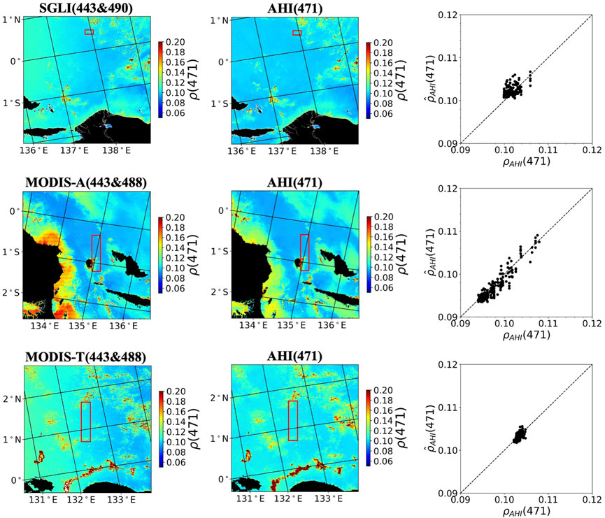
FIGURE 2. Concomitant SGLI/AHI (01:10 GMT, top row), MODIS-A/AHI (04:30 GMT, middle row), and MODIS-T/AHI (01:30 GMT, bottom row) images of TOA reflectance for 25 January 2020. The Level 1b SGLI, AHI, and MODIS data used to generate these images were downloaded from JAXA’s P-Tree system (https://www.eorc.jaxs.jp/ptree/index.html) and G-Portal (https://gportal.jaxa.jp/gpr/), and from NASA's OBPG (https://oceancolor.gsfc.nasa.gov), respectively. The AHI imagery of 471 nm was remapped to the SGLI and MODIS latitude-longitude grid, and SGLI at 443 and 490 nm and MODIS-A and -T at 443 and 488 nm were used to generate the equivalent (i.e., ${\widehat{\rho }}_{AHI}$) AHI image at 471 nm (see Table 2 for the specific coefficients to convert polar orbiter reflectance to ${\widehat{\rho }}_{AHI}$). Red rectangles indicate where the coincident pixels occur. Land is masked as black. White indicates saturated pixels. The right panel show the scatter plots of equivalent versus measured AHI reflectance.

FIGURE 3

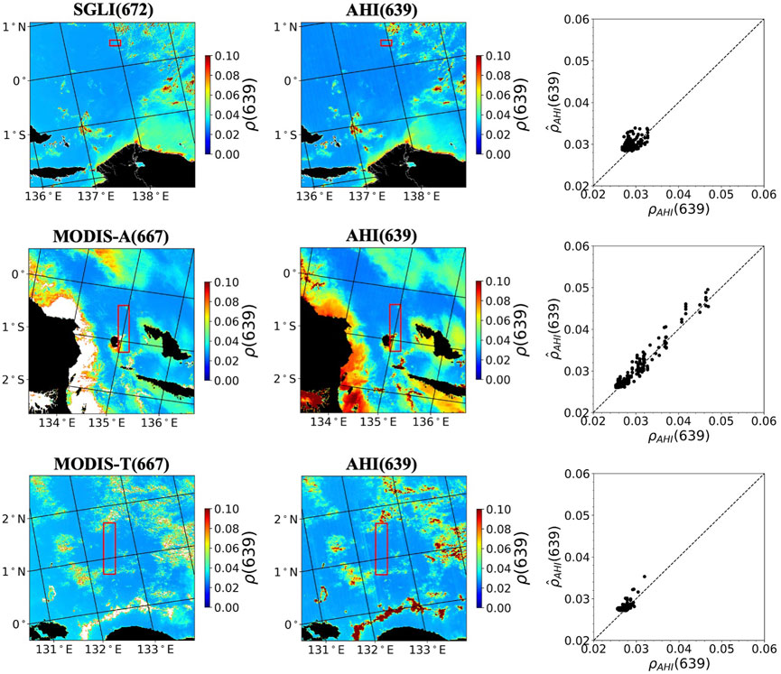
FIGURE 3. Same as Figure 2, but for AHI 639 nm. The equivalent AHI reflectance at 639 nm is obtained from SGLI reflectance at 672 nm and MODIS reflectance at 667 nm (see Table 2 for the conversion coefficients).

The coincident pixels are typically found near the Equator, and the number of pixels is numerous, 225 for AHI/SGLI, 619 for AHI/MODIS-T, and 381 for AHI/MODIS-A, respectively (Figure 4). Specifically, the AHI/SGLI coincidences (at GMT 01:10 h) are located between 0.3° and 0.6° N for solar zenith angles between 32.7° and 33.0°, viewing zenith angles between 2.5° and 4.4°, relative azimuth angles between 29.2° and 29.5°, and an average scattering angle of about 150°. The AHI/MODIS-T coincidences (at GMT 01:30 h) are located between 0.5° and 2° N, for solar zenith angles between 32.5 and 33.2°, viewing zenith angles between 8.5° and 10.9°, relative azimuth angles between 28.6° and 33.3°, and an average scattering angle of about 155°. The AHI/MODIS-A coincidences (at GMT 04:30 h) are located between 0° and 1.5° S, for solar zenith angles between 26.8 and 27.4°, viewing zenith angles between 5.8° and 7.9°, relative azimuth angles between 139.7° and 149.1° and an average scattering angle of about 147°. Combining the other two dates, the coincident pixels are observed between 1.5° S and 3° N, 126.7° E to 138.1° E, and the solar zenith angle ranges from 26.8° to 35.8°, view zenith from 2.5° to 17.6°, relative azimuth angles from 28.6 to 149.1°, and scattering angle from 146.3° to 158.8°, with at least 775 pixels per sensor pair (Table 4).

FIGURE 4

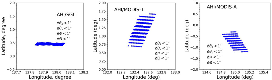
FIGURE 4. Location of clear sky AHI/SGLI (01:10 GMT, 225 pixels in total, left), AHI/MODIS-A (04:30 GMT, 381 pixels in total, middle), and AHI/MODIS-T (01:30 GMT, 619 pixels in total, right) coincidences for 25 January 2020, i.e., differences in solar zenith ($∆{\theta }_{\mathrm{s}}$), view zenith ($∆{\theta }_{\mathrm{v}}$), relative azimuth ($∆\varphi$), and scattering angle ($∆\Theta$) are less than 1°.

TABLE 4

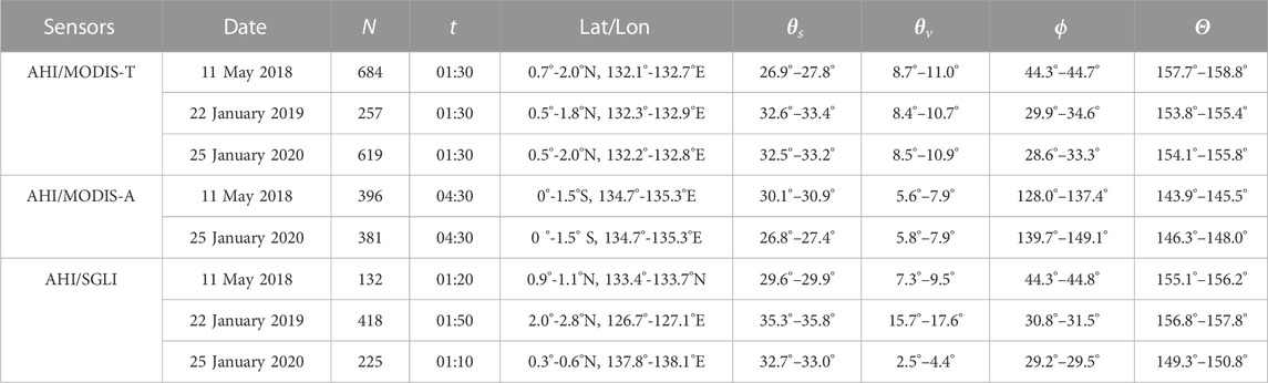
TABLE 4. The observation time (t, GMT), geometry (solar zenith ${\theta }_s$, view zenith ${\theta }_v$, relative azimuth $\varphi$, and scattering angle $\Theta$), latitude/longitude, and total number of collocated pixels N) for each sensor pair on the three different dates.

Semi-variograms (or structure functions) of the TOA reflectance were computed empirically to determine the image noises, using the equation below:

$SV\left(h\right)=\frac{1}{2N\left(h\right)}\sum \sum {\left[{\rho }_{toa}\left(M\right)-{\rho }_{toa}\left(M+h\right)\right]}^2(5)$

where ${\rho }_{toa}$ is the TOA reflectance after gaseous absorption, $M$ denotes a pixel in the image, $h$ the distance to $M$, $N$ is the number of data pairs (depends on $h$), and the double sum is over the 2-dimensional spatial field (i.e., the image). Homogeneous ocean areas from the individual images shown in Figures 2, 3 were selected to compute $SV\left(h\right)$. The $SV$ value at distance 0, i.e., $SV\left(h=0\right)$, is the unresolved variance, the square root of which represents image noise (Atkinson et al., 2007; Glover et al., 2018). To derive $SV\left(h=0\right)$, a spherical model (Cressie, 1993; Chiles and Delfiner, 1999) was used to fit the computed empirical values. The spherical model is:

$SV\left(h\right)=C_0+C\left(\frac{3h}{2d}-\frac{h^3}{2d^3}\right),if0<h\le d;SV\left(h\right)=C_0+C,ifh>d(6)$

where $C_0$ represents the unresolved variance, $C_0+C$, i.e., the total variance, and $d$ the de-correlation length scale. Results show that the AHI image has higher noise level than the SGLI and MODIS images, i.e., with higher $SV\left(h=0\right)$, which is expected because AHI is a weather satellite and not designed specifically for ocean observations. Stripe noise can also be seen in AHI images (Figure 3, middle panel). As wavelength increases, the noise become larger while the TOA reflectance decreases. For example, at 639 nm, the average TOA reflectance is about 0.03, and the $SV\left(h=0\right)$ (i.e., $C_0$) values for SGLI and AHI are about 3 × 10⁻⁸ and 5 × 10⁻⁸, respectively, which means the image noise is about 2 × 10⁻⁴, i.e., 0.6%. At longer wavelengths, i.e., 857, 1,610, and 2,257 nm, however, the AHI image noise increases to more than 3%, which will eventually propagate to the cross-calibration coefficients. Consequently, even with very accurate spectral band matching (for example, at 857 and 1,610 nm, see Table 2), these longer wavelengths are not of interest in this study, even more as for ocean color applications the SVC (Franz et al., 2007; Murakami et al., 2022) makes assumptions about radiometric calibration in the near infrared and does not consider SWIR measurements (only bands in the visible are adjusted for calibration). We keep 639 nm as the spectral matching RMSD is less than 3% for some SGLI/MODIS band combinations (Table 2).

5.2 Cross-calibration coefficients and associated uncertainties

From the collocated pixels the cross-calibration coefficient is simply calculated as the ratio of the TOA reflectance measured by the two sensors after correction for gaseous absorption (see Section 3). Remember that the goal of this study is to cross-calibrate SGLI, MODIS-A, and MODIS-T, and AHI is only used as an intermediary. Therefore, the cross-calibration coefficients of two polar-orbiting sensors should be calculated by first computing the reflectance ratio of geostationary AHI and individual polar-orbiting sensors separately and then the ratio of the resulting individual ratios. The former is performed for each of the coincident pixels per day, resulting in cross-calibrations coefficients of each day for the estimation of the latter (more details are provided below). Note that the cross-calibration coefficients obtained during a day over a target region are samples of the population of cross-calibration coefficients. This population is not negligible due to uncertainties in the radiometric calibration of individual sensors. The variance of those samples does not necessarily represent the variance of the entire population, and this needs to be considered when associating uncertainties to the estimated cross-calibration coefficients. One expects the sample variance to be closer to the population variance with an increased number of days, and the uncertainty on the cross-calibration coefficient for each sample reduced with an increased number of coincidences.

5.2.1 Pairs of AHI and polar-orbiting sensor

Figures 5, 6, 7 display the scatter plots of reflectance ratios versus solar zenith angle and histograms of reflectance ratios obtained for AHI/SGLI, AHI/MODIS-A, and AHI/MODIS-T at 471, 510, and 639 nm. The means and standard deviations of the reflectance ratios are calculated. The results show that the reflectance ratios have no obvious dependence on solar zenith angle. The standard deviations increase as the wavelength increases, which is consistent with the increasing variabilities displayed in the figures. The histograms of multiple days’ data suggest that the cross-calibration coefficients from different days are different from each other, especially at 639 nm. The underlying assumption is that the cross-calibration coefficients are identical if obtained within the same day (hence the variations are purely due to measurement errors) but may be different for different days, especially if those days are far apart, due to uncertainties in their determination (time drift may not per perfectly corrected, for example). Therefore, it is not surprising that the cross-calibration coefficients are not the same for different days. It also highlights the importance of acquiring coincidences on as many days as possible to fully characterize the distribution of cross-calibration coefficients and accurately associate uncertainties to those coefficients. Unfortunately, we do not have enough days to describe properly the population of cross-calibration coefficients for AHI and polar-orbiting sensors. Estimating the population variance based on uncertainties in the calibration coefficients of the individual sensors is difficult because they are not well known for AHI. Hence uncertainties are not estimated for the cross-calibration coefficients of AHI and polar-orbiting sensors, and only means and standard deviations are provided. This is not an issue, because the objective is to cross-calibrate sensors in polar orbit.

FIGURE 5

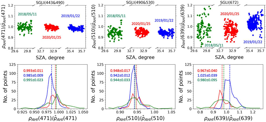
FIGURE 5. (Top) cross-calibration coefficients versus solar zenith angle, SZA, and (bottom) histograms of cross-calibration coefficients for AHI/SGLI at 471, 510, and 639 nm. The equivalent AHI reflectance ${\widehat{\rho }}_{AHI}$ at 471, 510, and 569 nm was generated using SGLI at 443 and 490 nm, 490 and 530 nm, and 672 nm, respectively. Different colors represent different dates. Vertical lines indicate the means, whose values, together with standard deviations, are specified in the insets.

FIGURE 6

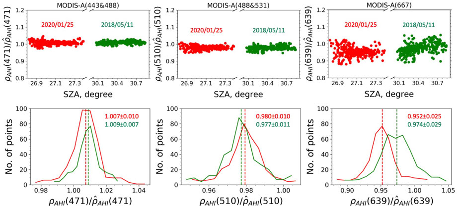
FIGURE 6. Same as Figure 5, but for the equivalent AHI reflectance ${\widehat{\rho }}_{AHI}$ at 471, 510, and 569 nm generated using MODIS-A 443&488 nm, 488&531 nm, and 667 nm.

FIGURE 7

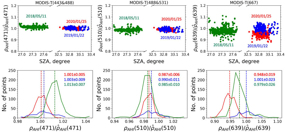
FIGURE 7. Same as Figure 5, but for the equivalent AHI reflectance ${\widehat{\rho }}_{AHI}$ at 471, 510, and 569 nm generated using MODIS-T 443&488 nm, 488&531 nm, and 667 nm.

The results of cross-calibration coefficients (mean and standard deviation) for pairs of geostationary and polar-orbiting sensors on different days are summarized in Tables 5, 6, 7. In comparison with AHI/MODIS-A and AHI/MODIS-T, for which the cross-calibration coefficients are very close to 1, i.e., generally less than 1% and about 2% difference from 1 for 471 nm and 510 nm, the AHI/SGLI ratios deviate from 1 by about 1% and 5%. The cross-calibration coefficients at 639 nm range from ∼0.94 to ∼1.02 for AHI/MODIS-A and AHI/MODIS-T, depending on the wavelength used for spectral matching and day of observation, and show about 3% deviation from 1 for AHI/SGLI. In general, the standard deviations are less than 0.02 at 471 and 510 nm but increase more than twofold at 639 nm for each sensor pair. In addition, the standard deviations of cross-calibration coefficients for AHI/MODIS-A and AHI/MODIS-T at 639 nm both increase as the wavelength used to generate equivalent AHI data increases, i.e., from 645 nm to 667 nm and 678 nm, which is expected as the spectral matching accuracy decreases when the center of the MODIS band is shifted from the AHI center wavelength of 639 nm (Table 2). The measurement errors on the average cross-calibration coefficients of the individual samples (days), can therefore be estimated as $SD/\sqrt{N}$ where $SD$ is the standard deviation and $N$ is the number of coincidences per day, which yields values of 0.0007–0.0027 for AHI/SGLI and 0.0002–0.0015 for AHI/MODIS-A and AHI/MODIS-T.

TABLE 5

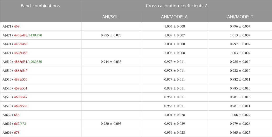
TABLE 5. The means and standard deviations of the cross-calibration coefficients A for AHI/SGLI, AHI/MODIS-A, and AHI/MODIS-T, obtained using MODIS (red fonts) and SGLI (green fonts) band combinations on 11 May 2018.

TABLE 6

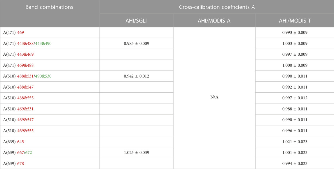
TABLE 6. Same as Table 5, but for coincidences obtained on 22 January 2019.

TABLE 7

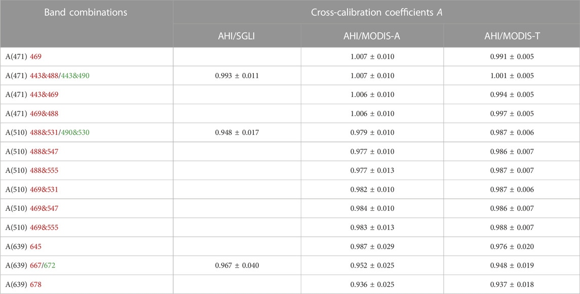
TABLE 7. Same as Table 6, but for coincidences obtained on 25 January 2020.

5.2.2 Pairs of polar-orbiting sensors

After the cross-calibration coefficients for the sensor pairs AHI/SGLI, AHI/MODIS-A, and AHI/MODIS-T are determined, it is straightforward to calculate the cross-calibration coefficients of the polar-orbiting sensors. Assume that the cross-calibration coefficients of sensors A/B and A/C at band $i$ are expressed as $R_{i\left(AB\right)}\pm {\delta }_{i\left(AB\right)}$ and $R_{i\left(AC\right)}\pm {\delta }_{i\left(AC\right)}$, as indicated in Section 5.2.1, the cross-calibration coefficient for C/B is then calculated as $R_{i\left(CB\right)}=R_{i\left(AB\right)}/R_{i\left(AC\right)}$, and the associated uncertainty as ${\delta }_{i\left(CB\right)}=R_{i\left(AB\right)}/R_{i\left(AC\right)}\sqrt{{\left({\delta }_{i\left(AB\right)}/R_{i\left(AB\right)}\right)}^2+{\left({\delta }_{i\left(AC\right)}/R_{i\left(AC\right)}\right)}^2}$ since the fractional errors add in quadrature. This results in two cross-calibration coefficients for MODIS-A/MODIS-T (11 May 2018 and 25 January 2020), three two for SGLI/MODIS-T (11 Ma y 2018, 22 January 2019 and 25 January 2020), and two for SGLI/MODIS-A (11 May 2018, 25 January 2020). The uncertainty δ_i(CB) comes mainly from three different sources, in addition to instrument noise: 1) spectral band matching, 2) processing of satellite images into level-1b, and 3) correction of gaseous absorption. Furthermore, the AHI imagery was remapped to the SGLI/MODIS latitude-longitude grid, which introduces uncertainties. The errors from these various sources interact; how they propagate to yield the final cross-calibration uncertainty is complicated and difficult to untangle and hence not discussed here. It is assumed, however, that they constitute a Gaussian noise with zero mean. Note that δ_i(CB) does not include uncertainties in the calibration coefficients of individual sensors, which may bias the sample averages. In other words, the averages and measurement errors obtained for each day (i.e., each sample) correspond to one realization of the cross-calibration coefficients, since it is assumed that these coefficients do not change during the period of that day’s measurements.

The following procedure describes how to get an estimate of the cross-calibration coefficients and their uncertainties using values from different days. Given that the cross-calibration coefficients of band $i$ are from a distribution with mean ${\mu }_i$ and variance ${{\sigma }_i}^2$ and independent measurements are made at each day $j$ with known error (i.e., $R_{i,j}\pm {\delta }_{i,j}$), the inverse-variance weighted average which minimizes the variance of the weighted average is used to represent ${\mu }_i$ (Hartung et al., 2008):

${\mu }_i={\displaystyle \sum }_{j=1}^n{\omega }_{i,j}{R}_{i,j}(7)$

with the weights ${\omega }_{i,j}$ expressed as:

${\omega }_{i,j}=\frac{1/\left({{\sigma }_i}^2+{{\delta }_{i,j}}^2\right)}{{\sum }_{j=1}^{n}1/\left({{\sigma }_i}^2+{{\delta }_{i,j}}^2\right)}(8)$

and the uncertainty of ${\mu }_i$ calculated as:

${{\delta }_{\mu }}_i=\sqrt{\frac{1}{{\sum }_{j=1}^{n}1/\left({{\sigma }_i}^2+{{\delta }_{i,j}}^2\right)}}(9)$

where $n$ is the total number of days. If the variances of the measurements ${\delta }_{i,j}$ are all equal, the inverse-variance weighted average becomes the simple average. Since the population standard deviation ${\sigma }_i$ is unknown, estimating ${\sigma }_i$ and the weights ${\omega }_{i,j}$ can be done iteratively.

The detailed iterative procedure is described as below. Given the estimate ${\widehat{\sigma }}_{i;k}$ of ${\sigma }_i$ obtained after $k$ iterations, the weights are updated as

${\omega }_{i,j;k}=\frac{1/\left({{\widehat{\sigma }}_{i;k}}^2+{{\delta }_{i,j}}^2\right)}{{\sum }_{j=1}^{n}1/\left({{\widehat{\sigma }}_{i;k}}^2+{{\delta }_{i,j}}^2\right)}(10)$

with the updated estimated (weighted) mean as

${\mu }_{i;k}={\displaystyle \sum }_{j=1}^n{\omega }_{i,j;k}{R}_{i,j}(11)$

Then the estimate of ${\widehat{\sigma }}_{i;k+1}$ in the next iteration can be updated as

${\widehat{\sigma }}_{i;k+1}=\sqrt{\frac{n}{n-1}{\displaystyle \sum }_{j=1}^n{\omega }_{i,j;k}{\left(R_{i,j}-{\mu }_{i;k}\right)}^2-\frac{1}{n}{\displaystyle \sum }_{j=1}^n{{\delta }_{i,j}}^2}(12)$

Specifically, $\frac{n}{n-1}{\displaystyle \sum }_{j=1}^n{\omega }_{i,j;k}{\left(R_{i,j}-{\mu }_{i;k}\right)}^2$ is the total weighted standard deviation and $1/n{\displaystyle \sum }_{j=1}^n{{\delta }_{i,j}}^2$ is the averaged measurement error. Iterations are performed until ${\widehat{\sigma }}_i$ converges. The initial estimate ${\widehat{\sigma }}_{i;0}$ is set to be the unweighted standard deviation calculated using $R_{i,j}$. The final estimates of ${\mu }_i$, ${\sigma }_i$, and ${{\delta }_{\mu }}_i$ are regarded as the expected cross-calibration coefficient, the standard deviation of the population, and the associated uncertainty.

In the present study, however, as already mentioned in Section 5.2.1, since we only have 3 days or even 2 days of data for some sensor pairs, it is difficult to estimate ${\sigma }_i$ correctly using the above procedure. This procedure should be used preferentially, however, when the number of samples (days) is sufficiently large. To overcome the lack of days, ${\sigma }_i$ is estimated from reported uncertainties on vicarious gains of the polar-orbiting sensors to cross-calibrate. The uncertainty on the AHI calibration coefficients is not needed because they can be assumed constant when cross-calibrating AHI and each of the polar-orbiting sensors during the same day, i.e., their effect disappears when forming $R_{i\left(CB\right)}=R_{i\left(AB\right)}/R_{i\left(AC\right)}$. In Table 2 of Franz et al. (2007), the standard deviations of SeaWiFS vicarious gains are listed, and they are representative of what is achieved for MODIS-A and -T. Based on this, the uncertainties on the MODIS-A and MODIS-T TOA calibration coefficients after SVC are approximated as 0.009, 0.009, 0.008, 0.008, 0.008, 0.008, 0.007, 0.007, and 0.007 for 443 nm, 469 nm, 488 nm, 531 nm, 547 nm, 645 nm, 667 nm, and 678 nm, respectively. The uncertainties of the corresponding equivalent AHI reflectance at 471 nm, 510 nm, and 639 nm, i.e., ${∆}_i$ for equivalent AHI band $i$, expressed as linear combinations of MODIS bands (Table 2), can then be estimated as $\sqrt{{\left(a{∆}_m\right)}^2+{\left(b{∆}_n\right)}^2}$ where $a$ and $b$ are the linear coefficients, and ${∆}_m$ and ${∆}_n$ represent the standard deviations of MODIS calibration coefficients at bands $m$ and $n$. Lastly, since the ratios of MODIS-A/MODIS-T TOA reflectance are close to 1, ${\sigma }_i$ can be estimated as $\sqrt{{∆}_{MODIS-A,i}{}^2+{∆}_{MODIS-T,i}{}^2}$, where ${∆}_{MODIS-A,i}$ and ${∆}_{MODIS-T,i}$ are the uncertainties using MODIS-A and MODIS-T band combinations. The uncertainties of SGLI/MODIS-A and SGLI/MODIS-T cross-calibration coefficients, therefore the standard deviation of the population, are estimated in a similar way, except that the standard deviations of SGLI cross-calibration coefficients are from Murakami et al. (2002).

The resulting cross-calibration coefficients for polar-orbiting sensor pairs are displayed in Table 8. The cross-calibration coefficients estimated on different days are within the uncertainty limits of the final estimates, confirming that the proposed procedure is valid, even with limited samples. It is revealed that MODIS-A and MODIS-T are well cross-calibrated, i.e., that the level 1b radiance of the two sensors is very close in the equivalent AHI bands, with differences of about 1% from unity for all band combinations and that those differences are generally within the uncertainties, except in a couple of cases where they are slightly larger. Note that even if MODIS-A and MODIS-T are well inter-calibrated with respect to the AHI bands of reference, given that the spectral bands of the two sensors are not the same, although very similar, we expect that the cross-calibration coefficients of two corresponding bands should slightly deviate from unity (the two instruments are not measuring the same radiance). When using band combinations mapped to a band of reference, it is possible that calibration uncertainties in different bands compensate. However, for our case, the cross-calibrations using various band combinations all yield good results, i.e., small cross-calibration differences from unity within uncertainties, strongly suggesting that the corresponding MODIS-A and MODIS-T bands used in the combinations are also well inter-calibrated.

TABLE 8

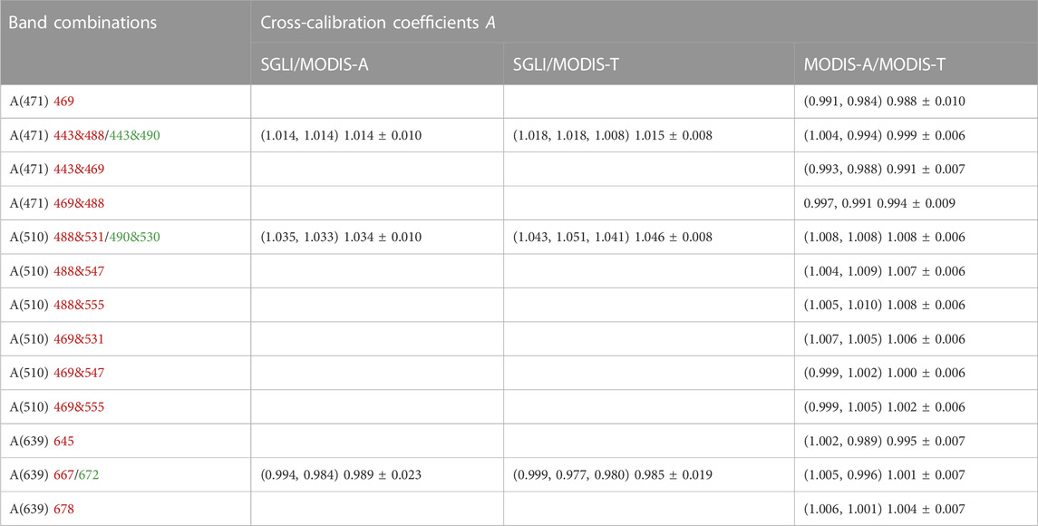
TABLE 8. The best estimate of cross-calibration coefficients A and associated uncertainties for SGLI/MODIS-A, SGLI/MODIS-T, and MODIS-A/MODIS-T, obtained using MODIS (red fonts) and SGLI (green fonts) band combinations. The cross-calibration coefficients obtained for individual days are listed in parentheses. See the main text for more details on how to get the best estimates.

In comparison, differences of 1.4%, 3.4%, and 1.1% with uncertainties of about 1.0%, 1.0%, and 2.3% are obtained between SGLI and MODIS-A calibration coefficients for equivalent AHI 443, 490, and 639 nm bands. Similar results are obtained between SGLI and MODIS-T, with the differences of 1.5%, 4.6%, and 1.5% and uncertainties of 0.8%, 0.8%, and 1.9%, respectively. The uncertainties of SGLI/MODIS-A cross-calibration coefficients are larger than those of SGLI/MODIS-T because only 2 days of data are available for SGLI/MODIS-A but 3 days for SGLI/MODIS-T, confirming that adding more days of observations will reduce the uncertainties. The large uncertainties at 639 nm are mainly caused by the relatively large standard deviation of SGLI TOA reflectance at 672 nm and the spectral matching which is due to AHI not having a similar red band as SGLI and MODIS-A/MODIS-T. As the cross-calibration coefficients differ significantly from unity within the estimated uncertainties at AHI 510 nm, it is concluded that differences do exist between SGLI and MODIS-A and between SGLI and MODIS-T TOA signals for at least one of the blue-green wavelengths (443, 490, and 530 nm), if not all of them, but the method does not allow one to specify which ones. Note that the uncertainties are mostly due to the population standard deviation ${\sigma }_i$, because the number of observations is numerous for the selected days. This may not be the case for days with less observations, i.e., the influence of the standard deviation of each sample (observations during a given day) becomes more important.

In a typical open-ocean scenario of oligotrophic waters, where the absorption of blue light is minimal, water-leaving signals contribute ∼10% of the total signal at the TOA in the blue-green spectral range (Gordon, 1997). As such, the about 4% difference in the SGLI/MODIS-A and SGLI/MODIS-T calibration for the band combination using 490 and 510 nm would result in a much larger difference on the water-leaving signal than the acceptable uncertainty for ocean color applications, i.e., 5% (IOCCG, 2013), if the same atmospheric correction scheme were applied to SGLI and MODIS data. It is quite possible that such differences may introduce significant discrepancies between the downstream ocean-color products by SGLI and MODIS-A and -T. As indicated in Murakami et al. (2022), however, the atmospheric correction scheme applied to SGLI is different from that used for MODIS-A and MODIS-T, which may eventually compensate for the differences in TOA signals. In addition, SVC of SGLI was performed using the in situ measurements from both MOBY and BOUSSOLE, as compared to the OBPG vicarious calibration that only utilized MOBY measurements. In Table 2 of their paper, Murakami et al. (2022) reported differences of vicarious calibration gains depending on the in situ datasets and aerosol LUTs used. About 1% difference in the gains were found for SGLI at 443, 490, and 530 nm while the gains at 672 nm were almost identical when using LUT-A and MOBY + BOUSSOLE, i.e., the method applied to SGLI, versus using LUT-B and MOBY, i.e., the method applied to MODIS-A and -T. Consequently, the different atmospheric correction and SVC applied to SGLI and MODIS-A and -T may reduce the impact of TOA signal discrepancy on the derived ocean-color products. This requires further investigation, for example by directly comparing the ocean color products from the three instruments. The results emphasize that applying a unique atmospheric correction scheme for all sensors, which may be desirable to generate consistent time series, requires performing the SVC in the same way, using the same atmospheric correction scheme.

6 Summary and conclusion

This study provides a generic methodology to cross-calibrate satellite ocean-color sensors in polar orbit. The methodology utilizes a geostationary sensor of reference, i.e., in our case AHI on board Himawari-8, which acts as the intermediary between the ocean-color sensors considered, namely SGLI, MODIS-A, and MODIS-T. This allows one to find numerous coincident measurements in space, time, and geometry over oceanic regions, an advantage over other cross-calibration techniques. The procedure consists of cross-calibrating each of the polar orbiting ocean-color sensors against the referenced geostationary sensor separately and then ratioing the cross-calibration coefficients.

Spectral matching of AHI spectral bands was first performed using a single band or two band combinations of SGLI, MODIS-A, and MODIS-T, based on radiative transfer simulations for various of geometry and geophysical conditions. Results show that the TOA reflectance at AHI blue and green wavelengths can be accurately reconstructed with RMS differences less than 1%. The spectral matching accuracy is degraded for AHI 639 nm, with RMS differences above 3% when using SGLI at 672 nm and MODIS-A and -T at 678 nm. This is because the SGLI and MODIS red bands are quite different from the AHI band at 639 nm, i.e., with narrower bandwidths and different band centers. Although the AHI reflectance at wavelengths longer than 639 nm, i.e., 857 and 1,610 nm, can be precisely reconstructed, large radiometric noise from the AHI imagery makes it more difficult to cross-calibrate polar-orbiting ocean sensors with sufficient accuracy at those wavelengths. Such large noise is expected since AHI is not designed for ocean targets but for meteorological research. Therefore, and also because of the small number of days to determine the unknown population variance of the polar-orbiting sensors’ calibration coefficients in the NIR and SWIR, only AHI data at 471, 530, and 639 nm was used to estimate cross-calibration coefficients, and these bands were the bands of reference.

Application of the methodology to MODIS-A, MODIS-T, and SGLI using AHI quantified the magnitude of inter-calibration coefficients in comparable spectral bands or combination of spectral bands. Only 3 days with mostly clear sky ocean pixels were selected, i.e., 11 May 2018, 22 January 2019, and 25 January 2020. Numerous coincident pixels were obtained from images acquired on the three different dates and used to determine the cross-calibration coefficients and associated uncertainties. It was found that MODIS-A and MODIS-T after SVC are well cross-calibrated in the bands of reference, with differences of about 1% from unity, generally within the uncertainties, for all band combinations. Using diverse band combinations further suggested that the MODIS-A and MODIS-T individual bands at 443, 469, 488, 531, 547, and 555 nm are also well cross-calibrated. In comparison, larger differences, i.e., 1.4%, 3.4%, and 1.1%, between SGLI and MODIS-A were found for the equivalent AHI bands at 471, 510, and 639 nm. Similar results were obtained between SGLI and MODIS-T, with differences of 1.5%, 4.6%, and 1.5%, respectively. The uncertainty of the cross-calibration coefficients between SGLI and MODIS was ±0.8%–1.0% at 471 and 510 nm, and larger, i.e., ±1.9%–2.3% at 639 nm. This larger uncertainty at 639 nm can be attributed to the relatively large uncertainty in SGLI TOA signals at 672 nm as well as the spectral matching error and AHI radiometric noise which result in larger measurement errors at this wavelength. The results also suggest that the uncertainties of cross-calibration coefficients can be reduced when adding more days of observations. These cross-calibration differences are above the estimated uncertainties at 510 nm, affirming that significant differences exist between SGLI and MODIS-A and -T TOA signals, especially in the blue-green spectral range. The differences of about 4% in the blue and green between SGLI and MODIS signals far exceed the absolute radiometric calibration uncertainty required for ocean color remote sensing (i.e., a fraction of 1%) and may introduce discrepancies between ocean-color products generated from SGLI and MODIS-A and -T imagery if the same atmospheric correction scheme were applied. However, the different atmospheric correction and SVC procedures applied to SGLI and MODIS may alleviate the impact of TOA signal discrepancies between SGLI and MODIS-A and MODIS-T on downstream ocean color products.

The findings provide the basis for a normalized calibration of SGLI, MODIS-A, and MODIS-T, which is important to generating consistent long-term ocean-color products from multiple satellites. Basically, we expect the radiance measured at a certain wavelength by all the sensors in given geophysical and geometric conditions to be the same. However, as mentioned above, this might not be the case when using level 1b data after SVC adjustment if the atmospheric correction scheme and SVC procedure are not the same for all sensors, i.e., caution must be exercised in the interpretation of deviations from unity of the cross-calibration coefficients. The method proposed in this study can be applied operationally, and to other optical sensors operating in polar orbit. It can also be performed prior to SVC, as this calibration may be considered as part of the atmospheric correction process. Due to the limitation of the AHI spectral bands, the cross-calibration using this intermediary sensor was mostly accomplished using multiple bands instead of a single band. The relatively high AHI radiometric noise, the limited number of days, and the large uncertainty of the polar-orbiting sensors’ calibration coefficients (or the lack of information about their uncertainty) in the NIR and SWIR prevented cross-calibrating in this spectral range. Yet the methodology is generally applicable to those longer wavelengths, provided that the number of coincidences during a day and the number of days are sufficiently numerous, the spectral matching is accurate, and the population variance of the calibration coefficients is not too large; otherwise, the resulting cross-calibration coefficients might be too inaccurate for meaningful conclusions. The methodology, however, has great potential with geostationary sensors that have ocean color capabilities. The Geostationary Ocean Color Imager (GOCI) follow-on, GOCI-II (Ahn and Park, 2020), in particular, collects data in 12 narrow ultraviolet, visible, and near-infrared bands at 0.25 km resolution, allowing direct band-to-band mapping with polar-orbiting ocean color sensors. This was not possible with GOCI, which only observed in local area mode around South Korea (Choi et al., 2012; Ryu et al., 2012). But such geostationary sensors, which have low radiometric noise and narrow spectral bands, require more time to acquire a scene than sensors onboard weather geostationary satellites, yielding less frequent coincident observations. In fact, GOCI-II observes 10 times during daytime in regional mode, but only once a day in full disk mode, making it difficult to obtain proper coincidences in low-latitude regions for cross-calibrating polar-orbiting sensors. Nevertheless, other geostationary sensors such as the Spinning Enhanced Visible InfraRed Imager on board Meteosat Second Generation, the Advanced Baseline Imager carried by the Geostationary Operational Environmental Studies R series, and the Flexible Combined Imager onboard Meteosat Third Generation, though with restricted number of spectral bands and not primarily intended for ocean research, can still serve as useful references in the cross-calibration of ocean-color sensors in polar orbit.

Data availability statement

Publicly available datasets were analyzed in this study. This data can be found here: JAXA’s P-Tree system (https://www.eorc.jaxa.jp/ptree/index.html), NASA OBPG (https://oceancolor.gsfc.nasa.gov), JAXA’s G-Portal (https://gportal.jaxa.jp/gpr/).

Author contributions

Conceptualization, methodology and investigation, JT and RF; writing—original draft preparation, JT; writing—review and editing, RF and HM; supervision, RF. All authors have read and agreed to the published version of the manuscript.

Funding

This work was funded by JAXA under Contract 22RT000268 and NASA under Grant 80NSSC21K1661.

Acknowledgments

The authors gratefully acknowledge the NASA OBPG and JAXA EORC for generating, maintaining, and distributing the Level-1 satellite products used in the study. They thank Dr. Pierre-Yves Deschamps (retired), University of Lille, for helpful discussions. The reviewers’ comments were also greatly appreciated.

Conflict of interest

The authors declare that the research was conducted in the absence of any commercial or financial relationships that could be construed as a potential conflict of interest.

Publisher’s note

All claims expressed in this article are solely those of the authors and do not necessarily represent those of their affiliated organizations, or those of the publisher, the editors and the reviewers. Any product that may be evaluated in this article, or claim that may be made by its manufacturer, is not guaranteed or endorsed by the publisher.

References

Ahn, J.-H., and Park, Y.-J. (2020). Estimating water reflectance at near-infrared wavelengths for turbid water atmospheric correction: A preliminary study for GOCI-II. Remote Sens. 12, 3791. doi:10.3390/rs12223791

CrossRef Full Text | Google Scholar

Ahn, J.-H., Park, Y.-J., Kim, W., Lee, B., and Oh, I. S. (2015). Vicarious calibration of the geostationary Ocean Color imager. Opt. Express 23, 23236–23258. doi:10.1364/OE.23.023236

PubMed Abstract | CrossRef Full Text | Google Scholar

Antoine, D., Chami, M., Claustre, H., d’Ortenzio, F., Morel, A., Becu, G., et al. (2006). Boussole: A joint CNRS-INSU, esa, cnes, and NASA ocean color calibration and validation activity. Greenbelt, MD, USA: NASA.NASA/TM-2006-214147

Google Scholar

Antoine, D., d’Ortenzio, F., Hooker, S. B., Bécu, G., Gentili, B., Tailliez, D., et al. (2008). Assessment of uncertainty in the ocean reflectance determined by three satellite ocean color sensors (MERIS, SeaWiFS and MODIS-A) at an offshore site in the Mediterranean Sea (BOUSSOLE project). J. Geophys. Res. Oceans 113, C07013. doi:10.1029/2007JC004472

CrossRef Full Text | Google Scholar

Atkinson, P., Sargent, I., Foody, G., and Williams, J. (2007). Exploring the geostatistical method for estimating the Signal-to-Noise ratio of images. Photogrammetric Eng. Remote Sens. 73, 841–850. doi:10.14358/PERS.73.7.841

CrossRef Full Text | Google Scholar

Barnes, B. B., Hu, C., Bailey, S. W., Pahlevan, N., and Franz, B. A. (2021). Cross-calibration of MODIS and VIIRS long near infrared bands for ocean color science and applications. Remote Sens. Environ. 260, 112439. doi:10.1016/j.rse.2021.112439

CrossRef Full Text | Google Scholar

Bisson, K. M., Boss, E., Werdell, P. J., Ibrahim, A., Frouin, R., and Behrenfeld, M. J. (2021). Seasonal bias in global ocean color observations. Appl. Opt. 60, 6978–6988. doi:10.1364/AO.426137

PubMed Abstract | CrossRef Full Text | Google Scholar

Cao, C., Weinreb, M. P., and Xu, H. (2004). Predicting simultaneous nadir overpasses among polar-orbiting meteorological satellites for the intersatellite calibration of radiometers. J. Atmos. Ocean. Technol. 21, 537–542. doi:10.1175/1520-0426(2004)021<0537:psnoap>2.0.co;2

CrossRef Full Text | Google Scholar

Chang, T., Xiong, X., and Angal, A. (2019). Terra and Aqua MODIS TEB intercomparison using Himawari-8/AHI as reference. J. Appl. Remote Sens. 13, 017501. 10.1117/1.JRS.13. 017501.

CrossRef Full Text | Google Scholar

Chen, S., Zheng, X., Li, X., Wei, W., Du, S., and Guo, F. (2021). Vicarious radiometric calibration of ocean color bands for FY-3D/MERSI-II at lake qinghai, China. Sensors 21, 139. doi:10.3390/s21010139

CrossRef Full Text | Google Scholar

Chiles, J., and Delfiner, P. (1999). Geostatistics: Modeling spatial uncertainty. New York, NY, USA: Wiley, 69.

Google Scholar

Choi, J.-K., Park, Y. J., Ahn, J. H., Lim, H.-S., Eom, J., and Ryu, J.-H. (2012). GOCI, the world’s first geostationary ocean color observation satellite, for the monitoring of temporal variability in coastal water turbidity. J. Geophys. Res. Oceans 117. doi:10.1029/2012JC008046

CrossRef Full Text | Google Scholar

Clark, D. K., Gordon, H. R., Voss, K. J., Ge, Y., Broenkow, W., and Trees, C. (1997). Validation of atmospheric correction over the oceans. J. Geophys. Res. Atmos. 102, 17209–17217. doi:10.1029/96JD03345

CrossRef Full Text | Google Scholar

Cressie, N. (1993). Statistics for spatial data. New York, NY, USA: Wiley, 928.

Google Scholar

Datla, R., Rice, J., Lykke, K., Johnson, B., Butler, J., and Xiong, X. (2011). Best practice guidelines for pre-launch characterization and calibration of instruments for passive optical remote sensing. J. Res. Natl. Inst. Stand. Technol. 116, 621–646. doi:10.6028/jres.116.009

PubMed Abstract | CrossRef Full Text | Google Scholar

Delwart, S., and Bourg, L. (2011). “Radiometric calibration of MERIS,” in Sensors, systems, and next- generation satellites XV. Editors R. Meynart, S. P. Neeck, and H. Shimoda (Bellingham, Washington DC, USA: International Society for Optics and Photonics SPIE), 8176, 817613. doi:10.1117/12.895090

CrossRef Full Text | Google Scholar

Djavidnia, S., Me ́lin, F., and Hoepffner, N. (2010). Comparison of global ocean colour data records. Ocean Sci. 6, 61–76. doi:10.5194/os-6-61-2010

CrossRef Full Text | Google Scholar

Eplee, R. E., Sun, J.-Q., Meister, G., Patt, F. S., Xiong, X., and McClain, C. R. (2011). Cross calibration of SeaWiFS and MODIS using on-orbit observations of the moon. Appl. Opt. 50, 120–133. doi:10.1364/AO.50.000120

PubMed Abstract | CrossRef Full Text | Google Scholar

Fougnie, B., Deschamps, P.-Y., and Frouin, R. (1999). Vicarious calibration of the POLDER ocean color spectral bands using in situ measurements. IEEE Trans. Geoscience Remote Sens. 37, 1567–1574. doi:10.1109/36.763267

CrossRef Full Text | Google Scholar

Fougnie, B., Bracco, G., Lafrance, B., Ruffel, C., Hagolle, O., and Tinel, C. (2007). PARASOL inflight calibration and performance. Appl. Opt. 46, 5435–5451. doi:10.1364/AO.46.005435

PubMed Abstract | CrossRef Full Text | Google Scholar

Franz, B. A., Bailey, S. W., Werdell, P. J., and McClain, C. R. (2007). Sensor-independent approach to the vicarious calibration of satellite ocean color radiometry. Appl. Opt. 46, 5068–5082. 10.1364/AO.46.005068.

PubMed Abstract | CrossRef Full Text | Google Scholar

Frouin, R. J., Franz, B. A., Ibrahim, A., Knobelspiesse, K., Ahmad, Z., Cairns, B., et al. (2019). Atmospheric correction of satellite ocean-color imagery during the PACE era. Front. Earth Sci. 7. doi:10.3389/feart.2019.00145

PubMed Abstract | CrossRef Full Text | Google Scholar

Gelaro, R., McCarty, W., Sua ́rez, M. J., Todling, R., Molod, A., Takacs, L., et al. (2017). The modern-era retrospective analysis for research and applications, version 2 (MERRA-2). J. Clim. 30, 5419–5454. doi:10.1175/JCLI-D-16-0758.1

CrossRef Full Text | Google Scholar

Glover, D. M., Doney, S. C., Oestreich, W. K., and Tullo, A. W. (2018). Geostatistical analysis of mesoscale spatial variability and error in SeaWiFS and MODIS/Aqua global ocean color data. J. Geophys. Res. Oceans 123, 22–39. doi:10.1002/2017JC013023

CrossRef Full Text | Google Scholar

Gordon, H. R. (1997). Atmospheric correction of ocean color imagery in the Earth observing system era. J. Geophys. Res. Atmos. 102, 17081–17106. 10.1029/96JD02443.

CrossRef Full Text | Google Scholar

Hagolle, O., Goloub, P., Deschamps, P.-Y., Cosnefroy, H., Briottet, X., Bailleul, T., et al. (1999). Results of POLDER in-flight calibration. IEEE Trans. Geoscience Remote Sens. 37, 1550–1566. doi:10.1109/36.763266

CrossRef Full Text | Google Scholar

Hartung, J., Knapp, G., and Sinha, B. K. (2008). Statistical meta-analysis with applications. New York, NY, USA: Wiley, 272.

Google Scholar

Hlaing, S., Gilerson, A., Foster, R., Wang, M., Arnone, R., and Ahmed, S. (2014). Radiometric calibration of ocean color satellite sensors using AERONET-OC data. Opt. Express 22, 23385–23401. doi:10.1364/OE.22.023385

PubMed Abstract | CrossRef Full Text | Google Scholar

IOCCG, (2013). In-flight calibration of satellite ocean-Colour sensors. Dartmouth, Canada: IOCCG International Ocean-Colour Coordinating Group.

Google Scholar

JMA, (2017). Improvement of Himawari-8 observation data quality. Kiyose, Tokyo, Japan: Meteorological Satellite Center Japan Meteorological Agency. Available online: https://www.data.jma.go.jp/mscweb/en/oper/eventlog/Improvement_of_Himawari-8_data_quality.pdf.

Google Scholar

Kang, G., Coste, P., Youn, H., Faure, F., and Choi, S. (2010). An in-orbit radiometric calibration method of the geostationary ocean color imager. IEEE Trans. Geoscience Remote Sens. 48, 4322–4328. doi:10.1109/TGRS.2010.2050329

CrossRef Full Text | Google Scholar

Kotchenova, S. Y., Vermote, E. F., Matarrese, R., Frank, J., and Klemm, J. (2006). Validation of a vector version of the 6S radiative transfer code for atmospheric correction of satellite data. Part I: Path radiance. Appl. Opt. 45, 6762–6774. doi:10.1364/AO.45.006762

PubMed Abstract | CrossRef Full Text | Google Scholar

Kotchenova, S. Y., and Vermote, E. F. (2007). Validation of a vector version of the 6S radiative transfer code for atmospheric correction of satellite data. Part II. homogeneous lambertian and anisotropic surfaces. Appl. Opt. 46, 4455–4464. doi:10.1364/AO.46.004455

PubMed Abstract | CrossRef Full Text | Google Scholar

Kwiatkowska, E. J., Franz, B. A., Meister, G., McClain, C. R., and Xiong, X. (2008). Cross calibration of ocean-color bands from moderate resolution imaging spectroradiometer on Terra platform. Appl. Opt. 47, 6796–6810. doi:10.1364/AO.47.006796

PubMed Abstract | CrossRef Full Text | Google Scholar

Lacherade, S., Fougnie, B., Henry, P., and Gamet, P. (2013). Cross calibration over desert sites: Description, methodology, and operational implementation. IEEE Trans. Geoscience Remote Sens. 51, 1098–1113. doi:10.1109/TGRS.2012.2227061

CrossRef Full Text | Google Scholar

Martiny, N., Santer, R., and Smolskaia, I. (2005). Vicarious calibration of meris over dark waters in the near infrared. Remote Sens. Environ. 94, 475–490. doi:10.1016/j.rse.2004.11.008

CrossRef Full Text | Google Scholar

Meister, G., and Franz, B. A. (2011). “Adjustments to the MODIS Terra radiometric calibration and polarization sensitivity in the 2010 reprocessing,” in Earth observing systems XVI. Editors J. J. Butler, X. Xiong, and X. Gu (Bellingham, Washington DC, USA: International Society for Optics and Photonics SPIE), 8153, 815308. doi:10.1117/12.891787

CrossRef Full Text | Google Scholar

Mélin, F. (2010). Global distribution of the random uncertainty associated with satellite-derived Chl a. IEEE Geoscience Remote Sens. Lett. 7, 220–224. doi:10.1109/LGRS.2009.2031825

CrossRef Full Text | Google Scholar

Mélin, F., Sclep, G., Jackson, T., and Sathyendranath, S. (2016). Uncertainty estimates of remote sensing reflectance derived from comparison of ocean color satellite data sets. Remote Sens. Environ. 177, 107–124. doi:10.1016/j.rse.2016.02.014

CrossRef Full Text | Google Scholar

Morel, A., and Maritorena, S. (2001). Bio-optical properties of oceanic waters: A reappraisal. J. Geophys. Res. Oceans 106, 7163–7180. doi:10.1029/2000JC000319

CrossRef Full Text | Google Scholar

Murakami, H., Antoine, D., Vellucci, V., and Frouin, R. (2022). System vicarious calibration of GCOM- C/SGLI visible and near-infrared channels. J. Oceanogr. 78, 245–261. 10.1007/s10872-022-00632-x.

CrossRef Full Text | Google Scholar

Murakami, H., Kachi, M., Maeda, T., Shiomi, K., Tadono, T., Kaneko, Y., et al. (2019). JAXA agency report, global space-based inter-calibration system (GSICS). Available online: http://gsics.atmos.umd.edu/pub/Development/AnnualMeeting2019/3c_Murakami_JAXAReport.pptx (accessed on August 22, 2022).

Google Scholar

Murakami, H., Yoshida, M., Tanaka, K., Fukushima, H., Toratani, M., Tanaka, A., et al. (2005). Vicarious calibration of ADEOS-2 GLI visible to shortwave infrared bands using global datasets. IEEE Trans. Geoscience Remote Sens. 43, 1571–1584. doi:10.1109/TGRS.2005.848425

CrossRef Full Text | Google Scholar

Okamura, Y., Hashiguch, T., Urabe, T., Tanaka, K., Yoshida, J., Sakashita, T., et al. “Pre-launch characterisation and in-orbit calibration of GCOM-C/SGLI,” in IGARSS 2018 - 2018 IEEE International Geoscience and Remote Sensing Symposium, Valencia, Spain, July, 2018, 6651–6654. 10.1109/IGARSS.2018.8519151 .

Google Scholar

Okuyama, A., Takahashi, M., Date, K., Hosaka, K., Murata, H., Tabata, T., et al. (2018). Validation of Himawari-8/Ahi radiometric calibration based on two years of in-orbit data. J. Meteorological Soc. Jpn. Ser. II 96B, 91–109. doi:10.2151/jmsj.2018-033

CrossRef Full Text | Google Scholar

Qin, Y., and McVicar, T. R. (2018). Spectral band unification and inter-calibration of Himawari AHI with MODIS and VIIRS: Constructing virtual dual-view remote sensors from geostationary and low-Earth-orbiting sensors. Remote Sens. Environ. 209, 540–550. doi:10.1016/j.rse.2018.02.063

CrossRef Full Text | Google Scholar

Ryu, J.-H., Han, H.-J., Cho, S., Park, Y.-J., and Ahn, Y.-H. (2012). Overview of geostationary Ocean Color imager (GOCI) and GOCI data processing system (GDPS). Ocean Sci. J. 47, 223–233. doi:10.1007/s12601-012-0024-4

CrossRef Full Text | Google Scholar

Sathyendranath, S., Brewin, R. J., Brockmann, C., Brotas, V., Calton, B., Chuprin, A., et al. (2019). An ocean-colour time series for use in climate studies: The experience of the Ocean-Colour Climate Change Initiative (OC-CCI). Sensors 19, 4285. doi:10.3390/s19194285

PubMed Abstract | CrossRef Full Text | Google Scholar

Sayer, A. M., Hsu, N. C., Bettenhausen, C., Holz, R. E., Lee, J., Quinn, G., et al. (2017). Cross-calibration of S-NPP VIIRS moderate-resolution reflective solar bands against MODIS Aqua over dark water scenes. Atmos. Meas. Tech. 10, 1425–1444. doi:10.5194/amt-10-1425-2017

PubMed Abstract | CrossRef Full Text | Google Scholar

Sun, J. -Q., Xiong, X., Barnes, W. L., and Guenther, B. (2007). MODIS reflective solar bands on-orbit lunar calibration. IEEE Trans. Geoscience Remote Sens. 45, 2383–2393. doi:10.1109/TGRS.2007.896541

CrossRef Full Text | Google Scholar

Tanaka, K., Okamura, Y., Mokuno, M., Amano, T., and Yoshida, J. (2018). “First year on-orbit calibration activities of SGLI on GCOM-C satellite,” in Earth observing missions and sensors: Development, implementation, and characterization. Editors X. Xiong, and T. Kimura (Bellingham, Washington DC, USA: International Society for Optics and Photonics SPIE), 10781, 107810Q. doi:10.1117/12.2324703V

CrossRef Full Text | Google Scholar

Urabe, T., Xiong, X., Hashiguchi, T., Ando, S., Okamura, Y., Tanaka, K., et al. “Lunar calibration inter-comparison of sgli, modis and viirs,” in IGARSS 2019 - 2019 IEEE International Geoscience and Remote Sensing Symposium, Yokohama, Japan, August, 2019, 8481–8484. 10.1109/IGARSS.2019.8897892 .

Google Scholar

Urabe, T., Xiong, X., Hashiguchi, T., Ando, S., Okamura, Y., and Tanaka, K. (2020). Radiometric model and inter-comparison results of the SGLI-VNR on-board calibration. Remote Sens. 12, 69. doi:10.3390/rs12010069

CrossRef Full Text | Google Scholar

Xiong, X., Angal, A., Chang, T., Chiang, K., Lei, N., Li, Y., et al. (2020). MODIS and VIIRS calibration and characterization in support of producing long-term high-quality data products. Remote Sens. 12, 3167. doi:10.3390/rs12193167

CrossRef Full Text | Google Scholar

Xiong, X., Angal, A., Twedt, K. A., Chen, H., Link, D., Geng, X., et al. (2019). MODIS reflective solar bands on-orbit calibration and performance. IEEE Trans. Geoscience Remote Sens. 57, 6355–6371. doi:10.1109/TGRS.2019.2905792

CrossRef Full Text | Google Scholar

Yu, F., and Wu, X. (2016). Radiometric inter-calibration between himawari-8 AHI and S-NPP VIIRS for the solar reflective bands. Remote Sens. 8, 165. doi:10.3390/rs8030165

CrossRef Full Text | Google Scholar

Zibordi, G., Mélin, F., and Berthon, J.-F. (2012). Intra-annual variations of biases in remote sensing primary ocean color products at a coastal site. Remote Sens. Environ. 124, 627–636. doi:10.1016/j.rse.2012.06.016

CrossRef Full Text | Google Scholar