 Mónica Retamosa Izaguirre*
 Jimy Barrantes Madrigal
- Universidad Nacional, Heredia, Costa Rica
Ecosystems are under a multitude of pressures, including land-use change, overexploitation, pollution, and climate change. Most studies, resources, and conservation efforts are allocated to protected areas, while anthropogenic activities in their surroundings may affect them in ways that are poorly understood. We evaluated soundscape structure in forests surrounded by protected or productive areas in central Costa Rica. We sampled soundscapes in 91 recording sites in Grecia Forest Reserve and Poas Volcano National Park, and surrounding areas with productive activities (predominantly agricultural and urban). We classified sampling sites into three clusters according to landscape entropy, forest amount, and fragmentation surrounding recording points: more fragmented, more conserved, and intermediate. The conserved cluster showed higher acoustic diversity or entropy, but lower acoustic complexity, shorter duration of sounds in all frequency ranges, and lower amount of energy in the biological frequency bands than the fragmented cluster. We additionally found a positive significant relationship between the amount of forest and acoustic entropy or diversity indices, but a negative relationship with acoustic activity or energy indices. Indices, such as spectral and temporal entropy, the entropy of spectral variance, and total entropy, seemed to be a better fit than acoustic complexity and bioacoustic indices as indicators of habitat conservation in this study. Acoustic indices revealed that the surrounding matrices of protected areas have an impact on acoustic environments. We encourage researchers and decision-makers to carefully interpret acoustic indices when evaluating habitats showing a higher value in acoustic energy or activity because this might not necessarily reflect either a high level of biodiversity or habitat conservation. Also, we highlight the importance of preserving undisturbed forested matrices around protected areas, as they are important for maintaining acoustic diversity.
1 Introduction
Ecosystems are under a multitude of pressures, including land use change, overexploitation, pollution, and climate change (Glaser 2015). As conservation measures, a series of protected areas have historically been established, which usually act as islands of protection in a matrix with different degrees of anthropogenic alteration. Most research, resources and conservation efforts are allocated to protected areas, while anthropogenic activities that take place in their surroundings, impact on them in ways that are poorly understood and managed.
Costa Rica has over 25% of its territory under some category of management within the system of conservation areas (Noches, 2005). These areas play an important role in the conservation of species and global processes (Pimm et al., 2018). But despite these initiatives and efforts to conserve forests, the change in land use and the overexploitation of its products as a result of population growth, still threaten their conservation (Maxwell et al., 2020). Some authors have suggested the need to assess complementary conservation strategies that also contribute to minimizing the problem of isolation of existing protected areas, such as the protection of wooded pastures, forest plantations, living fences, agroforestry systems, and even isolated fragments of natural or managed forest (Naoki et al., 2003).
The central conservation area (ACC), declared as a Biosphere Reserve, shelters 25 protected wild areas and has more than 250,000 ha of forests, which play a fundamental role in protecting biodiversity. In this area there is great biological diversity, the types of vegetation vary from tropical rain forest, low montane rain forest; to the subalpine pluvial or paramo of stunted vegetation in the Irazú Volcano. Currently, threats such as deforestation, hunting, the degradation of hydrographic basins, the expansion of agricultural frontiers and fragmentation due to urban expansion are present in the area. These activities generate significant pollution and exert strong pressure on protected wild areas (SINAC 2014). Other sources of pollution, such as noise, emerge with urbanization. Noise contributes to the degradation of ecosystems and affects wildlife, modifying the behavior and movement patterns of some species (Barber et al., 2011; Pijanowski et al., 2011).
Protected wilderness areas provide values associated with the appreciation of nature, both visual and acoustic, that can be exploited, as in the case of ecotourism, where the acoustic quality of the landscape is an essential element for visitors seeking sites free of noise (Farina et al., 2011). In tropical forests, high biodiversity contributes to a high diversity of natural sounds, so it is important to quantify the impact of the effects of human activity, in relation to sound, on wildlife (Pijanowski et al., 2011; Rodríguez et al., 2014). The loss of habitats and biodiversity causes the disappearance of natural sounds; that is why they must be managed as a natural resource that must be conserved (Pijanowski et al., 2011).
There is a constant need to consider the effect of anthropogenic activities on natural areas and surroundings as a possible source of ecosystem degradation and subsequent threat to biodiversity. It is important to conserve important sectors of land for protection, but at the same time manage the matrix surrounding the protected areas in order to minimize the negative impact of productive activities on them. For this, it is important to have effective monitoring mechanisms that can provide early warning of problems associated with ecosystem degradation in the surroundings of protected areas that could serve as a basis for decision-making and actions aimed at complying with environmental regulations in force in the country by the competent authorities and in agreement with the local stakeholders.
A variety of ecological methods and indicators have been used to assess the impacts of the anthropic activity on biodiversity and habitat conservation. However, one of the greatest challenges in conservation ecology and biology is the assessment of biodiversity through effective monitoring techniques, which allow covering wide spatial and temporal scales (Depraetere et al., 2012). This knowledge should be the basis for building more robust criteria that lead to better management of the territory, through a centralized monitoring system that allows researchers and decision-makers to have a good general perspective on the results obtained by monitoring programs on a national scale (Marsh and Trenham 2008). For example, cost-efficient techniques have been proposed to automatically collect large amounts of data at larger ecological and spatial scales, such as the recording of sounds to represent and quantify complete acoustic landscapes through a series of acoustic indices. These indices can be used for biodiversity assessments, research on community dynamics and landscape patterns (Sueur et al., 2014) since acoustic landscapes reflect the biophysical properties of the landscape, as well as the communication mechanisms between organisms, and they can function as an indicator of the state of biodiversity and ecosystems (Pijanowski et al., 2011).
Ecosystem sounds create an acoustic landscape composed of acoustic periodicities and frequencies emitted by biophysical entities of the ecosystem (Schafer 1977; Truax et al., 1984; Qi et al., 2008), which can be partitioned into anthropic (anthrophony), biological sources (biophony) and physical (geophony). The proportion between these different components of the acoustic landscape gives us an indication of the impact of the anthropic activity on ecosystems (Napoletano 2004; Qi et al., 2008; Joo et al., 2011; Pijanowski et al., 2011). In addition, there is another series of acoustic indices that estimate the level of complexity in terms of time, frequency, or amplitude of the sound (Sueur et al., 2014), which have been related to traditional biodiversity indices (Sueur et al., 2008; Farina et al., 2011; Depraetere et al., 2012; Gasc et al., 2013; Rodríguez et al., 2014; Pieretti et al., 2015; Trigg 2015; Machado et al., 2017; Mammides et al., 2017; Retamosa Izaguirre et al., 2018; Retamosa Izaguirre et al., 2021a; Retamosa Izaguirre et al. et al., 2021b).
We evaluated soundscape structure in forests surrounded by protected and productive (agricultural and urban) activities as an indicator of habitat conservation in central Costa Rica. In general, we expected that more conserved sites (landscapes with less entropy, larger size of forested patches, and less fragmented forest) would have a higher acoustic diversity and activity, as well as a higher proportion of biophonies than antrophonies. We discuss the use of acoustic indices as an early indicator of habitat conservation associated with productive activities in the surroundings of protected areas, as a tool to support decision-making and achieve conservation goals.
2 Methods
2.1 Study area
The Central Conservation Area (ACC) is located in the central region of the country, where it incorporates the entirety of the great metropolitan area (Silhouettes, 1987). Due to its location and urban development, it covers approximately 54% of the Costa Rican population in an area of 860 8000 ha, equivalent to 16.84% of the country’s area (SINAC 2014). Within its delimitation 31 protected areas are included in this conservation area.
The study was carried out in the northwestern region of the ACC, covering the protected areas of the Grecia Forest Reserve and the southern sector of the Poás Volcano National Park and its surroundings. The Grecia Forest Reserve is located approximately 14 km north of the city of Grecia and is bordered to the north by the Poás National Park (Leandro et al., 2016). It has an area of 2,000 ha with an elevation range between 1,600 and 2,500 m above sea level, which includes both areas of native vegetation and cypress and pine plantations (Maglianesi 2010). The average precipitation is 3600 mm per year, and it maintains an average temperature of 16 °C (Leandro et al., 2016). For its part, the Poás Volcano National Park is characterized by high rainfall with an annual rainfall that varies between 3,500 and 8,000 mm and a temperature that oscillates between 10 and 24 °C with an average of 14 °C (Boza 2001). Most of the protected area is covered by forests except places burned by volcanic eruptions, tourist areas and deforested areas. The canopy can generally reach up to 30 m in height, however it usually does not exceed 20 m. The understory is dense and most of the trees are covered with epiphytic plants such as mosses, bromeliads, orchids and ferns (González et al., 2019).
2.2 Landscape structure sampling
To sample the landscape structure around recording points, we overlaid a grid of 250 by 250 m over the study area and calculated 11 landscape metrics (Table 1) for those cells where recording sites were located. These landscape metrics were selected according to the effect reported in the literature on biodiversity (such as species richness, distribution, the abundance of populations, and genetic diversity, among others; Fahrig 2003), in addition to representing different aspects of interest to describe landscape conservation. We performed this analysis using ArcGIS (ESRI 2016) and landscapemetrics package (Hesselbarth et al., 2019) for R (R Core Team 2020).
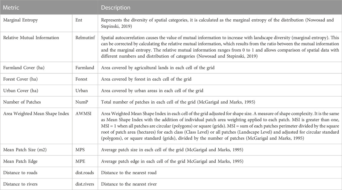
TABLE 1. Landscape metrics used to describe landscape structure surrounding recording sites in the Central Conservation Area of Costa Rica, 2019–2020.
2.3 Acoustic sampling
We sampled soundscapes in 91 recording sites in Grecia Forest Reserve and Poas Volcano National Park, and surroundings areas with productive activities (predominantly agricultural and urban). All recording sites were located in forest patches of at least 10 ha, inside or no more than 3 km away from protected areas (Figure 1).
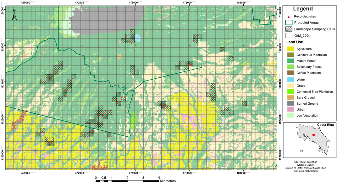
FIGURE 1. Study area in the Central Conservation Area of Costa Rica, 2019–2020.
We used Song Meter Digital Field Recorders (SM2 +; Wildlife Acoustics Inc, Supplementary Appendix S1) to sample soundscapes. Two omnidirectional microphones were placed in each recorder, so the recording would be made through two channels, or in stereo. A sampling rate or frequency rate of 44.1 kHz and 16 bits’ resolution were used. Audio files were recorded in Microsoft Wave (.wav) format. Audio files were stored on 64 GB capacity SDHC memory cards. At each recording site, the equipment was fixed to the trees at an approximate height of 1.50 m. The recorders were programmed to make continuous recordings during peaks of bird activity (4:00 a.m. - 7:00 a.m. and 15:00 p.m. - 18:00 p.m.), and for periods of 10 min every half an hour during the rest of the day. Acoustic recorders were active for a total of four to six consecutive days during the period July 2019 to June 2020.
2.4 Statistical analysis
2.4.1 Cluster analysis with landscape metrics
We ran a K-means cluster analysis (Hartigan & Wong Algorithm, 1979) to classify grid cells into clusters according to the landscape metrics described in Table 1. We selected the K-means method because it is one of the most used in this type of analysis and it has proven good results (Benocci et al., 2022). We specifically used marginal entropy (ent), relative mutual information (relmutinf), Farmland cover (Farmland), Forest cover (Forest), Urban cover (Urban), Mean Patch Edge (MPE), Number of patches (NumP), Area weight mean shape index (AWMSI) and Mean Patch Size (MPS) as classification variables (Table 1). We did not use the variables distance to roads and distance to rivers because this would have incorporated a spatial influence in the analysis and led to grouping the grid cells by their proximity rather than by the characteristics of the surrounding matrix. All variables were scaled to have mean = 0 and sd = 1. The optimal number of clusters was defined using the silhouette index (Rousseeuw, 1987).
2.4.2 Preselection of acoustic indices
Recordings were processed to obtain a series of 38 acoustic indices (Table 2) for every one-minute audio segment using packages Soundecology, version (1.3.3) (Villanueva-Rivera & Pijanowski, 2018) and Seewave, (version 2.0.5) (Sueur et al., 2008) for R (R Core Team 2020), and additional code developed by the Buxton et al. (2018). To reduce the number of indices for analysis, we evaluated the acoustic indices according to their performance to discriminate between clusters of grid cells classified using landscape variables. We ran a random forest classification model (Breiman 2001) using the median per hour and per cell of the grid of acoustic indices as explanatory variables to classify each grid cell into clusters. The percentage of importance of each index in the classification process was taken as a criterion to select acoustic indices for further analysis. We also eliminated the acoustic indices that were redundant or highly correlated and kept the indices that had demonstrated good performance as ecological indicators in other studies (Buxton et al., 2018; Eldridge et al., 2018; Ross et al., 2021). We finally reduced the set to 19 acoustic indices (Table 3), which represent a different characteristics of the sound, including entropy and acoustic diversity (ADI, AEI, Hf, Ht, TE, HvSPL, Hm), acoustic activity (ACI, AAdur, AAduranth, roughness), acoustic energy (BIO, NP, dif_L10L90, msldBA_low, MAE, mdBGL, NDSI) and dominant frequencies (dfreq).
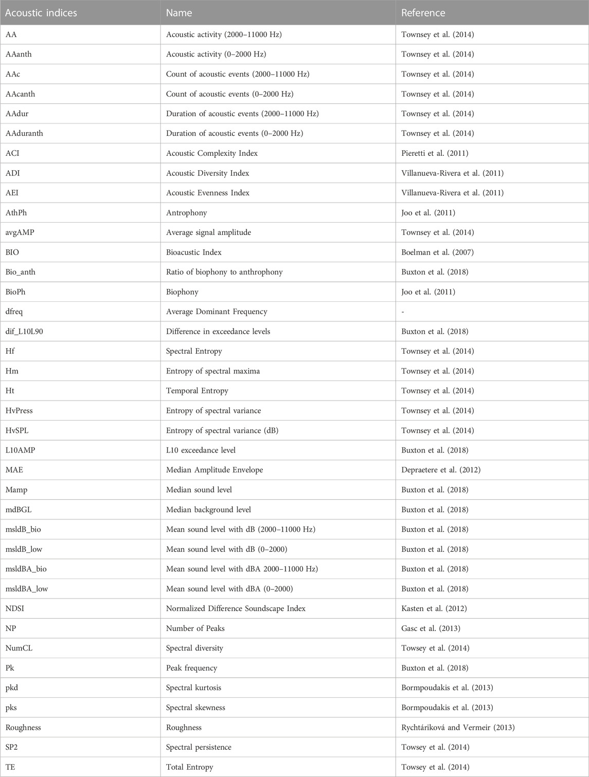
TABLE 2. Acoustic indices run initially for each sampling point in the Central Conservation Area of Costa Rica, 2019–2020.
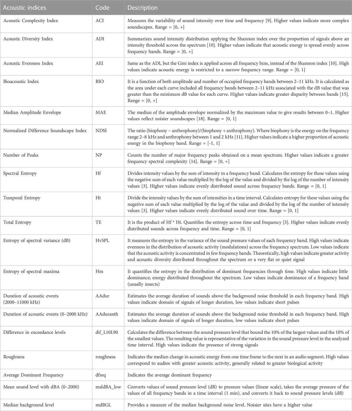
TABLE 3. Description of acoustic indices calculated for each sampling point in the Central Conservation Area of Costa Rica, 2019–2020.
We used the median per hour and per cell of the grid of every acoustic index for all analyses to avoid extreme values that may have occurred during a one-minute segment and to improve analysis performance. We manually listened and reviewed two recorders per site, for a total of 69331 min, labeling periods of heavy rain. We used this information to train a Random Forest model to predict the occurrence of heavy rain every minute according to the selected acoustic indices (Breiman 2001). Minute files containing heavy rain were not considered for further analyses.
2.4.3 Analysis of acoustic indices according to cluster created by the landscape metrics analysis
For evaluating the behavior and contrasting acoustic indices by clusters, we fitted generalized linear mixed-effects models using Template Model Builder (Brooks et al., 2017) using the median per hour and per cell of the grid of every acoustic index as the response variable while cluster, time (hour of the day), and the interaction between both, as fixed effects. The recorder ID was used as a random effect.
2.4.4 Analysis of dominant frequencies by cluster
We analyzed the dominance of each 1 kHz frequency band from 0–11 kHz according to clusters. Frequencies below 500 Hz were discarded to avoid bias in the dominant frequencies due to the self-noise of the recorder. Therefore, the first frequency band consisted of frequencies between 0.5–1 kHz. We performed generalized linear mixed-effects models (Maglianesi, 2016) for each frequency band using the hourly median of the number of times each frequency band was dominant as the response variable. The explanatory variables cluster, the hour of the day, and the interaction between the two were considered fixed effects. Recorder ID was taken as a random effect. The model also incorporated a zero-inflated formula, since the dominant frequency values had many zeros (for example, in all the minutes where a frequency band was not dominant). We first fitted models using Poisson distribution because the values of the dependent variable are integers (they represent counts of times in which the frequency band was dominant for every one-minute audio segment). However, this distribution generated an overdispersion, so a negative binomial distribution was finally used.
2.4.5 Modeling the relationship of acoustic indices with landscape metrics
We analyzed the relationship between acoustic indices and landscape metrics (ent, Forest, dist.rivers, dist.roads, NumP and MPE; Table 1). We did not used in this analysis other landscape metrics because they were highly correlated.
We performed generalized linear mixed-effects models to analyze the relationship between each acoustic indices and landscape variables. Models were fitted using the median per hour and per cell of the grid of every acoustic index as the response variable, the landscape metrics as independent fixed effects, and the recorder as a random effect. We included an autoregressive covariance structure (AR1) for hour of the day to account for potential temporal autocorrelation. Acoustic indices outliers were removed before analysis. Landscape metrics were standardized to improve model convergence.
We fitted NDSI, Hf, Ht, TE, MAE, Hm and HvSPL indices with beta error structure; NDSI was transformed before the analysis to convert its values between 0–1 using the formula (NDSI +1)/2 (Fairbrass et al., 2017). ACI, BIO, AAdur, AAduranth, dif_L10L90, roughness and dfreq were fitted using a gamma structure and log link function; ADI, msldBA_low and mdBGL with a Gaussian structure; and NP with a negative binomial structure as it is a count variable. Models were built using the R package glmmTMB (Brooks et al., 2017) and assumptions were checked using DHARMa package (Hartig, 2022).
2.4.6 Aural detection of biophonies and anthrophonies
A thorough review of the audio from 13 recorders was carried out aurally. We reviewed 10 min every half hour from 5:00 a.m. to 6:00 p.m. for three consecutive days in each recorder. The audios were searched for acoustic events, such as biophonies and anthrophonies, using the Adobe Audition program for listening and visualization. Biophonies were classified into taxonomic groups of birds, insects, amphibians, and mammals. We registered the duration in time (seconds) of each category of acoustic events for each hour of the day. We then summarized all categories into their mean and standard error per hour for comparison among clusters.
The distribution of the selected recorder was three from cluster 1, two from cluster 2, and eight from cluster 3. We used only birds and insects in the biophony category because mammals and amphibians were underrepresented in audio recordings.
3 Results
3.1 Cluster analysis with landscape metrics
The cluster analysis classified the sites into tree clusters (Figures 2, 3). Cluster 1 was characterized by more farmland and less forest cover, higher patch shape complexity, a higher number of patches, and the total edge. Cluster 2 and cluster 3 did not differ markedly regarding the amount of forest, however, cluster 2 presented more forest and less farmland cover than cluster 3. In addition, cluster 2 presented a lower number of patches, total edge, and patch shape complexity than the other clusters. Marginal entropy and relative mutual information did not differ between clusters (Figure 4; Table 4).
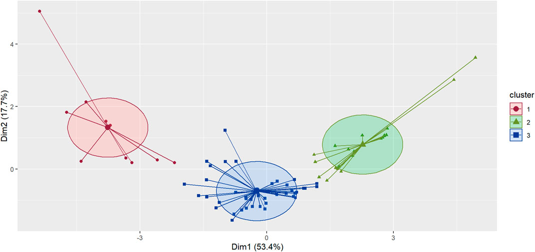
FIGURE 2. K-means cluster classification of sampling cells in the Central Conservation Area of Costa Rica, 2019–2020.
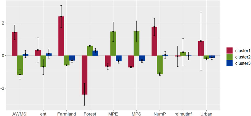
FIGURE 3. Geographic distribution of recording sites according to cluster classification created by the landscape metrics analysis.
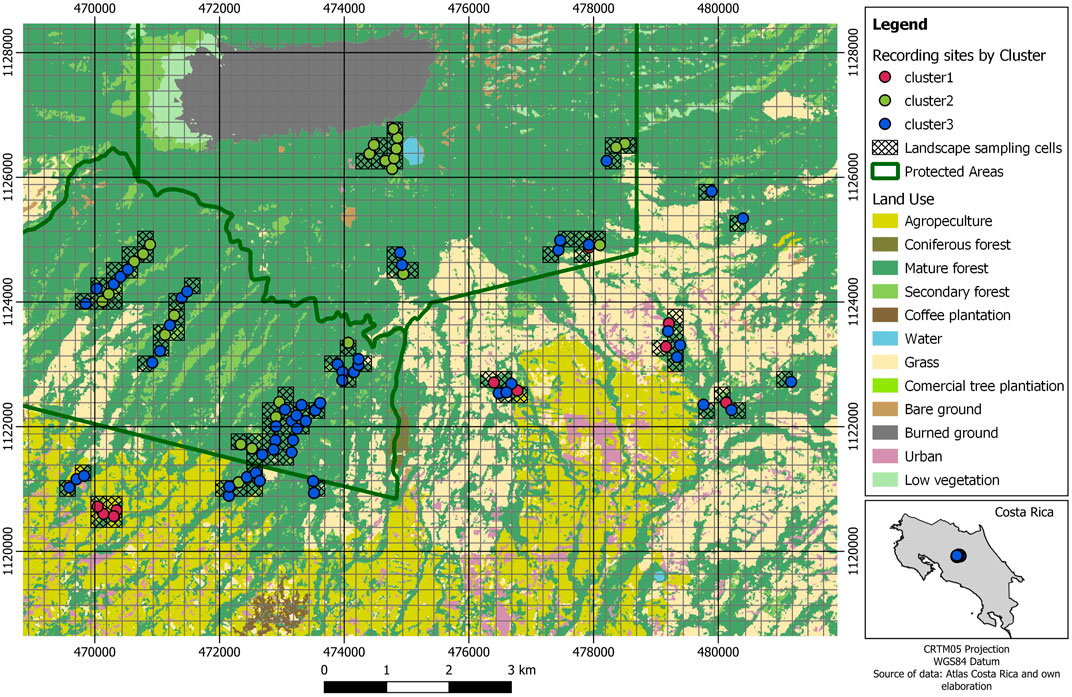
FIGURE 4. Mean values of the landscape variables for every cluster in the Central Conservation Area of Costa Rica, 2019–2020. Black lines represent the 95% confidence interval for the mean calculation. Y-axes represent the value of the scaled variable, where 0 represents the global mean for all values.
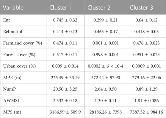
TABLE 4. Center values for every cluster and 95% confidence intervals in the Central Conservation Area of Costa Rica, 2019–2020.
3.2 Analysis of acoustic indices by cluster
To facilitate the interpretation, we present the results of the models showing the contrast between acoustic indices by cluster according to three categories of acoustic indices: 1) acoustic entropy and diversity indices (ADI, AEI, Hf, Ht, Hm, HvSPL, and TE) 2) acoustic activity or events indices (ACI, roughness, AADur, AADuranth, and NP), and 3) summary of acoustic energy indices (BIO, dif_L10L90, msldBA_low, MAE, mdBGL, NDSI and dfreq). In general, we observed a higher variability in all acoustic indices in cluster 1 than in clusters 2 and 3 (Figures 5–7).
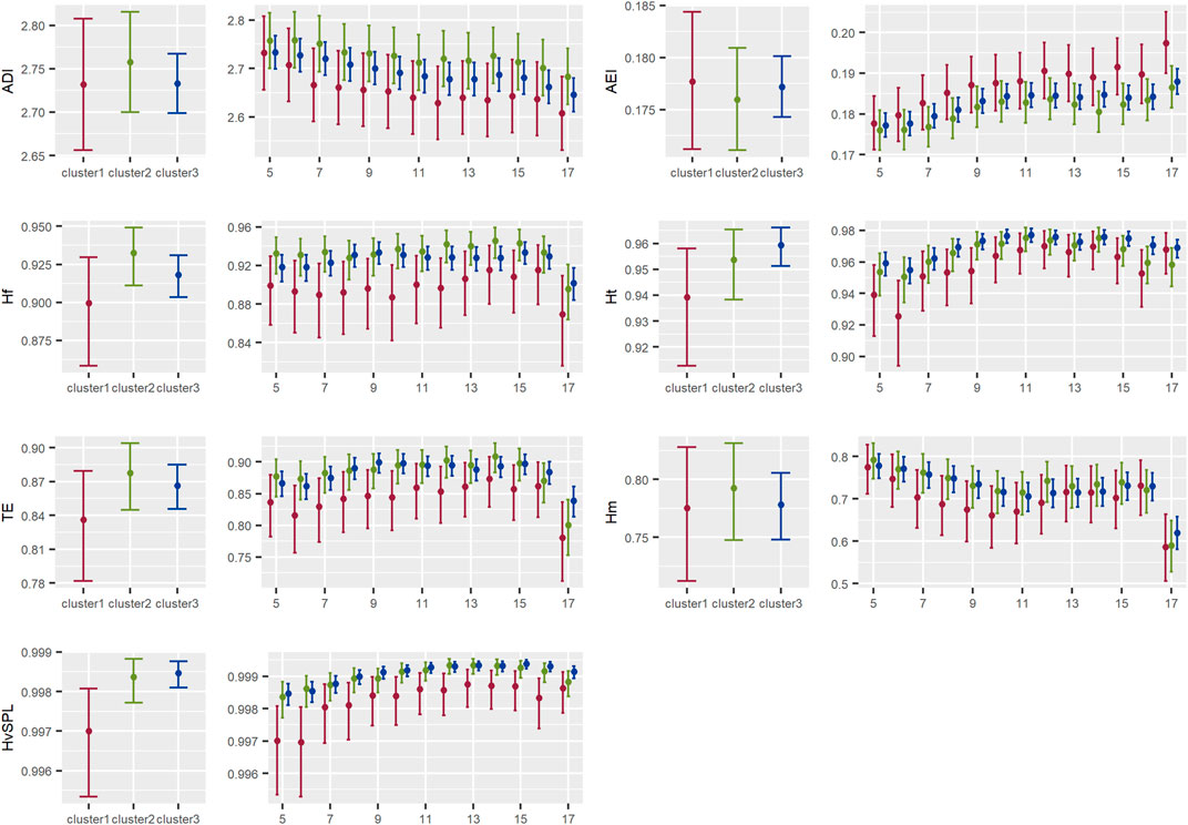
FIGURE 5. Results of the models showing the contrast between acoustic indices by cluster for the entropy and acoustic diversity type of indices in the Central Conservation Area of Costa Rica, 2019–2020.
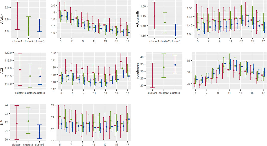
FIGURE 6. Results of the models showing the contrast between acoustic indices by cluster for the activity or acoustic events type of indices in the Central Conservation Area of Costa Rica, 2019–2020.
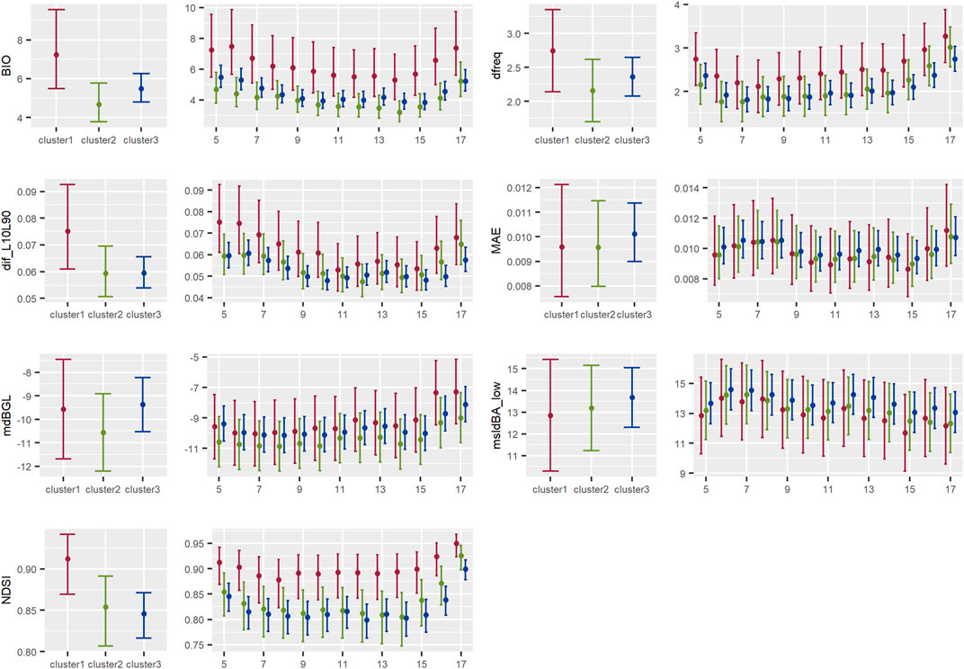
FIGURE 7. Results of the models showing the contrast between acoustic indices by cluster for the summary of acoustic energy indices type of indices in the Central Conservation Area of Costa Rica, 2019–2020.
3.2.1 Acoustic entropy and diversity indices
There was a general tendency, although statistically non-significant, of higher entropy or diversity in clusters 2 and 3 than in cluster 1, being more noticeable between clusters 2 and 1 in the afternoon hours. Following the opposite pattern, a lower AEI value (meaning a higher acoustic evenness) was detected in clusters 2 and 3 than in cluster 1. Besides, cluster 1 presented less variation in the variance of the energy among frequency bands than in clusters 2 and 3 (Figure 5).
3.2.2 Acoustic activity or events indices
There was a general tendency, although statistically non-significant, for a longer duration of sounds above the background noise threshold in each frequency band in cluster 1 than in clusters 2 and 3, both for the range of frequencies events between 0–2000 kHz and 2000–11000 kHz. On the other hand, acoustic complexity seemed to be higher in cluster 1 than in clusters 2 and 3; a contrasting result with roughness, given that both indices depict similar information about the acoustic activity. But, in general, none of the indices showed strong differences among clusters (Figure 6).
3.2.3 Summary of acoustic energy indices
As shown by BIO values, biological frequency bands in cluster 1 contained a higher amount of energy than cluster 2 during the day, although statistically non-significant for most hours, except at 6 a.m. The difference was not so notorious between clusters 1 and 3. This was reflected also in NDSI values, showing a higher proportion of acoustic energy in the biophony band in cluster 1 than in clusters 3 and 2, although less noticeable between clusters 2 and 3. Moreover, NDSI values were statistically significantly higher in cluster 1 than in cluster 3 at 6 a.m., 9 a.m., and from 2 p.m. to 5 p.m. There was a notorious increase in NDSI values in all clusters at 5 p.m. (Figure 7).
There also was a statistically non-significant tendency of higher dif_L10L90 values in cluster 1 than in clusters 3 and 2, which indicated the presence of stronger signals in cluster 1 than in the other clusters. A similar tendency was seen in the average dominant frequency, being higher (although statistically non-significant) in cluster 1 than 3 and 2 (Figure 7).
3.3 Analysis of dominant frequencies by cluster
The distribution of dominant frequencies between clusters was variable during the day (Figure 8). Low frequencies, from 0–1 kHz, were more dominant in cluster 2 than cluster 1 during all day, but only statistically significant at 17:00 p.m. The dominance of frequency bands between 1–4 kHz was similar in all clusters, except frequency band from 2–3 kHz, what was more dominant in cluster 1 than the other clusters, especially during the morning. Frequencies at intermediate level, from 4–7 kHz, were more dominant in cluster 1 than clusters 2 and 3. Mid-high frequency bands, from 7–9 kHz, presented a similar dominance across the three clusters. Higher frequencies, from 9–11 kHz, showed higher dominances in cluster 2 than the other clusters, what was most noticeable during the afternoon (Figure 8).
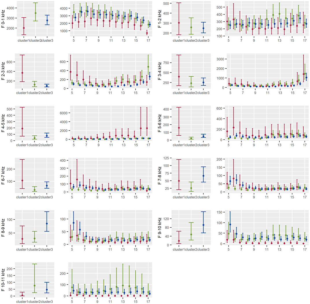
FIGURE 8. Distribution of dominant frequencies between clusters during the day in the Central Conservation Area of Costa Rica, 2019–2020.
3.4 Modeling the relationship of acoustic indices with landscape metrics
Landscape metrics had different effects on acoustic indices. Forest cover and distance to rivers were the variables that had a significant effect over more acoustic indices, followed by entropy (ent) and the number of patches (NumP). Distance to roads (dist.roads) and Mean patch edge (MPE) did not have a significant effect on any of the acoustic indices evaluated (Table 5; Supplementary Appendix S2).
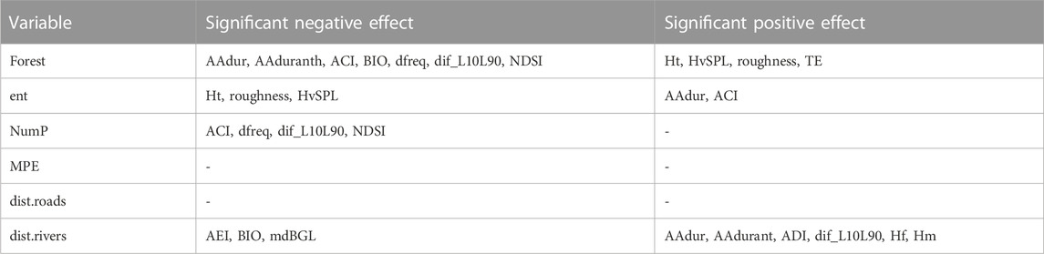
TABLE 5. Acoustic indices with a positive or negative statistically significant effect on each landscape variable in the Central Conservation Area of Costa Rica, 2019–2020.
There was a positive significant relationship between the amount of forest and acoustic entropy and diversity indices. However, sites with a higher amount of forest seemed to present a negative relationship with acoustic activity/events or acoustic energy summary type of indices. Accordingly, the higher the entropy at the landscape level, the lower the acoustic entropy, but the higher the acoustic activity/events (Table 5; Supplementary Appendix S2).
However, there was a negative relationship between the number of patches at the landscape level and acoustic energy summary indices. Distance to rivers also behaves in a counterintuitive way regarding acoustic indices, because the longer the distance from rivers, the higher acoustic diversity or entropy, as well as the duration and strength of signals (Table 5; Supplementary Appendix S2).
3.5 Aural detection of biophonies and anthrophonies
The mean duration (seconds) of biophonies per hour was higher in cluster 1 all day, followed by cluster 3 and cluster 2. This pattern was consistent when we analyzed only the sound produced by birds. The results for insects were similar between clusters in the morning, but cluster 2 and cluster 3 showed higher mean duration (seconds) of biophonies from insects in the afternoon. On the other hand, the mean duration (seconds) of anthrophonies was higher in the morning (5:00 a.m.-10:00 a.m.) and at 4:00 p.m. and 5:00 p.m. in cluster 1 than in the other clusters (Figure 9).
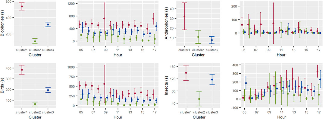
FIGURE 9. Distribution per hour of the mean time in one-minute segments occupied by biophonies (B1), birds (B2), insects (B3), and anthrophonies (B4) in every cluster. Lines represent 95% confidence intervals for the mean.
4 Discussion
Our study sites were classified according to a series of landscape metrics reflecting forest amount and fragmentation around the recording points, resulting in a more fragmented cluster (cluster 1), a more conserved cluster (cluster 2), and an intermediate cluster (cluster 3). We expected that more conserved sites would have, in general, greater acoustic diversity and activity, as well as a higher proportion of biophonies than antrophonies. The results were partially under these predictions. For example, we did find that there was a general tendency for higher acoustic entropy or diversity type of indices (for example Hf, Ht, Hm, HvSPL, and TE) in conserved (clusters 2 and 3) than in fragmented sites (cluster 1). Consequently, more conserved sites showed higher acoustic diversity, i.e. acoustic energy was more evenly distributed throughout the entire frequency spectrum. Moreover, more conserved sites presented more variation in the variance of the energy among frequency bands. These findings may reflect a higher diversity of species producing sounds in more conserved sites. Other authors have suggested that acoustic production might increase in diversity with different individuals and species vocalizing, resulting in more diverse acoustic communities in highly diverse communities in terms of the number of species and individuals (Sueur et al., 2014).
However, the opposite and unexpected pattern was found for acoustic activity (for instance ACI, AAdur, and Aaduranth) or summary of acoustic energy type of indices (BIO, NDSI, and dif_L10L90). For example, more conserved sites tended to present lower acoustic complexity, shorter duration of sounds above the background noise threshold for the range of frequencies events between 0–2 kHz and 2–11 kHz, and lower amount of energy in the biological frequency bands during the day. NDSI also followed the same pattern, given the relationship with the previous indices (BIO).
We additionally found a positive significant relationship between the amount of forest and acoustic entropy or diversity type of indices. However, sites with a higher amount of forest seemed to present a negative relationship with acoustic activity or energy type of indices. Moreover, the higher the entropy at the landscape level, the lower the acoustic entropy, but the higher the acoustic activity or energy. These results are consistent with other studies conducted by our group in the tropics (Retamosa Izaguirre et al., 2018; Retamosa Izaguirre et al., 2021a; Retamosa Izaguirre et al. et al., 2021b), providing support to our notion that, in the tropics, acoustic indices such as ACI and BIO seem to be indicating acoustic activity or energy rather than acoustic diversity, behaving as a weak or incomplete indicator of biodiversity or habitat conservation. In this sense, one or a few species with persistent vocal activity can result in high values of ACI or BIO, although the site might not be highly diverse or well conserved. However, acoustic entropy or diversity indices, such as Hf, Ht, HvSPL, and TE, might be more suitable to represent biodiversity and habitat conservation. In accordance, Do Nascimento et al. (2020) found that different habitat types had unique and predictable soundscapes; specifically, Ng et al. (2018) found a significant correlation between AEI, ADI, and H with a BioCondition Score that discriminated among woodland condition types, and Fuller et al. (2015) reported that AEI, H, and NDSI best reflected the soundscape with landscape characteristics, ecological condition, and bird species.
Consistently, the aural detection of biophonies showed that the mean duration in seconds of biophonies per hour was higher in cluster 1 (more fragmented) throughout the day, followed by cluster 3 (intermediate) and lastly cluster 2 (more conserved). These results were driven by birds, which replicated the same general pattern as biophonies. As indicated by other authors (Temple and Wiens, 1989; Niemi et al., 1997; Campos-Cerqueira et al., 2020), birds might not be the best indicator of habitat conservation, given the great plasticity and variety of life histories found in this group. There usually are some bird species that can take advantage of, or even benefit from, a certain degree of habitat alteration (Carrara et al., 2015). For instance, younger forests usually present a high environmental heterogeneity at horizontal and vertical levels (MacArthur and MacArthur, 1961), providing a variety of niches for some opportunistic species, or a mixture of species with different habitat requirements. Other authors have even indicated that forests at earlier stages of succession maintain a greater dynamic of food production than mature forests (Flores and Dezzeo, 2005), which may help increase the variety of species guilds inhabiting them (Almazán-Núñez et al., 2009). We highlight the importance of including other groups, for example, amphibians or insects as indicators of habitat conservation, or even using other parameters that measure behavior, activity, and overall condition or reproductive success for some selected wildlife species.
Regarding the mean duration (seconds) of anthrophonies, it was higher in the morning (5:00 a.m.-10:00 a.m.) and at 4:00 p.m. and 5:00 p.m. in cluster 1 (more fragmented) than in the other clusters. This is congruent with regular commercial activity, including the transit of service vehicles transporting goods and services, which tends to be more intense in the morning hours (Halfwerk et al., 2018). Besides, the peak in anthrophonies at 4:00 p.m. and 5:00 p.m. in cluster 1 might be associated with the transit of people returning home from regular-hour jobs. However, and how it was observed before, these changes in anthrophonies were not reflected in the NDSI index, given the higher energy in the biophony range detected in cluster 1, which also increased NDSI values. Nevertheless, both measures depict different information.
NDSI values reflect the ratio of the amount of energy between antrophony and biophony bands, while with the aural detection we measured the mean time where only anthrophonies were found on each one-minute segment of audio, regardless of the amount of energy. Therefore, if the anthrophonies had low energy, even if they were reflected in the aural analysis, they would not affect the NDSI index.
On the other hand, we found higher dominant frequencies in the more conserved and forested cluster (cluster 2), while intermediate frequencies dominated in the fragmented cluster (cluster 1). This might be due to the presence of species with persistent or loud vocalizations, resulting in dominant mid-frequencies in cluster 1 at specific periods, such as dawn and dusk, where the contrast in dominant frequencies between clusters was more noticeable. This idea is supported by the fact that we did not find evidence of higher acoustic diversity in cluster 1. Conversely, acoustic diversity seemed to be higher in cluster 2. Moreover, we suggest that conserved sites might be more acoustically diverse but quieter or with species less vocally active than fragmented sites.
Acoustic indices, as well as traditional indices in ecology, have the advantage of summarizing ecological information, but at the expense of not taking into account the composition of ecological communities (Izsák & Papp 2000). For this reason, we recommend combining information from acoustic indices with more specific acoustic or ecological information from selected species, that may serve as indicators of the pattern and process under investigation. However, acoustic entropy or diversity indices did behave well as indicators of habitat conservation or condition in this, as well as other studies (Fuller et al., 2015; Ng et al., 2018; Bradfer-Lawrence et al., 2020; Do Nascimento et al., 2020).
On a final note, the lack of statistical power to detect differences in acoustic indices among clusters might be due partially to the fine-scale landscape variability surrounding sampling sites. However, on a broad scale, sites were located mostly inside, near, or connected to big forest fragments included in protected areas (Volcan Poas National Park and Grecia Forest Reserve). Moreover, Costa Rica has conducted strong efforts to implement environmental services payment initiatives (Brownson et al., 2020), that in association with a strong ecotourism culture in the country, might have helped to maintain forest patches in the matrices around protected areas (Hunt & Harborpro 2019; Beita et al., 2021).
In conclusion, acoustic indices revealed that the surrounding matrices of protected areas have an impact on acoustic environments. Although disturbed environments with less-forested and more fragmented matrices registered higher values of acoustic energy and activity in certain biological frequency bands, sites with a higher percentage and more continuous forest cover showed higher values of acoustic entropy and diversity, reflecting a more diverse acoustic community. Given this pattern, we emphasize to researchers and decision-makers to carefully interpret acoustic indices when evaluating disturbed ecosystems showing a high value in acoustic energy or activity, because this might not accurately reflect a more biodiverse or conserved habitat. Finally, we highlight the importance of preserving undisturbed habitats with forested matrices, as they are important for maintaining acoustic diversity.
Data availability statement
The raw data supporting the conclusions of this article will be made available by the authors, without undue reservation.
Author contributions
Conceptualization, MR and JB; fieldwork, JB and MR; data analysis, JB and MR; writing of the manuscript, MR and JB. All authors have read and agreed to the published version of the manuscript.
Acknowledgments
We thank the staff of Grecia Forest Reserve and Poas Volcano National Park for their collaboration during fieldwork and the owners of the farms who allowed us access to data collection. We also thank the students of the National University who helped us in data collection and management (Marilyn Ureña Chaves, Gerardo Servellón Velado, Natalia Segura Vargas, Yanory Monge Fernández). We thank Manuel Spínola for the statistical analysis recommendations.
Conflict of interest
The authors declare that the research was conducted in the absence of any commercial or financial relationships that could be construed as a potential conflict of interest.
Publisher’s note
All claims expressed in this article are solely those of the authors and do not necessarily represent those of their affiliated organizations, or those of the publisher, the editors and the reviewers. Any product that may be evaluated in this article, or claim that may be made by its manufacturer, is not guaranteed or endorsed by the publisher.
Supplementary material
The Supplementary Material for this article can be found online at: https://www.frontiersin.org/articles/10.3389/frsen.2023.1051555/full#supplementary-material
References
Almazán-Núñez, R., Puebla-Olivares, F., and Almazán-Juárez, Á. (2009). Diversidad de Aves en Bosques de Pino-Encino del Centro de Guerrero, México. Acta Zoológica Mex. (N.S.) 25 (1), 123–142. doi:10.21829/azm.2009.251604
Barber, J. R., Burdett, C. L., Reed, S. E., Warner, K. A., Formichella, C., Crooks, K. R., et al. (2011). Anthropogenic noise exposure in protected natural areas: Estimating the scale of ecological consequences. Landsc. Ecol. 26, 1281–1295. doi:10.1007/s10980-011-9646-7
Beita, C. M., Murillo, L. F. S., and Alvarado, L. D. A. (2021). Ecological corridors in Costa Rica: An evaluation applying landscape structure, fragmentation-connectivity process, and climate adaptation. Conservation Sci. Pract. 3 (8), e475. doi:10.1111/csp2.475
Benocci, R., Potenza, A., Bisceglie, A., Roman, H. E., and Zambon, G. (2022). Mapping of the acoustic environment at an urban Park in the city area of milan, Italy, using very low-cost sensors. Sensors 22 (9), 3528. doi:10.3390/s22093528
Boelman, N. T., Asner, G. P., Hart, P. J., and Martin, R. E. (2007). Multi-trophic invasion resistance in Hawaii: Bioacoustics, field surveys, and airborne remote sensing. Ecol. Appl. 17, 2137–2144. doi:10.1890/07-0004.1
Bormpoudakis, D., Sueur, J., and Pantis, J. (2013). Spatial heterogeneity of ambient sound at the habitat type level: Ecological implications and applications. Landsc. Ecol. 28, 495–506. doi:10.1007/s10980-013-9849-1
Bradfer-Lawrence, T., Bunnefeld, N., Gardner, N., Willis, S. G., and Dent, D. H. (2020). Rapid assessment of avian species richness and abundance using acoustic indices. Ecol. Indic. 115, 106400. doi:10.1016/j.ecolind.2020.106400
Brooks, M. E., Kristensen, K., van Benthem, K. J., Magnusson, A., Berg, C. W., Nielsen, A., et al. (2017). glmmTMB balances speed and flexibility among packages for zero-inflated generalized linear mixed modeling. R J. 9 (2), 378–400. doi:10.32614/rj-2017-066
Brownson, K., Anderson, E. P., Ferreira, S., Wenger, S., Fowler, L., and German, L. (2020). Governance of Payments for Ecosystem Ecosystem services influences social and environmental outcomes in Costa Rica. Ecol. Econ. 174, 106659. doi:10.1016/j.ecolecon.2020.106659
Buxton, R. T., McKenna, M. F., Clapp, M., Meyer, E., Stabenau, E., Angeloni, L. M., et al. (2018). Efficacy of extracting indices from large-scale acoustic recordings to monitor biodiversity. Conserv. Biol. 32 (5), 1174–1184. doi:10.1111/cobi.13119
Campos-Cerqueira, M., Mena, J., Tejeda-Gómez, V., Aguilar-Amuchástegui, N., Gutiérrez, N., and Mitchell Aide, T. (2020). How does FSC forest certification affect the acoustically active fauna in Madre de Dios, Peru? Remote Sens. Ecol. Conservation 6 (3), 274–285. doi:10.1002/rse2.120
Carrara, E., Arroyo-Rodríguez, V., Vega-Rivera, J. H., Schondube, J. E., de Freitas, S. M., and Fahrig, L. (2015). Impact of landscape composition and configuration on forest specialist and generalist bird species in the fragmented Lacandona rainforest, Mexico. Biol. Conserv. 184, 117–126. doi:10.1016/j.biocon.2015.01.014
Depraetere, M., Pavoine, S., Jiguet, F., Gasc, A., Duvail, S., and Sueur, J. (2012). Monitoring animal diversity using acoustic indices: Implementation in a temperate woodland. Ecol. Indic. 13 (1), 46–54. doi:10.1016/j.ecolind.2011.05.006
Do Nascimento, L., Campos-Cerqueira, M., and Bearda, K. (2020). Acoustic metrics predict habitat type and vegetation structure in the Amazon. Ecol. Indic. 117, 106679. doi:10.1016/j.ecolind.2020.106679
Eldridge, A., Guyot, P., Moscoso, P., Johnston, A., Eyre-Walker, Y., and Peck, M. (2018). Sounding out ecoacoustic metrics: Avian species richness is predicted by acoustic indices in temperate but not tropical habitats. Ecol. Indic. 95, 939–952. doi:10.1016/j.ecolind.2018.06.012
ESRI (2016). ArcGIS desktop: Release 10.5. Redlands, California, USA: Environmental Systems Research Institute.
Fahrig, L. (2003). Effects of habitat fragmentation on biodiversity. Annu. Rev. Ecol. Evol. Syst. 34, 487–515. doi:10.1146/annurev.ecolsys.34.011802.132419
Fairbrass, A. J., Rennett, P., Williams, C., Titheridge, H., and Jones, K. E. (2017). Biases of acoustic indices measuring biodiversity in urban areas. Ecol. Indic. 83, 169–177. doi:10.1016/j.ecolind.2017.07.064
Farina, A., Pieretti, N., and Piccioli, L. (2011). The soundscape methodology for long-term bird monitoring: A mediterranean europe case-study. Ecol. Inf. 6, 354–363. doi:10.1016/j.ecoinf.2011.07.004
Flores, S., and Dezzeo, N. (2005). Variaciones temporales en cantidad de semillas en el suelo y en lluvia de semillas en un gradiente bosque-sabana en la Gran Sabana, Venezuela. Interciencia 30 (1), 39–43.
Fuller, S., Axel, A. C., Tucker, D., and Gage, S. H. (2015). Connecting soundscape to landscape: Which acoustic index best describes landscape configuration? Ecol. Indic. 58, 207–215. doi:10.1016/j.ecolind.2015.05.057
Gasc, A., Sueur, J., Pavoine, S., Pellens, R., and Grandcolas, P. (2013). Biodiversity sampling using a global acoustic approach: Contrasting sites with microendemics in New Caledonia. PloS one 8 (5), e65311. doi:10.1371/journal.pone.0065311
Glaser, G. (2015). Strengthening the scientific evidence base of a new climate agreement. Ecosyst. Health Sustain. 1 (9), 1–4. doi:10.1890/EHS15-0034.1
González, F., Seas, C., Barrientos, Z., Quesada-Acuña, S. G., and Mora Amador, R. A. (2019). in The pulsing heart of Central America volcanic zone, 309–317.Poás Volcano Biodiversity. Poás Volcano
Halfwerk, W., Lohr, B., and Slabbekoorn, H. (2018). “Impact of man-made sound on birds and their songs,” in Effects of anthropogenic noise on animals. Editors H. Slabbekoorn, R. J. Dooling, and N. Popper (Berlin, Germany: Springer), 209–242. doi:10.1007/978-1-4939-8574-6_8
Hartig, F. (2022). “Package ‘DHARMa’,” in Residual Diagnostics for Hierarchical (Multi-Level/Mixed) Regression Models. Version 0.4.6. Available at: http://florianhartig.github.io/DHARMa/.
Hartigan, J. A., Wong, M. A., and Algorithm, A. S. (1979). Algorithm as 136: A K-means clustering Algorithm. Appl. Stat. 28, 100–108. doi:10.2307/2346830
Hesselbarth, M. H., Sciaini, M., With, K. A., Wiegand, K., and Nowosad, J. (2019). landscapemetrics: an open-source R tool to calculate landscape metrics. Ecography 42, 1648–1657. doi:10.1111/ecog.04617
Hunt, C. A., and HarborPro, L. C. (2019). Pro-environmental tourism: Lessons from adventure, wellness and eco-tourism (AWE) in Costa Rica. J. Outdoor Recreat. Tour. 28, 28. doi:10.1016/j.jort.2018.11.007
Izsák, J., and Papp, L. (2000). A link between ecological diversity indices and measures of biodiversity. Ecol. Model. 130 (1-3), 151–156. doi:10.1016/S0304-3800(00)00203-9
Joo, W., Gage, S. H., and Kasten, E. P. (2011). Analysis and interpretation of variability in soundscapes along an urban-rural gradient. Landsc. Urban Plan. 103, 259–276. doi:10.1016/j.landurbplan.2011.08.001
Kasten, E. P., Fox, S. H. Gage J., and Joo, W. (2012). The remote environmental assessment laboratory's acoustic library: An archive for studying soundscape ecology. Ecol. Inf. 12, 50–67. doi:10.1016/j.ecoinf.2012.08.001
Leandro, O. V., Vargas, R., and Ramírez, M. R. (2016). Plan general de Manejo de la Reserva forestal Grecia 2016 - 2023. Available at: https://www.sinac.go.cr/ES/planmanejo/Plan%20Manejo%20ACC/Reserva%20Forestal%20Grecia.pdf.
Macarthur, R. H., and Macarthur, J. W. (1961). On bird species diversity. Ecology 42 (3), 594–598. doi:10.2307/1932254
Machado, R. B., Aguiar, L., and Jones, G. (2017). Do acoustic indices reflect the characteristics of bird communities in the savannas of Central Brazil. Landsc. Urban Plan. 162, 36–43. doi:10.1016/j.landurbplan.2017.01.014
Maglianesi, M. (2010). Avifauna asociada al bosque nativo y plantación exótica de coníferas en la Reserva Forestal Grecia, Costa Rica. Ornitol. Neotropical 21 (3), 339–350.
Maglianesi, M. (2016). Factores que afectan la Reserva Forestal Grecia (Alajuela, Costa Rica) disminuyendo su valor para la conservación de la biodiversidad. Biocenosis 23 (1).
Mammides, C., Goodaleb, E., Dayananda, S. K., Kang, L., and Chen, J. (2017). Do acoustic indices correlate with bird diversity? Insights from two biodiverse regions in yunnan province, south China. Ecol. Indic. 82, 470–477. doi:10.1016/j.ecolind.2017.07.017
Marsh, D. M., and Trenham, P. C. (2008). Current trends in plant and animal population monitoring. Conserv. Biol. 22 (3), 647–655. doi:10.1111/j.1523-1739.2008.00927.x
Maxwell, S., Cazalis, V., Dudley, N., Hoffmann, M., Rodrigues, A., Stolton, S., et al. (2020). Area-based conservation in the twenty-first century. Nature 586 (8), 217–227. doi:10.1038/s41586-020-2773-z
McGarigal, K., and Marks, B. J. (1995). FRAGSTATS: Spatial pattern analysis program for quantifying landscape structure. USDA Forest Service General Technical Report PNW-351, Corvallis. doi:10.4236/oje.2012.23019
Naoki, K. F., Durán, J., and Sánchez, J. E. (2003). La avifauna de un fragmento de bosque secundario en el Valle central, Costa Rica: Su estacionalidad e implicación para la conservación. Rev. Brenesia 59-60, 49–64.
Napoletano, B. (2004). Measurement, quantification and interpretation of acoustic signals within an ecological context. United States: Michigan State University. [master’s thesis]. [East Lansing (MI)].
Ng, M., Butler, N., and Woods, N. (2018). Soundscapes as a surrogate measure of vegetation condition for biodiversity values: A pilot study. Ecol. Indic. 93, 1070–1080. doi:10.1016/j.ecolind.2018.06.003
Niemi, G. J., Hanowski, J. M., Lima, A. R., Nicholls, T., and Weiland, N. (1997). A critical analysis on the use of indicator species in management. J. Wildl. Manag. 61, 1240–1251. doi:10.2307/3802123
Noches, L. (2005). Actualización de la evaluación de los recursos forestales mundiales. Informe del país Costa Rica, Programa de los recursos Forestales mundiales, Organización de las Naciones Unidas para la Agricultura y la Alimentación. Roma, Italia: FAO.
Nowosad, J., and Stepinsk, T. F. (2019). Information theory as a consistent framework for quantification and classification of landscape patterns. Landscape Ecol. 34, 2091–2101. doi:10.1007/s10980-019-00830-x
Pieretti, N., Duarte, M. H., Sousa-Lima, R. S., Rodrigues, M., Young, R. J., and Farina, A. (2015). Determining temporal sampling schemes for passive acoustic studies in different tropical ecosystems. Trop. Conservation Sci. 8 (1), 215–234. doi:10.1177/194008291500800117
Pieretti, N., Farina, A., and Morri, D. (2011). A new methodology to infer the singing activity of an avian community: The acoustic complexity index (ACI). Ecol. Indic. 11, 868–873. doi:10.1016/j.ecolind.2010.11.005
Pijanowski, B., Villanueva-Rivera, L. J., Dumyahn, S. L., Farina, A., Krause, B. L., Napoletano, B. M., et al. (2011). Soundscape ecology: The science of sound in the landscape. Bioscience 61 (3), 203–216. doi:10.1525/bio.2011.61.3.6
Pimm, S. L., Jenkins, C. N., and Li, B. V. (2018). How to protect half of Earth to ensure it protects sufficient biodiversity. Sci. Adv. 4 (8), eaat2616. doi:10.1126/sciadv.aat2616
Qi, J., Gage, S. H., Joo, W., Napoletano, B., and Biswas, S. (2008). “Soundscape characteristics of an environment: A new ecological indicator of ecosystem health,” in Wetland and water resource modeling and assessment: A watershed perspective. Editor W. Ji (Boca Raton, Florida, USA: CRC Press), 201–211.
R Core Team (2020). R: A language and environment for statistical computing. Vienna, Austria: R Foundation for Statistical Computing. [software] (Version 3.6.
Retamosa Izaguirre, M. I., Barrantes-Madrigal, J., Segura Sequeira, D., Spínola-Parallada, M., and Ramírez-Alán, O. (2021b). It is not just about birds: What acoustic indices reveal about a Costa Rican tropical rainforest? Neotropical Biodivers. 7 (1), 431–442. doi:10.1080/23766808.2021.1971042
Retamosa Izaguirre, M. I., Ramírez-Alán, O., and De la O Castro, J. (2018). Acoustic indices applied to biodiversity monitoring in a Costa Rica dry tropical forest. J. Ecoacoustics 2, 5. #TNW2NP. doi:10.22261/JEA.TNW2NP
Retamosa-Izaguirre, M. I., Segura-Sequeira, D., Barrantes-Madrigal, J., Spínola-Parallada, M., and Ramírez-Alán, O. (2021a). Vegetation, bird and soundscape characterization: A case study in braulio carrillo national Park, Costa Rica. Biota Colomb. 22 (1), 57–73. doi:10.21068/c2021.v22n01a04
Rodríguez, A., Gasc, A., Pavoine, S., Grandcolas, P., Gaucher, P., and Sueur, J. (2014). Temporal and spatial variability of animal sound within a neotropical forest. Ecol. Inf. 21, 133–143. doi:10.1016/j.ecoinf.2013.12.006
Ross, S. R. P-J., Friedman, N. R., Yoshimura, M., Yoshida, T., Donohue, I., and Economo, E. P. (2021). Utility of acoustic indices for ecological monitoring in complex sonic environments. Ecol. Indic. 121, 107114. doi:10.1016/j.ecolind.2020.107114
Rousseeuw, P. (1987). Silhouettes: A graphical aid to the interpretation and validation of cluster analysis. J. Comput. Appl. Math. 20, 53–65. doi:10.1016/0377-0427(87)90125-7
Rychtáriková, M., and Vermeir, G. (2013). Soundscape categorization on the basis of objective acoustical parameters. Appl. Acoust. 74, 240–247. doi:10.1016/j.apacoust.2011.01.004
Schafer, R. M. (1977). The soundscape: Our sonic environment and the tuning of the world. Rochester, Vermont, USA: Destiny Books.
Silhouettes, R. P. J. (1987). Silhouettes: A graphical aid to the interpretation and validation of cluster analysis. J. Comput. Appl. Math. 20, 53–65. doi:10.1016/0377-0427(87)90125-7
Sinac, V. (2014). Informe Nacional al Convenio sobre la Diversidad Biológica. San José, Costa Rica: GEF-PNUD.
Sueur, J., Farina, A., Gasc, A., Pieretti, N., and Pavoine, S. (2014). Acoustic indices for biodiversity assessme nt and landscape investigation. Acta Acustica United Acustica 100, 772–781. doi:10.3813/AAA.918757
Sueur, J., Pavoine, S., Hamerlynck, O., and Duvail, S. (2008). Rapid acoustic survey for biodiversity appraisal. PLoS One 3, e4065. doi:10.1371/journal.pone.0004065
Temple, S. A., and Wiens, J. A. (1989). Bird populations and environmental changes: Can birds be bio-indi¬cators? Am. Birds 43, 260–270.
Towsey, M., Wimmer, J., Williamson, I., and Roe, P. (2014). The use of acoustic indices to determine avian species richness in audio-recordings of the environment. Ecol. Inf. 21, 110–119. doi:10.1016/j.ecoinf.2013.11.007
Trigg, L. (2015). Assessment of acoustic indices for monitoring phylogenetic and temporal patterns of biodiversity in tropical forests. London (England)]: Imperial College London. [dissertation].
Villanueva-Rivera, L. J., Pijanowski, B. C., Doucette, J., and Pekin, B. (2011). A primer of acoustic analysis for landscape ecologists. Landsc. Ecol. 26 (9), 1233–1246. doi:10.1007/s10980-011-9636-9
Keywords: acoustic indices, soundscape, habitat conservation, biodiversity, landscape metrics
Citation: Retamosa Izaguirre M and Barrantes Madrigal J (2023) Soundscape structure in forests surrounded by protected and productive areas in central Costa Rica. Front. Remote Sens. 4:1051555. doi: 10.3389/frsen.2023.1051555
Received: 22 September 2022; Accepted: 27 February 2023;
Published: 09 March 2023.
Edited by:
Bryan Christopher Pijanowski, Purdue University, United StatesReviewed by:
Zhao Zhao, Nanjing University of Science and Technology, ChinaGiovanni Zambon, University of Milano-Bicocca, Italy
Andrey Atemasov, V. N. Karazin Kharkiv National University, Ukraine
Copyright © 2023 Retamosa Izaguirre and Barrantes Madrigal. This is an open-access article distributed under the terms of the Creative Commons Attribution License (CC BY). The use, distribution or reproduction in other forums is permitted, provided the original author(s) and the copyright owner(s) are credited and that the original publication in this journal is cited, in accordance with accepted academic practice. No use, distribution or reproduction is permitted which does not comply with these terms.
*Correspondence: Mónica Retamosa Izaguirre, bXJldGFtb3NAdW5hLmNy