 Yogita Karale
 May Yuan
- Geospatial Information Sciences, the University of Texas at Dallas, Richardson, TX, United States
Fine particulate matter, also known as PM2.5, has many adverse impacts on human health. However, there are few ground monitoring stations measuring PM2.5. Satellite data help fill the gaps in ground measurements, but most studies focus on estimating daily PM2.5 levels. Studies examining the effects of environmental exposome need accurate PM2.5 estimates at fine temporal intervals. This work developed a Convolutional Neural Network (CNN) to estimate the PM2.5 concentration at an hourly average using high-resolution Aerosol Optical Depth (AOD) from the MODIS MAIAC algorithm and meteorological data. Satellite-acquired AOD data are instantaneous measurements, whereas stations on the ground provide an hourly average of PM2.5 concentration. The current work aimed to refine PM2.5 estimates at temporal intervals from 24-h to 1-h averages. Our premise posited the enabling effects of spatial convolution on temporal refinements in PM2.5 estimates. We trained a CNN to estimate PM2.5 corresponding to the hour of AOD acquisition in the Dallas-Fort Worth and surrounding area using 10 years of data from 2006–2015. The CNN accepts images as input. For each PM2.5 station, we strategically subset temporal MODIS images centering at the PM2.5 station. Hence, the resulting image-patch size represented the size of the area around the PM2.5 station. It thus was analogous to spatial lag in spatial statistics. We systematically increased the image-patch size from 3 × 3, 5 × 5, … , to 19 × 19 km2 and observed how increasing the spatial lag impacted PM2.5 estimation. Model performance improved with a larger spatial lag; the model with a 19 × 19 km2 image-patch as input performed best, with a correlation coefficient of 0.87 and a RMSE of 2.57 g/m3 to estimate PM2.5 at in situ stations corresponding to the hour of satellite acquisition time. To overcome the problem of a reduced number of image-patches available for training due to missing AOD, the study employed a data augmentation technique to increase the number of samples available to train the model. In addition to avoiding overfitting, data augmentation also improved model performance.
1 Introduction
The Global Burden Disease study reported that air pollution caused 4.2 million deaths in 2015 due to particulate matter (Cohen et al., 2017). In addition, recent studies found a link between PM2.5 and several neurological disorders like dementia, Alzheimer’s, and Parkinson’s diseases (Kioumourtzoglou et al., 2016; Chen et al., 2017). Despite the harmful effects of PM2.5 on health, ground monitoring stations providing information about PM2.5 concentration are considerably sparse and unsuitable for spatial interpolation at a local scale. As a result, interpolations of PM2.5 from the nearest available monitoring stations to estimate the exposure in epidemiological studies are likely unreliable due to the underestimation of spatial variability in PM2.5 (Özkaynak et al., 2013). In an effort to overcome sparse measurements from ground stations, satellite-derived PM2.5 is widely used. These efforts focus on estimating daily PM2.5 levels. However, PM2.5 data over finer temporal intervals are necessary for accurate environmental exposure estimation. This study explores the use of satellite data to estimate PM2.5 over a temporal interval of 1 h in contrast to daily PM2.5 levels.
A common approach to characterize the spatial distribution of PM2.5 utilizes satellite-based Aerosol Optical Depth (AOD) as one of the predictor variables (Chudnovsky et al., 2014; Lary et al., 2014; Xie et al., 2015; Guo et al., 2017). AOD measures the amount of aerosols present in the atmosphere according to the optical properties of aerosols in an atmospheric column. However, the relationship between PM2.5 and AOD is complicated. AOD is affected by the size of the particles, the type of the particles, and meteorological factors. Depending on the source, the composition of the particles may vary in space and time (Bell et al., 2007). Meteorological factors (such as cloud fraction, relative humidity, temperature, boundary layer height, wind speed, and others) also affect this relationship (Lary et al., 2014; Guo et al., 2017). Several studies report PM2.5-AOD relationship varies with geography (Engel-Cox et al., 2004), time (Guo et al., 2017), the scale of regional or local studies (Chudnovsky et al., 2014), and AOD data resolution (Chudnovsky et al., 2014; Xie et al., 2015; Guo et al., 2017). Therefore, empirical models using AOD to estimate PM2.5 developed for one geographical area cannot be used for others.
The limited number of air quality stations in a geographical area may not meet the sample size requirements of parametric statistical frameworks, such as multiple linear regression. As a general rule of thumb, a multiple linear regression requires a minimum of 30 observations. Thus, these approaches are unsuitable in areas with sparse monitoring stations. Low-cost sensors such as PurpleAir (https://www2.purpleair.com/) have been deployed in large numbers across the United States. While these low-cost sensors help reduce the gap in spatial coverage of PM2.5 measurements, the accuracy of these sensors remains a cause of concern. A field evaluation of three PurpleAir sensors carried out at Rubidoux Air Monitoring Station in California for 2 months indicates that, in general, PurpleAir sensors can show an overall trend of PM2.5 within a day and across days but tend to overestimate PM2.5 concentration most of the times (Gupta et al., 2018). Specifically, the California study highlights that the bias of PurpleAir sensors increases with rising PM2.5 concentration. Moreover, PurpleAir sensors’ observations deviate from 0% to 90% of their hourly mean values.
A specification error due to the incorrect functional form between dependent and independent variables leads to biases in estimation (Ramsey, 1969), and proper relationship specifications are challenging for PM2.5 models using AOD (Lary et al., 2014). In-situ stations measure PM2.5 as the ground-level concentration of particles with an aerodynamic diameter less than 2.5 micrometers. In contrast, AOD measures the extinction of light due to aerosols in the atmospheric column (Nam et al., 2018). AOD and PM2.5 are independently affected by meteorological parameters (Guo et al., 2017), further complicating their relationship. Furthermore, AOD is an instantaneous measurement from space, and PM2.5 is an hourly average measured in situ at respective ground monitoring stations. Researchers proposed diverse modeling approaches to overcome the complicated relationship but lacked sufficient attention to the differences in temporal representations of AOD and PM2.5.
Literature reported several approaches to model the PM2.5-AOD relationship, like land-use regression (Lee, 2019), geographically weighted regression (Hu et al., 2013; van Donkelaar et al., 2015), back propagation artificial neural network (Gupta and Christopher, 2009a), mixed effect models (Xie et al., 2015), linear regression models (Gupta and Christopher, 2009b), and chemical transport models (Geng et al., 2015). The mixed effect modeling approach appeared popular among these approaches to 24-h average PM2.5 estimation. Some studies used AOD as the only predictor (Chudnovsky et al., 2014; Xie et al., 2015); others included additional parameters to improve model performance (Hu et al., 2014; Stafoggia et al., 2017). Xie et al. (2015) used a mixed effect model to account for spatiotemporal variations in PM2.5-AOD relationship with day-specific and site-specific parameters for AOD. Moreover, several other studies implemented similar mixed effect models by including AOD and additional spatiotemporal parameters (Hu et al., 2014; Stafoggia et al., 2017). In addition to day-specific random parameters, Stafoggia et al. (2017) introduced region-specific random parameters to account for variation in PM10-AOD relations across different regions in Italy. In the Southeastern United States, Hu et al. (2014) used a mixed effect model to capture temporal variability in the PM2.5-AOD relationship and followed with Geographically Weighted Regression on the residuals to account for spatial variability. Spatial and temporal parameters considered in these studies include population density, emission data, elevation, land cover, road density, Normalized Difference Vegetation Index (NDVI), meteorological data, etc. Zheng et al. (2013) applied a deep learning framework to predict the hourly Air Quality Index (AQI) for Beijing at 1 km resolution with region-specific parameters representative of traffic features (e.g., mean, standard deviation, and distribution of speeds on the road) and human mobility features (e.g., number of people arriving and departing a location). Such region-specific parameters may not be available or appropriate for areas outside Beijing.
Machine learning recently gained traction in modeling PM2.5 (Lary et al., 2014; Di et al., 2016; Hu et al., 2017; Li et al., 2017; Park et al., 2020). Several of these studies incorporated spatial dependence in the machine learning methods. Di et al. (2016) used an artificial neural network (ANN) for the northeastern United States to calibrate PM2.5 obtained from a chemical transport model, and Li et al. (2017) used the deep belief network approach to estimate PM2.5 in China. They considered spatial and temporal autocorrelation using lagged spatial and temporal terms. Spatial lag was incorporated by using PM2.5 measurements from nearby stations weighted by the inverse of their distance from the monitor under consideration, hence, essentially the classic spatial interpolation based on inverse distance weighting. An alternative way of applying weights in PM2.5 estimation was the boosting technique in machine learning. Boosting gave more weight to observations with high errors to improve model performance. Zhan et al. (2017) used geographically weighted gradient boosting to account for spatial non-stationarity in PM2.5 and AOD as well as meteorological factors. These methods refine the spatial resolution of PM2.5 estimation but retain temporal resolution at daily averages.
Advances in deep learning opened opportunities to convolute in situ and satellite observations for PM2.5 estimation. Park et al. (2020) used a convolutional neural network (CNN) to estimate the 24-h averaged PM2.5 across the conterminous United States using the 1-year data from 2011. Hu et al. (2017) incorporated inverse distance weighted PM2.5 from nearby stations as input to the random forest model. Clouds or high surface brightness might obscure AOD data from MODIS. Due to the high missing rate of AOD, both studies applied the GEOS-Chem model to simulate AOD data; Hu et al. (2017) used GEOS-Chem AOD when MODIS AOD was missing, whereas Park et al. (2020) used both MODIS AOD and GEOS-Chem AOD. Along with the AOD data, both studies used meteorological data, land-use variables, and National Emission Inventory (NEI) data as predictors. Several data issues were prominent in both studies. NEI database provided information about pollutant-wise emissions at annual scales. However, methods used to estimate these emissions might vary from year to year (U.S. Environmental Protection Agency, 2020). Therefore, the data from these emission inventories were unsuitable for multi-year studies. Land-use data were static and could contribute very little in explaining hourly PM2.5 variation. Li et al. (2017) reported that the inclusion of road networks as one of the predictors showed a minimal impact on model performance, whereas population worsened the model performance. Furthermore, in areas with sparsely distributed monitoring stations, a model developed with land-use and population density around very few monitoring stations might not be representative enough to allow model generalizability for the entire study area. Xu et al. (2014) observed an increase in AOD values in areas with increased human activities and decreased AOD in areas with increasing forested land. They concluded that changes in land-use led to changes in AOD patterns. Therefore, our study assumes that AOD data embed the spatial effects of land-use and surrounding activities on PM2.5 in a given hour.
Several studies assessed model performance in estimating PM2.5 through cross-validation in three different approaches for setting cross-validation data: spatially separated cross-validation (SS-CV), temporally separated cross-validation (TS-CV), and overall cross-validation (O-CV) approach (Di et al., 2016; Hu et al., 2017; Park et al., 2020). As the names suggest, SS-CV shares no common locations between the training dataset and the cross-validation dataset; TS-CV uses observations for the training dataset from different days than the observations in the cross-validation dataset. In contrast, the O-CV approach imposed no restrictions in days or locations on training and cross-validation datasets. Results from studies by Di et al. (2016), Hu et al. (2017), and Park et al. (2020) showed that models using O-CV and TS-CV outperformed the ones using the SS-CV approach. It suggested that models developed for a set of locations did not perform well at unseen locations; the models were spatially untransferable. The performance of models using either the O-CV or T-CV approach for cross-validation was comparable. Therefore, this our study took the O-CV approach for cross-validation.
Incorporating geographical correlations can improve model performance in PM2.5 estimation (Li et al., 2017), but four main challenges remain. First, many studies incorporate spatial dependence and include spatially lagged predictors and spatially lagged PM2.5 in the model (Hu et al., 2017; Li et al., 2017; Zhan et al., 2017; Park et al., 2020). For the models developed by Hu et al. (2017) and Park et al. (2020), spatially lagged PM2.5 measurements rise to the most important variable in estimating PM2.5. However, obtaining spatially lagged PM2.5 for areas with sparse distribution of monitoring stations is challenging. Covariates from nearby stations depend on the spacings between stations and the spatial distribution of the target phenomenon PM2.5. Therefore, the density of the PM2.5 stations can affect the accuracy of the PM2.5 estimates. A covariate-based estimator would perform poorly in areas with sparse monitoring networks. In contrast, an objective of this study is to develop a model suitable even in areas with very few monitoring stations. Moreover, the use of spatially lagged PM2.5 conceals the role of explanatory variables in the spatial variation of PM2.5. The second challenge relates to the hindrance of real-time PM2.5 estimation without data from nearby monitoring stations. The third challenge speaks for the mismatch between PM2.5 estimates and satellite observations. For example, AOD data are instantaneous observations around 10:30 a.m. and 1:30 p.m. by Terra and Aqua satellites, respectively. Although few studies, such as Tian and Chen (2010) and Xie et al. (2015), used PM2.5 obtained near MODIS AOD acquisition time, most studies in the literature estimated the PM2.5 concentration averaged over 24 h using instantaneous AODs. Finally, the fourth challenge relates to previous studies incorporating spatial dependence. These studies used predictors from a fixed spatial extent around the PM2.5 station. Therefore, how the model might perform over different spatial extents is not known.
Our study fills the research gaps considering these challenges by developing a model to estimate PM2.5 in the hour corresponding to satellite data acquisition time. The model considers only spatially lagged predictors from MODIS and meteorological data but does not include PM2.5 from nearby stations. Finally, the study investigates the model performance using CNN, where the input image-patch size varies from 3 × 3, 5 × 5,. . to 19 × 19, with a PM2.5 station located in the central pixel or cell of the image. Thus, the input image-patch size represents the size of the spatial lag. Varying the input image-patch size allows for examining the effect of spatial lag size on PM2.5 estimation. While the research focused on PM2.5, the proposed approach is applicable to other spatially continuous variables, such as temperature or greenness indices, with observations at in situ stations, remote sensing acquisitions, and relevant auxiliary data. In particular, data from in situ observations are commonly available as averaged values over time, such as PM2.5 hourly, daily, or monthly averages at a specific site. In contrast, remote sensing acquisitions are instant measures across multiple locations. The proposed approach explores the spatial measures captured in consecutive remote sensing images that can aid down-scaled temporal estimates at sites. Specifically in our study, consecutive MODIS images were taken ∼3 or ∼21 h apart. If we can accurately estimate time-averaged PM2.5 values in-between MODIS acquisitions at sites, we will be able to derive a space-time cube of PM2.5 (or other spatial variables). Our proposed approach used hourly observations from in situ stations to train a model and validate the model that estimates the PM2.5 hourly values corresponding to two MODIS images using both AOD data and meteorological data. Our findings showed the spatial-lag effects on the downscaled temporal estimates. Effective spatial lags shall vary with spatial variables. In our study, the effective spatial lag for PM2.5 expands to 10 km.
2 Data and methods
2.1 Study area
The study area is the Dallas-Fort Worth (DFW) metroplex with more than 7.5 million people. The DFW metroplex and its surrounding area have only eight air-quality monitoring stations measuring hourly PM2.5 from 2006–2015, leaving most of the metroplex unmonitored (Figure 1). Out of the eight monitoring stations, three are located in urban areas, whereas five are at the periphery of the urban areas. Information on the spatiotemporal distribution of PM2.5 at the appropriate level of detail is important because of the harmful effects of PM2.5 on health, especially for those already suffering from respiratory and cardiovascular diseases. Informed of the spatiotemporal distribution of PM2.5 at a fine interval, people can avoid areas with high concentration and reduce the geographic context uncertainty for epidemiological studies of PM2.5 exposure. Nevertheless, a step towards estimating the spatiotemporal distribution of PM2.5 is to test how well an O-CV approach can use AOD to estimate PM2.5 at these stations corresponding to the hour of satellite overpass time. If the estimation is acceptable at these sites, the proposed model can provide the foundation for building a spatial interpolation method with AOD to estimate PM2.5 at unmonitored locations with AOD data.
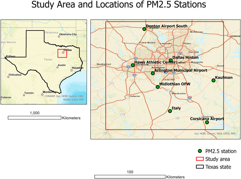
FIGURE 1. Locations of PM2.5 stations in the study area.
2.2 Data
The study used two sets of input data: 1) aerosol optical depth (AOD) and AOD-related variables from MODIS 2) meteorological data to estimate PM2.5 corresponding to the hour of MODIS overpass time.
2.2.1 PM2.5
Terra and Aqua satellites, with an equatorial crossing time of ∼10:30 a.m. and 1:30 p.m. (local time) respectively, overpass the study area twice a day. Nevertheless, due to the broader swath of 2,330 km, MODIS AOD is sometimes available at times other than overpass times. PM2.5 data from ground monitoring stations are available at an hourly interval. The study used PM2.5 for the hour MODIS overpasses the study area. For example, if MODIS overpasses at 10:30 a.m., the PM2.5 measured between 10 a.m. and 11 a.m. was used. The data was downloaded from the Environmental Protection Agency’s website (https://aqs.epa.gov/aqsweb/airdata/download_files.html#Raw) with the parameter code of the PM2.5 data 88502. A total of 10-year PM2.5 observations from 2006–2015 were downloaded for the study area.
2.2.2 AOD data
MODIS AOD data have been available only at 10 km resolution. A recently developed algorithm, Multi-Angle Implementation of Atmospheric Correction (MAIAC) downscales AOD to 1 km resolution (Lyapustin and Wang, 2018). At 10-km resolution, two separate algorithms, Dark Target (DT) and Deep Blue (DB) retrieve aerosols from MODIS data. DT retrieves AOD data for dark/vegetated land surfaces, whereas DB works wells for bright land surfaces. In contrast, MAIAC retrieves aerosols over both dark and bright land surfaces. Besides providing AOD data at a finer spatial resolution, AOD data from MAIAC has better spatial coverage, higher retrieval frequency, low bias, and high correlation with AOD from the Aerosol Robotic Network (AERONET) stations (Superczynski et al., 2017; Jethva et al., 2019; Mhawish et al., 2019).
Because of the superiority of AOD data from MAIAC over other AOD algorithms and its availability at a higher resolution, this study selected the MCD19A2 version-6 data product for AOD estimated with MAIAC algorithm (hereafter, MAIAC AOD data). AOD is available at two wavelengths: 470 nm and 550 nm. This study used AOD at 470 nm because AOD provided at 550 nm is derived from AOD at 470 nm, and AOD at 550 nm is marginally inferior in quality compared to AOD at 470 nm (Lyapustin and Wang, 2018). MAIAC AOD data was transformed to WGS 1984 coordinate system using MODIS Reprojection Tool (MRT), and then space and time references of the MAIAC AOD were used to extract matching PM2.5 observations from the air quality monitoring stations. MAIAC AOD data also provided quality flags for AOD and data on satellite retrieved water vapor content and viewing zenith angle. This study used these variables along with MAIAC AOD. Data about the zenith angle were available at 5 km resolution. Zenith angle data were resampled using nearest neighbor resampling to match the resolution of AOD data.
2.2.3 Meteorological data
Meteorological data came from European Centre for Medium-range Weather Forecast (ECMWF). ECMWF provides reanalysis data worldwide, at 3, 6, 9, and 12 h from 0:00 and 12:00 UTC (Berrisford et al., 2011). Thus, the ECMWF reanalysis data were available for the Dallas-Fort Worth metroplex four times a day, at 9 a.m., 12 p.m., 3 p.m., and 6 p.m. local standard time, and at a spatial resolution of 0.125° (∼13 km). The reanalysis data combine weather observations with the most up-to-date weather models and provide information on different weather variables as a continuous grid at each of the 4 hours (Parker, 2016). The various weather parameters obtained from ECMWF included horizontal and vertical components of the wind, wind gust, temperature, dew point temperature, clear sky surface photosynthetically active radiations, total precipitation, boundary layer height, boundary layer dissipation, total cloud cover, medium cloud cover, high cloud cover, convective precipitation, convective available potential energy, and evaporation. The study retrieved meteorological data closer (in time) to satellite acquisition time.
In total, the study used 21 predictor variables (see Table 1) to model PM2.5 from 8 air quality monitoring stations around the Dallas-Fort Worth area. The first four predictors came from MODIS MAIAC AOD products, and the remaining variables were from ECMWF reanalysis data. Predictors obtained from MODIS data presented instantaneous observations at the time of satellite passing, whereas ECMWF reanalysis data provided four estimates per day.
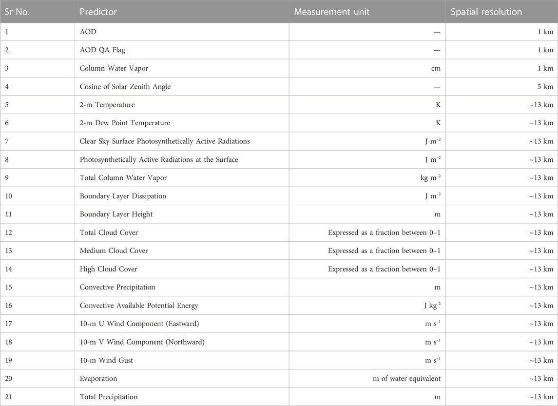
TABLE 1. List of predictors.
2.3 Methodology
Figure 2 shows the flowchart of the data and method used in the study. The study resampled meteorological data to match the resolution of the MAIAC AOD data using the nearest neighbor resampling method. This section discusses data processing, model architecture, and evaluation.
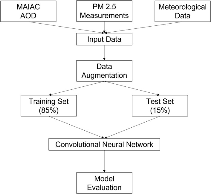
FIGURE 2. Flowchart of data and methodology.
Through convolution operations, the Convolutional Neural Network (CNN) algorithm takes into account the very spatial nature of the images. It applies two-dimensional filters, also known as kernels, on the input. The filter moves over the input image and extracts features. Two-dimensional filters applied to compute convolutional layers use values of spatially adjacent pixels for feature extractions. This process, also known as convolution, exploits the spatial patterns and relationships (Dumoulin and Visin, 2016). An optimization algorithm with backward propagation minimizing a loss function determines weights in these filters (Indolia et al., 2018). These weights define the nature of the spatial relationship among spatially adjacent grid-cells yielding the output (LeCun et al., 1998). For the phenomenon affected by explanatory variables in the surrounding areas, it is essential to account for the influence of spatially adjacent locations. As discussed in the introduction, many studies have improved the performance of models estimating PM2.5 after considering a correlation among variables in space. Specifically, many studies incorporated a weighted average of PM2.5 from nearby stations. Their approach captured existing spatial autocorrelation in the PM2.5 values across in situ stations for PM2.5 estimation even though these stations might be too sparse to acquire PM2.5 spatial variances among them. On the contrary, our study intended to develop a model that relies on variables other than spatially lagged PM2.5 and thus may help explore the effects of other explanatory variables on PM2.5. Therefore, we did not use measurements from nearby PM2.5 monitoring stations but aimed to develop a model that uses AOD and meteorological data to estimate PM2.5 corresponding to an hour of AOD acquisition at specific sites.
Park et al. (2020) investigated spatially lagged variables over a fixed distance using an image size of 5 × 5 but due to the coarser resolution of the AOD data (10 km) they used, it corresponded to an area of 50 km × 50 km. Instead, this study examined the influence of spatial lag size to evaluate the spatial scale effects of meteorological variables with AOD on PM2.5 estimates. The underlying grid resolution of AOD data was 1 km × 1 km. CNN accepts images as input. We located the grid cell in which the particular PM2.5 station is located and expanded upon that grid cell to extract a 3 km × 3 km image. We followed a similar process for all predictor variables- AOD quality flag data, column water vapor, resampled zenith angle, and meteorological data. Since there are 21 predictors, the input image-patch size for one PM2.5 observation from a particular PM2.5 station is 3 × 3 × 21. The process was repeated for all PM2.5 observations from eight monitoring stations in the study area during 2006–2015 to form an input dataset to build a model in an O-CV approach. Similarly, we extracted image-patches of sizes 5 × 5, 7 × 7, 9 × 9, … 19 × 19 to form a total of nine different input datasets (Figure 3). We stopped at 19 × 19 because of the gaps in AOD data due to cloud cover (more discussion in Section 2.3.2). With a PM2.5 station in a central cell, the input image-patch size represented the size of the area around the PM2.5 station. Thus, it was analogous to the concept of spatial lag in spatial statistics. A total of nine CNN models, one for each image-patch size, were developed and compared to evaluate the effect of input image-patch size on PM2.5 estimation.
FIGURE 3. Different sized image-patches centered on a cell with a PM2.5 station.
2.3.1 CNN models of PM2.5 predictions
A larger image contains more information. With larger sizes, spatial relations become more intricate. A neural network learns to recognize more complex features with more convolution layers (Lopez Pinaya et al., 2020). Therefore, depending on the size, the study used variable convolutional layers to account for varying complexity in spatial relations. This led to nine separate CNN models, one for each image-patch size. The larger the image-patch, the more convolutional layers are. Predictors were convoluted using filters of size 3 × 3 until the input image-patch reduces to 1 × 1. The first and the second convolutions consisted of 24 and 16 filters, respectively, whereas each of the remaining convolutions consisted of eight. Each of the dense or fully connected layers had eight neurons. Input image-patches of sizes 3 × 3 and 5 × 5 required only one and two convolutions, respectively, whereas the remaining input image-patch sizes required more than two convolutions. A 7 × 7 image-patch required three convolutions, whereas a 19 × 19 image-patch required seven convolutions. Figure 4 shows the architecture of the CNN used in the study for a 7 × 7 image-patch. A blue square represents 3 × 3 filters used in all convolutions. The study used a sigmoid activation function for all layers except for the last year, which outputs the model predictions with a linear activation function, since the sigmoid limits the output range from 0 to 1 and the linear activation regressed the predictions. The study used the Adam optimization algorithm, an extension to the stochastic gradient decent and appropriate for non-stationary objectives, problems with noisy or sparse gradients, and computationally efficient, and typically low demand on tuning parameters (Kingma and Ba, 2014). The study set a learning rate of 0.01 and 200 epochs for training. The learning rate of 0.01 was found to balance learning time and accuracy. To minimize parameters for training, the study used stride one and no padding across all convolutions. Also, batch normalization followed each convolution and dense layer prior to the ensuing activation function.
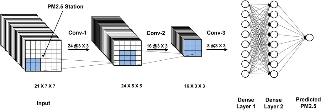
FIGURE 4. The study’s CNN architecture.
2.3.2 Data augmentation
AOD data can be missing due to clouds, snow or brighter surface conditions. The problem of missing data in AOD was well documented in the literature (Goldberg et al., 2019; Hu et al., 2017; Park et al., 2020). The study included only those data points for which AOD data was available for cells in an image-patch of considered size. This problem of missing AOD led to decreasing number of samples for larger image-patch sizes in our study (Table 2). A larger image-patch comprised of more cells than a smaller image-patch, and the chances of having at least 1 cell with missing AOD were greater for larger image-patch sizes. Due to the limited number of samples available for larger image-patch sizes, we restricted our largest input image-patch size to 19 × 19.
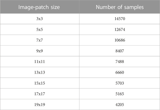
TABLE 2. AOD data availability.
Machine learning approaches, such as CNN, require a large number of samples or data points. The relatively small study area and only 10 years of the study period resulted in small samples in the context of machine learning. Data augmentation, a common practice used in machine learning to increase the sample size, provided a way to generate additional samples. We used the geometric transformations method to augment available data because it was computationally simple and did not introduce new information to original data. Geometric transformation generates additional samples by flipping, scaling, rotating, and cropping original images (Taylor and Nitschke, 2019). The study flipped and rotated an original image-patch (Figure 5) to generate additional image-patches (Figure 6). Flipping generated mirror copies along an axis, whereas rotation arranged original image-patches in different orientations (Figure 6). Image-patches of all the input variables in a particular sample or data point were flipped or rotated in the same way to form a new sample or data point. As a result, the process of data augmentation only repositioned the original sample or data point without making any change to original data values or their inter-relation in spatial configuration. As the study used six different ways to augment the data (Figure 6), each sample was reconfigured in six different ways, resulting in a 6-fold increase in the number of samples available for training and cross-validation.
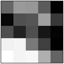
FIGURE 5. Sample image-patch of size 5 × 5.
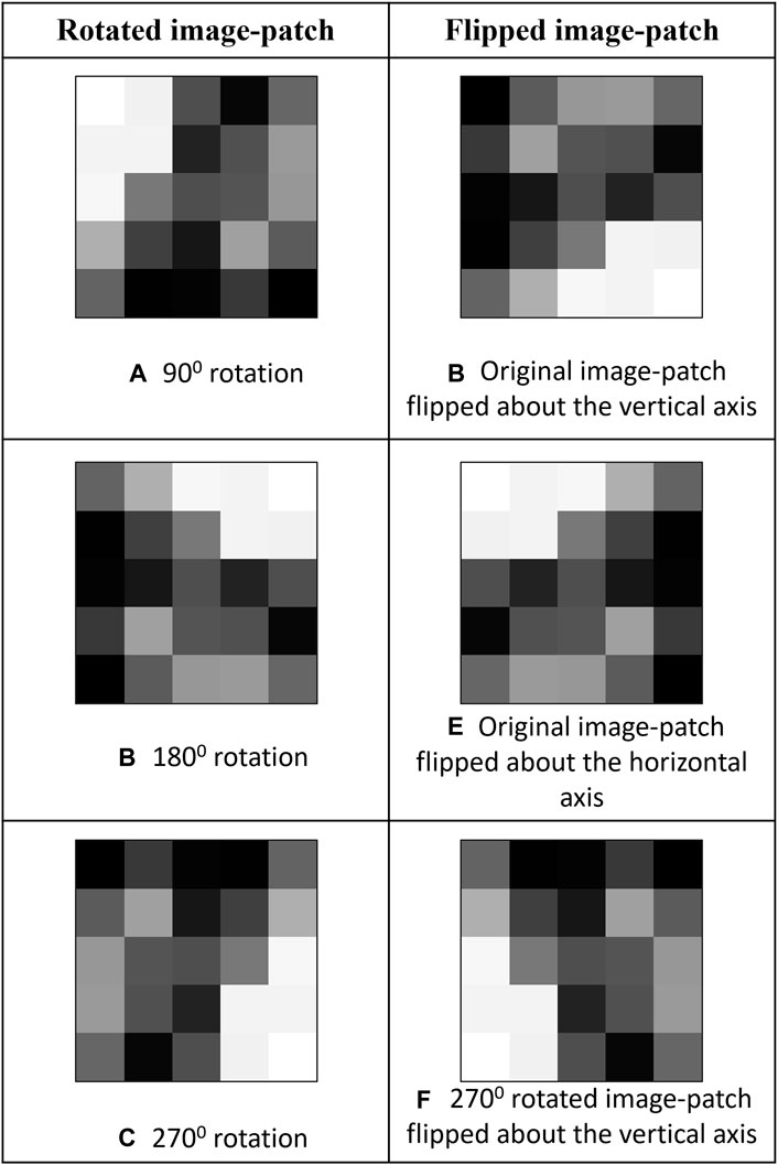
FIGURE 6. Augmented image-patch derived from a sample image-patch in Figure 5.
2.3.3 Cross-validation
As previously noted in the introduction, out of three commonly used cross-validation approaches for AOD-based PM2.5 models, the overall (O-CV) and temporally separated (TS-CV) approaches outperformed the spatially separated approach (SS-CV). The TS-CV approach can result in the training of a model for a specified period. Therefore, this study used the O-CV approach to evaluate model performance. Specifically, the study adopted the five-fold O-CV approach. The data was split into five groups; each group was iteratively used to test the model performance, and the remaining four trained the model. The average correlation coefficient R) and root mean squared error (RMSE) across all five groups were used to compare model performance.
2.3.4 Reliability assessment
The data augmentation technique helped increase the size of the data available for training by generating additional artificial samples from the existing data. However, it raised concerns about the model’s ability to accurately estimate the PM2.5 concentration level of a specific data point regardless of whether it was augmented or not in the training process. In other words, though the same data point was present in the dataset multiple times in different forms, the model’s PM2.5 estimates across these multiple forms may vary. To evaluate the model’s reliability, it was necessary to consider the precision of these estimates or how closely they match each other. We trained a model using an entire dataset (consisting of original data points and augmented data points) and repeated the process for each image-patch size to evaluate the model’s ability to provide precise estimates. The use of the entire dataset for model development enabled the assessment of the variability in PM2.5 estimates of each data point, which we repeated six more times in the augmented dataset. We then calculated the difference between the maximum and minimum estimates (also referred as the range of the PM2.5 estimates) for each data point and calculated the statistics of these values for nine models, each using an input image-patch of a different size.
3 Results
3.1 Description of PM2.5 data
Figure 1 showed the locations of eight monitoring stations in the Dallas-Fort Worth metroplex and its surrounding area. During 2006–2015, the average hourly PM2.5 was 9.29 μg/m3 and 77216 valid hourly PM2.5 measurements were available at satellite image acquisition times across these eight stations (Table 3). The median values at all stations are less than the respective means indicating the positively skewed distribution of PM2.5 concentration at each station. On an average 50% of the values are below 8.29 μg/m3. The average interquartile range of PM2.5 values across all stations is 6.88 μg/m3 with middle 50% values ranging between 5.27 μg/m3 to 12.15 μg/m3. There were several zero and negative values in the data, which were removed based on the assumption that those were the result of potential measurement errors. The table also presents the average hourly PM2.5 level at each station at all available satellite acquisition times during the study period. MODIS acquired data around 10:30 a.m. and 1:30 p.m. The mean PM2.5 value during the satellite acquisition times is lower than the average PM2.5 value at each station because of the improved circulation around noon. PM2.5 values were generally higher in the early morning and late evening.
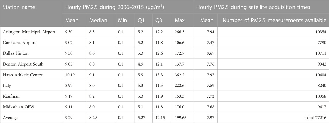
TABLE 3. PM2.5 concentration and data availability during 2006–2015.
AOD data are often susceptible to data gaps due to cloud cover or bright surfaces. The study incurred a high missing rate in AOD data for the same reasons. Image-patches of 3 × 3 km2 with complete AOD data constituted only 18.87% of the total AOD data; those of 19 × 19 km2, merely 5.44%. Table 4 presents the mean and standard deviation of hourly PM2.5 for the different-sized input patches considered in the study. The number of samples (e.g., complete patches) decreased as the patch size increased; the reduced sample size (e.g., number of patches) reduced the mean and standard deviation of PM2.5 available for training the model. PM2.5 decreased from 7.07 μg/m3 to 5.90 μg/m3, and the standard deviation from 5.54 to 4.96 from the smallest to the largest patch size.
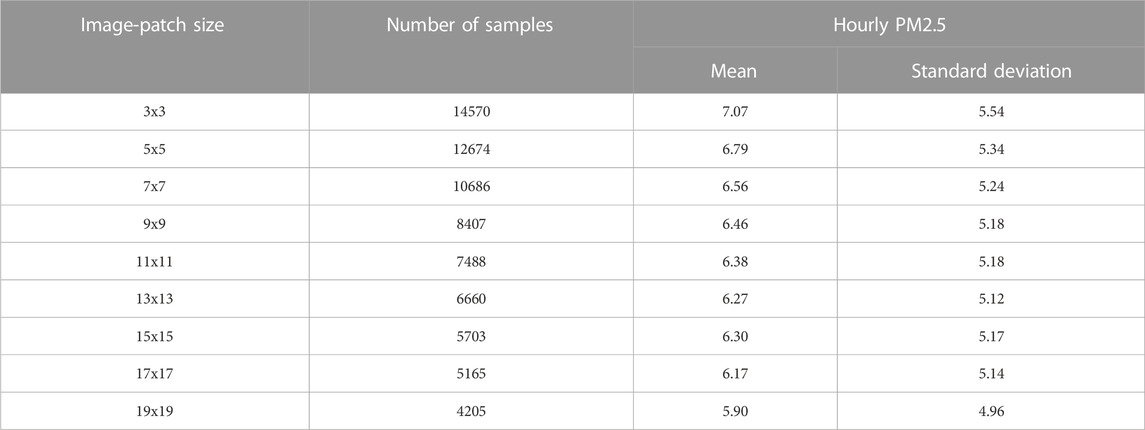
TABLE 4. Descriptive statistics of PM2.5 values across all image sizes.
3.2 Model evaluation
Machine learning methods require a large amount of data to train the model. To overcome the challenge of a limited number of samples to train the model, we used a data augmentation technique to artificially increase the number of samples by introducing relational variance of input data patches to PM2.5 data at the same site and time of MODIS observations. Below are the results of CNN models with augmented data.
Figure 7 shows the results for CNN across different-sized image-patches. Out of all sizes, the model with patch size 19 × 19 km2 performed best with the correlation coefficient R) of 0.87 (or R2 of 0.76) and root mean squared error (RMSE) of 2.57 μg/m3 for PM2.5 estimation at station locations. Unlike other studies in the literature, this study achieved comparably good performance without including PM2.5 covariates from nearby stations. For example, modeling PM2.5 over the contiguous United States, Di et al. (2016) achieved R2 of 0.84, whereas Park et al. (2020) reported R2 of 0.84 and RMSE of 2.55 μg/m3 for 24-h averages of PM2.5. Similarly, a study performed in China for daily PM2.5 estimation reported R2 and RMSE of 0.76 and 13 μg/m3 respectively (Zhan et al., 2017). Because of the differences in the geographic locations and regional extents and levels of air pollution, results from the studies in the literature cannot be directly compared to our results. Noteworthily, our study estimated PM2.5 corresponding to the hour of MODIS data acquisition time in contrast to a 24-h average of PM2.5 in the above-mentioned studies.
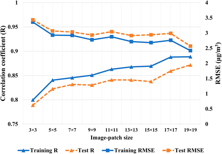
FIGURE 7. Correlation coefficient and RMSE for CNN with varying image-patch sizes with data augmentation.
3.3 Comparison with models not using data augmentation
Without data augmentation, a correlation between estimated PM2.5 from MAIAC AOD and observed PM2.5 at monitoring stations for the training dataset increased with the input image-patch size. However, the correlation degraded for the test dataset (Figure 8). Similarly, the models did not perform as well on the test dataset as the training dataset in terms of RMSE. This suggested that the models performed well on the training dataset with a smaller number of data points but failed to perform equally well over unseen data, a case of overfitting. Finally, we compared the performance of models with and without data augmentation on the test dataset. Data augmentation improved R and decreased RMSE for all image-patch sizes (Figure 9). Moreover, models with larger image-patch sizes, despite relatively small sample size even with data augmentation, outperformed models with smaller-sized image-patches. It suggested that a wider area around the PM2.5 station improved PM2.5 estimation.
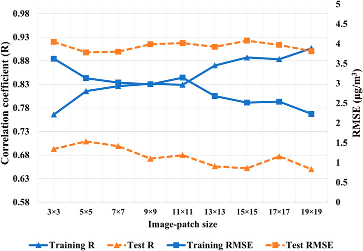
FIGURE 8. Correlation coefficient and RMSE for CNN with varying image-patch size without data augmentation.
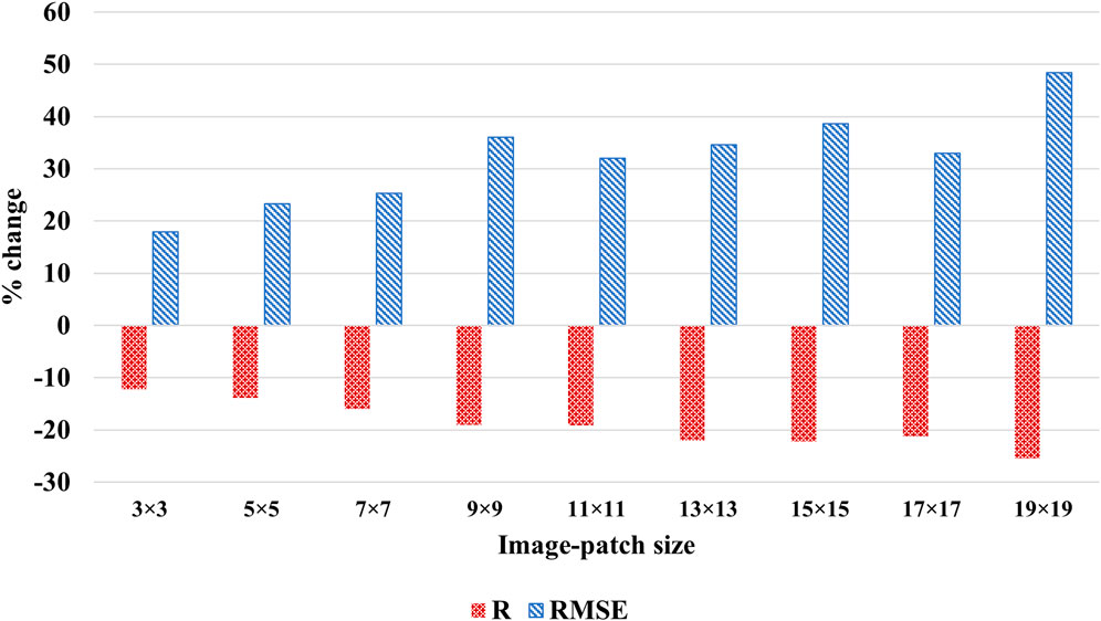
FIGURE 9. Percent change in R and RMSE in models without data augmentation across image-patch sizes.
The implemented data augmentation process retained spatial variance among cells in an input data image-patch (MAIAC AOD and weather data) and the patch’s spatial pattern across all augmented data items but altered the orientation and facing of the patch. No augmentation was applied to in situ observations. Therefore, the data augmentation changed only spatial orientation of the input data associated with a particular observation and, as such, introduced variance to how the interaction between MAIAC-AOD and weather data may relate to in situ PM2.5 observations. The increased relational variance in training data made the model more difficult to converge during the training process (i.e., reaching the set of parameters that minimize the model’s loss function). Meanwhile, the increased variance also lowered the risk of model overfitting. In machine learning, a model is considered overfitting if it performs well on training data but poorly on test data. Figures 7, 8 show the results of CNN models over augmented and non-augmented data, respectively. The R and RMSE values over augmented training and test data are comparable (Figure 7), whereas their apparent discrepancies with non-augmented training and test data suggest poor model performance (Figure 8). As such, the data augmentation helps overcome the data sparsity due to missing AOD without overfitting for PM2.5 estimation in this study.
3.4 Precision evaluation on PM2.5 estimates
The data augmentation technique proved helpful to increase the training data size and improved the model performance. However, due to the repeated data points used in this technique, it was essential to assess the robustness of PM2.5 estimates across these repeated data points. For each image-patch size, a model was developed using the entire dataset to assess the variability in the PM2.5 estimates across the repeated measurements. Table 5 provides descriptive statistics of the difference between maximum and minimum estimates obtained for the same observation across different image-patch sizes. Overall, quartile 1 (Q1), median, and quartile 3 (Q3) values increased as image-patch size increased, while minimum values remained consistently low. However, the magnitude of this increase was relatively small, with the variability only rising from 0.05 for a 3 × 3 image-patch size, 0.58 for 17 × 17, and 0.39 for a 19 × 19 image-patch size. The results suggested that while the precision of the PM2.5 estimates varied across the image-patch sizes, with a smaller patch size producing more precise estimates. Yet, the difference in precision was relatively small. Although the maximum estimated PM2.5 range varied quite a lot across different image-patch sizes, % of values with the range of PM2.5 estimates greater than 2.5 were less than 6.5% across all image-patch sizes, with the lowest percentage of 0.01 for 3 × 3 and the highest percentage of 6.44 for 15 × 15 image-patch size.

TABLE 5. Descriptive statistics of the range of PM2.5 estimates across image-patch sizes.
4 Discussion
In this study, PM2.5 concentration corresponding to the hour of satellite data acquisition time was estimated using the Convolutional Neural Network (CNN) approach for Dallas-Fort Worth metroplex and its surrounding area. A simple CNN model achieved a correlation coefficient of 0.87 and RMSE of 2.57 μg/m3 without using PM2.5 data from nearby monitoring stations (also called spatially lagged PM2.5). In spatial statistics, the spatially lagged dependent variables are used in the model structure to account for the existing spatial dependence in the dependent variable (Anselin, 2003). While these models aim to derive unbiased estimators by accounting for existing spatial autocorrelation in the dependent variable (Anselin and Bera, 1998), for PM2.5 studies, obtaining spatially lagged PM2.5 is challenging because the sparse distribution of air quality monitoring stations may be distant beyond the spatial dependence. Furthermore, PM2.5 come from point (e.g., industry and burns) and non-point (e.g., traffic, diffusion from nearby regions) sources. As such, co-variates from nearby stations may not be useful since a constant spatial gradient between two stations is unlikely. Yet, the convolutional process in our CNN models embedded spatial covariates among MAIAC-AOD cells, which were closer than the distance between nearby stations. In addition, the CNN models also considered spatially lagged independent variables. Without covariates from nearby stations, our best model estimated PM2.5 corresponding to the hour of MODIS data acquisition time, at a finer temporal interval than the 24-h averaged PM2.5 concentration estimated by previous studies.
The MODIS satellite overpasses any area twice a day; however, the recent launch of the geostationary satellite GOES-R has made it possible to acquire AOD data with an increasing frequency of every 5 and 15 min (Schmit et al., 2017). Extending the CNN architecture from this study to these frequently available AOD data will help explore the diurnal trend in PM2.5 and increase the data available for studies investigating the effects of the environmental exposome. In addition, the independent variables used in our model are also readily available everywhere. Therefore, this model can be easily trained for other regions.
This study systematically investigated the effects of the input image-patch size on model performance. The missing AOD problem resulted in a smaller sample size for the larger spatial extents or image-patch sizes considered in the study. The mean and variance of the PM2.5 decreased slightly as the image-patch size increased (Table 4). While it may appear that the improved model performance with larger patch sizes is due to the reduced variance, it is important to note that with a larger spatial extent or patch-size, the model complexity also increased. With larger spatial extents, the model must account for spatial dependence over a larger area around a PM2.5 station. Even with the added complexity and smaller sample size, models with larger image patch-size demonstrated consistently better performance with data augmentation that introduced relational variance in training data. The improved model performance with increased input image-patch size suggests that including spatially lagged independent variables from a wider area around the PM2.5 station improves model performance. Among considered image-patch sizes, image-patch of size 19 km by 19 km performed best with R2 of 0.76 and RMSE of 2.57 μg/m3. With a PM2.5 station at the center, image-patch of size 19 km × 19 km, considers spatially lagged explanatory variables within 10 km of the PM2.5 station. It suggests that adjacent locations as far as 10 km also affect the PM2.5 concentration in addition to local factors, indicating the broader scale at which spatial processes driving PM2.5 are operating. Harrison et al. (2015) collected street-level PM2.5 data in our study region’s 10 km by 10 km area. Their study found that depending on weather conditions, the spatial scale of PM2.5 variation in the area varied between 0.8 and 5.2 km. Thus, depending on the synoptic weather conditions, a smaller image-patch may be sufficient to estimate PM2.5. However, further investigation is required to confirm the same. One way to investigate this is to classify the training dataset into several groups, each group representing homogeneous weather conditions, and investigate if better performance is achieved with a smaller image-patch size in certain conditions.
Although CNN incorporated information from adjacent areas to model PM2.5, this study did not investigate how spatially adjacent locations influence PM2.5 at the estimation location. An explainable AI technique may help uncover this information. Park et al. (2020) used Layerwise Relevance Propagation (LRP) to identify important variables in the model. Their analysis also visualized the spatial pattern of the importance of each predictor. These patterns help investigate how adjacent areas are contributing to PM2.5 concentration. Future studies can use a similar approach to examine the role of adjacent locations, especially in scenarios leading to elevated PM2.5 concentrations. Park et al. (2020) found the weighted average of spatially lagged PM2.5 to be the most important variable. Unlike their study, this study did not use spatially lagged PM2.5. Further analysis of the model using explainable AI techniques may help gain insights into how variables other than spatially lagged PM2.5 contribute to PM2.5 concentration and what information about the factors contributing to PM2.5 this model provides compared to models using nearby PM2.5 measurements. Moreover, the use of spatially lagged PM2.5 assumes that the spatial gradient of PM2.5 between two stations is smooth. However, this cannot always hold true as the different point and non-point sources of PM2.5 between stations may vary. In our study area, the average distance between two PM2.5 stations was 36.26 km with a range from 20.17 km to 58.19 km. The convolution process in the CNN allows embedding MAIAC AOD values from grid cells that are closer than the nearby PM2.5 stations. Additionally, our study aimed to develop a MAIAC AOD-based model to estimate hourly PM2.5 corresponding to the satellite data acquisition times.
The study demonstrated that the data augmentation technique, commonly used in computer vision tasks to increase the sample size, can be used to overcome the problem of limited samples due to missing AOD data. Several studies addressed this problem through a data-filling approach (Hu et al., 2014; Goldberg et al., 2019; Meng et al., 2021). However, depending on the factors responsible for incomplete AOD, missing AOD data can be systematic or non-random. As a result, this introduces bias in the model due to reliance on selective data. The data augmentation technique used in the study does not help address this limitation. In contrast, gap-filling methods can help alleviate this problem to some extent by increasing the AOD availability. Nevertheless, the data augmentation method by increasing sample size helps the model learn complex patterns and relationships. Therefore, even when sufficient data is available for model training, it would be interesting to compare models using augmented data with those that do not and how it affects model performance.
Our study is subject to the following limitations, which also present opportunities for future research. Li and Tartarini (2020) showed the impact of human activities on PM2.5 pollution. Our study assumed that AOD embedded the effect of human activities on PM2.5. However, the AOD is available at 1 km resolution, and human activities can vary widely in 1 km2. Additionally, grid-cells of 1 km spatial resolution are used to obtain point-level PM2.5 measurements from ground monitoring stations. This spatial mismatch can be remedied to some extent by including fine-grained information on human activities associated with PM2.5 pollution such as traffic and other emission sources, especially when human-activity patterns are highly variable over short distances. Another spatial mismatch issue arises because of the position of a PM2.5 station in the assigned grid cell of the input data. Because of the coarser resolution of the input datasets (1 km, 5 km and 13 km), some PM2.5 stations may fall near the center of the cell while others may fall near the edge. One solution to this problem is to resample the data to ensure the PM2.5 station is centrally located in a grid cell. However, resampling is subjected to additional errors and uncertainty in the data. Weather-related variables used in the study had the coarsest resolution of 13 km among all the input variables. However, as weather variables vary at a mesoscale, values between adjacent cells do not vary much. That the model at 19 km × 19 km performed the best also supports that the position of the PM2.5 station with respect to the cell center will not affect the results. Due to insufficient MAIAC-AOD data, the study could not test spatial extents around PM2.5 stations or sensitivity tests beyond 19 × 19 km2. MODIS acquisitions are vulnerable to cloudy conditions that result in data gaps. While statistical methods can interpolate the missing data gaps (Yang and Hu, 2018), our study used only available AOD data to avoid additional uncertainty from interpolated errors. Moreover, PM2.5 estimates showed variability when repeated data points were taken after data augmentation. While this variability was relatively small across different input image-patch sizes, future studies may explore its causes.
Data availability statement
The raw data supporting the conclusions of this article will be made available by the corresponding author, without undue reservation.
Author contributions
MY and YK- conception; YK-design, data collection, analysis, interpretation of results, and original draft preparation, review, and editing; MY-supervision, review, and editing.
Funding
The research was partially supported by funds from the University of Texas System STAR program, the School of Economic, Political, and Policy Sciences at the University of Texas at Dallas, and a scholarship from Pioneer Natural Resources, Inc. The authors declare that this study received funding from Pioneer Natural Resources, Inc. The funder was not involved in the study design, collection, analysis, interpretation of data, the writing of this article, or the decision to submit it for publication.
Conflict of interest
The authors declare that the research was conducted in the absence of any commercial or financial relationships that could be construed as a potential conflict of interest.
Publisher’s note
All claims expressed in this article are solely those of the authors and do not necessarily represent those of their affiliated organizations, or those of the publisher, the editors and the reviewers. Any product that may be evaluated in this article, or claim that may be made by its manufacturer, is not guaranteed or endorsed by the publisher.
References
Anselin, L., and Bera, A. (1998). “Spatial dependence in linear regression models with an introduction to spatial econometrics,” in Handbook of applied economic statistics. Editor A. Ullah (New York: CRC Press), 237–290.
Anselin, L. (2003). “Spatial econometrics,” in A companion to theoretical econometrics (Malden, MA, USA: Blackwell Publishing Ltd), 310–330. doi:10.1002/9780470996249.ch15
Bell, M. L., Dominici, F., Ebisu, K., Zeger, S. L., and Samet, J. M. (2007). Spatial and temporal variation in PM2.5 chemical composition in the United States for health effects studies. Environ. Health Perspect. 115, 989–995. doi:10.1289/ehp.9621
Berrisford, P., Dee, D. P., Poli, P., Brugge, R., Fielding, M., Fuentes, M., et al. (2011). The ERA-Interim archive Version 2.0. 23. Available at: https://www.ecmwf.int/node/8174.
Chen, H., Kwong, J. C., Copes, R., Hystad, P., van Donkelaar, A., Tu, K., et al. (2017). Exposure to ambient air pollution and the incidence of dementia: A population-based cohort study. Environ. Int. 108, 271–277. doi:10.1016/j.envint.2017.08.020
Chudnovsky, A., Lyapustin, A., Wang, Y., Tang, C., Schwartz, J., and Koutrakis, P. (2014). High resolution aerosol data from MODIS satellite for urban air quality studies. Central Eur. J. Geosciences 6, 17–26. doi:10.2478/s13533-012-0145-4
Cohen, A. J., Brauer, M., Burnett, R., Anderson, H. R., Frostad, J., Estep, K., et al. (2017). Estimates and 25-year trends of the global burden of disease attributable to ambient air pollution: An analysis of data from the global burden of diseases study 2015. Lancet 389, 1907–1918. doi:10.1016/S0140-6736(17)30505-6
Di, Q., Kloog, I., Koutrakis, P., Lyapustin, A., Wang, Y., and Schwartz, J. (2016). Assessing PM2.5 exposures with high spatiotemporal resolution across the continental United States. Environ. Sci. Technol. 50, 4712–4721. doi:10.1021/acs.est.5b06121
Dumoulin, V., and Visin, F. (2016). A guide to convolution arithmetic for deep learning. Montreal, Quebec. doi:10.48550/arxiv.1603.07285
Engel-Cox, J. A., Holloman, C. H., Coutant, B. W., and Hoff, R. M. (2004). Qualitative and quantitative evaluation of MODIS satellite sensor data for regional and urban scale air quality. Atmos. Environ. 38, 2495–2509. doi:10.1016/j.atmosenv.2004.01.039
Geng, G., Zhang, Q., Martin, R. v., van Donkelaar, A., Huo, H., Che, H., et al. (2015). Estimating long-term PM2.5 concentrations in China using satellite-based aerosol optical depth and a chemical transport model. Remote Sens. Environ. 166, 262–270. doi:10.1016/J.RSE.2015.05.016
Goldberg, D. L., Gupta, P., Wang, K., Jena, C., Zhang, Y., Lu, Z., et al. (2019). Using gap-filled MAIAC AOD and WRF-Chem to estimate daily PM2.5 concentrations at 1 km resolution in the Eastern United States. Atmos. Environ. 199, 443–452. doi:10.1016/J.ATMOSENV.2018.11.049
Guo, J., Xia, F., Zhang, Y., Liu, H., Li, J., Lou, M., et al. (2017). Impact of diurnal variability and meteorological factors on the PM2.5 - AOD relationship: Implications for PM2.5 remote sensing. Environ. Pollut. 221, 94–104. doi:10.1016/j.envpol.2016.11.043
Gupta, P., and Christopher, S. A. (2009a). Particulate matter air quality assessment using integrated surface, satellite, and meteorological products: 2. A neural network approach. J. Geophys. Res. Atmos. 114, D20205. doi:10.1029/2008JD011497
Gupta, P., and Christopher, S. A. (2009b). Particulate matter air quality assessment using integrated surface, satellite, and meteorological products: Multiple regression approach. J. Geophys. Res. Atmos. 114, 14205. doi:10.1029/2008JD011496
Gupta, P., Doraiswamy, P., Levy, R., Pikelnaya, O., Maibach, J., Feenstra, B., et al. (2018). Impact of California fires on local and regional air quality: The role of a low-cost sensor network and satellite observations. Geohealth 2, 172–181. doi:10.1029/2018gh000136
Harrison, W. A., Lary, D., Nathan, B., and Moore, A. G. (2015). The neighborhood scale variability of airborne particulates. J. Environ. Prot. (Irvine, Calif. 06, 464–476. doi:10.4236/jep.2015.65045
Hu, X., Belle, J. H., Meng, X., Wildani, A., Waller, L. A., Strickland, M. J., et al. (2017). Estimating PM2.5 concentrations in the conterminous United States using the random forest approach. Environ. Sci. Technol. 51, 6936–6944. doi:10.1021/acs.est.7b01210
Hu, X., Waller, L. A., Al-Hamdan, M. Z., Crosson, W. L., Estes, M. G., Estes, S. M., et al. (2013). Estimating ground-level PM2.5 concentrations in the southeastern U.S. using geographically weighted regression. Environ. Res. 121, 1–10. doi:10.1016/J.ENVRES.2012.11.003
Hu, X., Waller, L. A., Lyapustin, A., Wang, Y., Al-Hamdan, M. Z., Crosson, W. L., et al. (2014). Estimating ground-level PM2.5 concentrations in the Southeastern United States using MAIAC AOD retrievals and a two-stage model. Remote Sens. Environ. 140, 220–232. doi:10.1016/j.rse.2013.08.032
Indolia, S., Goswami, A. K., Mishra, S. P., and Asopa, P. (2018). Conceptual understanding of convolutional neural network- A deep learning approach. Procedia Comput. Sci. 132, 679–688. doi:10.1016/J.PROCS.2018.05.069
Jethva, H., Torres, O., and Yoshida, Y. (2019). Accuracy assessment of MODIS land aerosol optical thickness algorithms using AERONET measurements over North America. Atmos. Meas. Tech. 12, 4291–4307. doi:10.5194/AMT-12-4291-2019
Kingma, D. P., and Ba, J. L. (2014). “Adam: A method for stochastic optimization,” in 3rd International Conference on Learning Representations, ICLR 2015 - Conference Track Proceedings, San Diego, California, May 7–9, 2014. doi:10.48550/arxiv.1412.6980
Kioumourtzoglou, M. A., Schwartz, J. D., Weisskopf, M. G., Melly, S. J., Wang, Y., Dominici, F., et al. (2016). Long-term PM2.5 exposure and neurological hospital admissions in the northeastern United States. Environ. Health Perspect. 124, 23–29. doi:10.1289/ehp.1408973
Lary, D. J., Faruque, F. S., Malakar, N., Moore, A., Roscoe, B., Adams, Z. L., et al. (2014). Estimating the global abundance of ground level presence of particulate matter (PM2.5). Geospat Health 8, 611. doi:10.4081/gh.2014.292
LeCun, Y., Bottou, L., Bengio, Y., and Haffner, P. (1998). Gradient-based learning applied to document recognition. Proc. IEEE 86, 2278–2324. doi:10.1109/5.726791
Lee, H. J. (2019). Benefits of high resolution PM 2.5 prediction using satellite MAIAC AOD and land use regression for exposure assessment: California examples. Environ. Sci. Technol. 53, 12774–12783. doi:10.1021/acs.est.9b03799
Li, J., and Tartarini, F. (2020). Changes in air quality during the COVID-19 lockdown in Singapore and associations with human mobility trends. Aerosol Air Qual. Res. 20, 1748–1758. doi:10.4209/AAQR.2020.06.0303
Li, T., Shen, H., Yuan, Q., Zhang, X., and Zhang, L. (2017). Estimating ground-level PM2.5 by fusing satellite and station observations: A geo-intelligent deep learning approach. Geophys Res. Lett. 44 (11), 11,985–11,993. doi:10.1002/2017GL075710
Lopez Pinaya, W. H., Vieira, S., Garcia-Dias, R., and Mechelli, A. (2020). Convolutional neural networks. Mach. Learn. Methods Appl. Brain Disord., 173–191. doi:10.1016/B978-0-12-815739-8.00010-9
Lyapustin, A., and Wang, Y. (2018). MODIS multi-angle implementation of atmospheric correction (MAIAC) data user’s guide collection 6 (ver. Of june 2018) version 2.0. Greenbelt, Maryland.
Meng, X., Liu, C., Zhang, L., Wang, W., Stowell, J., Kan, H., et al. (2021). Estimating PM2.5 concentrations in Northeastern China with full spatiotemporal coverage, 2005–2016. Remote Sens. Environ. 253, 112203. doi:10.1016/J.RSE.2020.112203
Mhawish, A., Banerjee, T., Sorek-Hamer, M., Lyapustin, A., Broday, D. M., and Chatfield, R. (2019). Comparison and evaluation of MODIS multi-angle implementation of atmospheric correction (MAIAC) aerosol product over south asia. Remote Sens. Environ. 224, 12–28. doi:10.1016/J.RSE.2019.01.033
Nam, J., Kim, S. W., Park, R. J., Park, J. S., and Park, S. S. (2018). Changes in column aerosol optical depth and ground-level particulate matter concentration over East Asia. Air Qual. Atmos. Health 11, 49–60. doi:10.1007/s11869-017-0517-5
Özkaynak, H., Baxter, L. K., Dionisio, K. L., and Burke, J. (2013). Air pollution exposure prediction approaches used in air pollution epidemiology studies. J. Expo. Sci. Environ. Epidemiol. 23, 566–572. doi:10.1038/jes.2013.15
Park, Y., Kwon, B., Heo, J., Hu, X., Liu, Y., and Moon, T. (2020). Estimating PM2.5 concentration of the conterminous United States via interpretable convolutional neural networks. Environ. Pollut. 256, 113395. doi:10.1016/j.envpol.2019.113395
Parker, W. S. (2016). Reanalyses and observations: What’s the Difference? Bull. Am. Meteorol. Soc. 97, 1565–1572. doi:10.1175/BAMS-D-14-00226.1
Ramsey, J. B. (1969). Tests for specification errors in classical linear least-squares regression analysis. J. R. Stat. Soc. Ser. B Methodol. 31, 350–371. doi:10.1111/J.2517-6161.1969.TB00796.X
Schmit, T. J., Griffith, P., Gunshor, M. M., Daniels, J. M., Goodman, S. J., and Lebair, W. J. (2017). A closer look at the ABI on the GOES-R Series. Bull. Am. Meteorol. Soc. 98, 681–698. doi:10.1175/BAMS-D-15-00230.1
Stafoggia, M., Schwartz, J., Badaloni, C., Bellander, T., Alessandrini, E., Cattani, G., et al. (2017). Estimation of daily PM10 concentrations in Italy (2006–2012) using finely resolved satellite data, land use variables and meteorology. Environ. Int. 99, 234–244. doi:10.1016/j.envint.2016.11.024
Superczynski, S. D., Kondragunta, S., and Lyapustin, A. I. (2017). Evaluation of the multi-angle implementation of atmospheric correction (MAIAC) aerosol algorithm through intercomparison with VIIRS aerosol products and AERONET. J. Geophys Res. 122, 3005–3022. doi:10.1002/2016JD025720
Taylor, L., and Nitschke, G. (2019). “Improving deep learning with generic data augmentation,” in Proceedings of the 2018 IEEE Symposium Series on Computational Intelligence (SSCI), 1542–1547. doi:10.1109/SSCI.2018.8628742
Tian, J., and Chen, D. (2010). A semi-empirical model for predicting hourly ground-level fine particulate matter (PM2.5) concentration in southern Ontario from satellite remote sensing and ground-based meteorological measurements. Remote Sens. Environ. 114, 221–229. doi:10.1016/j.rse.2009.09.011
U.S. Environmental Protection Agency (2017). National emissions inventory: January 2021 updated release, technical support document. Available at: https://www.epa.gov/sites/default/files/2021-02/documents/nei2017_tsd_full_jan2021.pdf (Accessed March 31, 2022).
van Donkelaar, A., Martin, R. v., Spurr, R. J. D., and Burnett, R. T. (2015). High-resolution satellite-derived PM2.5 from optimal estimation and geographically weighted regression over north America. Environ. Sci. Technol. 49, 10482–10491. doi:10.1021/ACS.EST.5B02076/ASSET/IMAGES/MEDIUM/ES-2015-02076K_0008.GIF
Xie, Y., Wang, Y., Zhang, K., Dong, W., Lv, B., and Bai, Y. (2015). Daily estimation of ground-level PM2.5 concentrations over beijing using 3 km resolution MODIS AOD. Environ. Sci. Technol. 49, 12280–12288. doi:10.1021/acs.est.5b01413
Xu, J., Jiang, H., Zhang, X., Lu, X., and Peng, W. (2014). Study on spatial-temporal variation of aerosol optical depth over the Yangtze Delta and the impact of land-use/cover. Int. J. Remote Sens. 35, 1741–1755. doi:10.1080/01431161.2014.882033
Yang, J., and Hu, M. (2018). Filling the missing data gaps of daily MODIS AOD using spatiotemporal interpolation. Sci. Total Environ. 633, 677–683. doi:10.1016/J.SCITOTENV.2018.03.202
Zhan, Y., Luo, Y., Deng, X., Chen, H., Grieneisen, M. L., Shen, X., et al. (2017). Spatiotemporal prediction of continuous daily PM2.5 concentrations across China using a spatially explicit machine learning algorithm. Atmos. Environ. 155, 129–139. doi:10.1016/j.atmosenv.2017.02.023
Keywords: PM2.5, MODIS MAIAC, aerosol optic depth, convolational neural netwwork, spatial lag effect
Citation: Karale Y and Yuan M (2023) Spatially lagged predictors from a wider area improve PM2.5 estimation at a finer temporal interval—A case study of Dallas-Fort Worth, United States. Front. Remote Sens. 4:1041466. doi: 10.3389/frsen.2023.1041466
Received: 10 September 2022; Accepted: 23 January 2023;
Published: 13 February 2023.
Edited by:
Hannah Victoria Herrero, The University of Tennessee, United StatesReviewed by:
Joseph P. Messina, University of Alabama, United StatesErin Bunting, Michigan State University, United States
Copyright © 2023 Karale and Yuan. This is an open-access article distributed under the terms of the Creative Commons Attribution License (CC BY). The use, distribution or reproduction in other forums is permitted, provided the original author(s) and the copyright owner(s) are credited and that the original publication in this journal is cited, in accordance with accepted academic practice. No use, distribution or reproduction is permitted which does not comply with these terms.
*Correspondence: Yogita Karale, a2FyYWxlLjFAb3N1LmVkdSYjeDAyMDBhOw==