 Zhipeng Tang
 Hari Adhikari
 Petri K. E. Pellikka
 Janne Heiskanen
- 1Department of Geosciences and Geography, Faculty of Science, University of Helsinki, Helsinki, Finland
- 2Institute for Atmospheric and Earth System Research, Faculty of Science, University of Helsinki, Helsinki, Finland
- 3AFRY Management Consulting Oy, Vantaa, Finland
Preprocessing of Landsat images is a double-edged sword, transforming the raw data into a useful format but potentially introducing unwanted values with unnecessary steps. Through recovering missing data of satellite images in time series analysis, gap-filling is an important, highly developed, preprocessing procedure, but its necessity and effects in numerous Landsat applications, such as tree canopy cover (TCC) modelling, are rarely examined. We address this barrier by providing a quantitative comparison of TCC modelling using predictor variables derived from Landsat time series that included gap-filling versus those that did not include gap-filling and evaluating the effects that gap-filling has on modelling TCC. With 1-year Landsat time series from a tropical region located in Taita Hills, Kenya, and a reference TCC map in 0–100 scales derived from airborne laser scanning data, we designed comparable random forest modelling experiments to address the following questions: 1) Does gap-filling improve TCC modelling based on time series predictor variables including the seasonal composites (SC), spectral-temporal metrics (STMs), and harmonic regression (HR) coefficients? 2) What is the difference in TCC modelling between using gap-filled pixels and using valid (actual or cloud-free) pixels? Two gap-filling methods, one temporal-based method (Steffen spline interpolation) and one hybrid method (MOPSTM) have been examined. We show that gap-filled predictors derived from the Landsat time series delivered better performance on average than non-gap-filled predictors with the average of median RMSE values for Steffen-filled and MOPSTM-filled SC’s being 17.09 and 16.57 respectively, while for non-gap-filled predictors, it was 17.21. MOPSTM-filled SC is 3.7% better than non-gap-filled SC on RMSE, and Steffen-filled SC is 0.7% better than non-gap-filled SC on RMSE. The positive effects of gap-filling may be reduced when there are sufficient high-quality valid observations to generate a seasonal composite. The single-date experiment suggests that gap-filled data (e.g. RMSE of 16.99, 17.71, 16.24, and 17.85 with 100% gap-filled pixels as training and test datasets for four seasons) may deliver no worse performance than valid data (e.g. RMSE of 15.46, 17.07, 16.31, and 18.14 with 100% valid pixels as training and test datasets for four seasons). Thus, we conclude that gap-filling has a positive effect on the accuracy of TCC modelling, which justifies its inclusion in image preprocessing workflows.
1 Introduction
Image preprocessing is an important step in remote sensing, typically including operations such as solar angle normalization, atmospheric correction, and topographic correction. Although certain preprocessing procedures are frequently used, there are no “standard” preprocessing steps because the need for preprocessing depends on the specific application and may be determined by personal preference (Campbell and Wynne, 2011). The users of remote sensing data often find making decisions for an appropriate preprocessing workflow challenging because unnecessary steps may create unwanted artifacts, and hence do not necessarily improve the end results of the analysis. Young et al. (2017) proposed a guide and a decision tree to help decide an appropriate level of image preprocessing for common ecological applications. They recommend a parsimonious approach to preprocessing that avoids unnecessary steps and recommend preprocessing steps that are well tested, easily available, and sufficiently documented. Although some of the most common preprocessing steps such as geographic correction and atmospheric correction have been examined, the necessity and effectiveness of gap-filling in remote sensing applications is rarely evaluated. It can be assumed that gap-filling can automatically improve accuracy of the analyses, but it can also be “unnecessary” or even decrease accuracy as gap-filled values are not real radiometric observations. Therefore, it is necessary to study the impact of gap-filling from the application perspective.
The popularity of gap-filling has been rising due to the frequent use of medium spatial resolution data such as Landsat in time series approaches. The advantage of gap-filling is that it handles missing observations (i.e. gaps) caused by clouds, cloud shadows, and sensor failures and can produce images that are visually similar to the originals through learning or interpolating. To date, many gap-filling methods have been proposed, and are categorized into several types (e.g. spatial-based, temporal-based, and hybrid methods), among which, the temporal-based methods have been investigated by the most researchers (Shen et al., 2015). Temporal spline methods, such as Steffen spline interpolation, a 1-dimensional monotonic interpolation based on piecewise cubic functions (Steffen, 1990), has obtained good performance in several studies (Inglada et al., 2015; Hamrouni et al., 2021). Hybrid gap-filling methods have been recently developed in a growing number, among which, Missing Observation Prediction based on Spectral-Temporal Metrics (MOPSTM) has delivered good performance in a short-term time series (Tang et al., 2021). MOPSTM predicts gaps based on valid pixels in the image to be reconstructed and statistical spectral-temporal metrics computed for a 1-year period as feature space using a k-Nearest Neighbor (k-NN) machine-learning method (Tang et al., 2021).
TCC modelling based on remote sensing data, an essential measurement in forest management, vegetation growth cycle monitoring, and disease prevention, has received strong interest in research on mountainous tropical areas (Wang et al., 2005; Anchang et al., 2020; Tang et al., 2020). Measurement of TCC using wall-to-wall airborne lidar is comparable to that using field data (Korhonen et al., 2011) but can provide a large size of samples and enables random samples to be used in inaccessible terrain (Adhikari et al., 2016). However, sensor-based TCC modelling relies heavily on the quality of satellite images that require valid observations in a successive time series (Baccini et al., 2008; Margono et al., 2012), which makes cloud-free satellite images greatly preferred in existing TCC modelling studies (Yang et al., 2012; Karlson et al., 2015; Derwin et al., 2020). The abandonment of incomplete images, in turn, shrinks the amount of data available for TCC modelling in tropical regions, where continuous cloudy weather occurs during rainy seasons (Anderson et al., 2010).
Gap-filling has potential to improve the quality of time series metrics (or composites) that are related to TCC modelling. One popular example is to use image composites, typically referring to cloud-free median reflectance of spectral bands, e.g. the red and near infrared (NIR) bands, or vegetation indices (VIs), e.g. Normalized Difference Vegetation Index (NDVI) (Tucker, 1979) and Enhanced Vegetation Index (EVI) (Liu and Huete, 1995). Seasonal composite (SC) refers to a composite image computed for a particular season, such as rainy and dry seasons in the tropics. SCs characterizing the intra-annual dynamics of vegetation have demonstrated their advantages for several applications (Karlson et al., 2015; Liu et al., 2016; Chaparro et al., 2018). For example, Kushal et al., 2021 developed a spatial and temporal inventory for crop covers using two SCs derived from the Landsat time series. Furthermore, a combination of multiple SCs showed superiority over a single SC when mapping fractional woody cover in semi-arid savannas in South Africa (Higginbottom et al., 2018).
Spectral-temporal metrics (STMs) (Adhikari et al., 2016; Azzari and Lobell, 2017) that reduce the pixelwise spectral variance into statistical metrics such as mean, median, and percentile points, are other widely used tools to derive reflectance and VI metrics for TCC modelling. Examples of the applications that include STMs are pan-European land cover mapping (Pflugmacher et al., 2019), urban-rural gradients of settlements and vegetation mapping (Schug et al., 2020), and global forest canopy height mapping (Potapov et al., 2020).
In addition to SCs and STMs, Fourier (harmonic) analysis has long been used to assess vegetation dynamics and classify basic vegetation formations (Moody and Johnson, 2001; Wang et al., 2019), and delivers good performance in characterizing land surface phenology (Moody and Johnson, 2001). Harmonic regression (HR) coefficients were found to be better predictors for TCC modelling than median composites in Derwin et al. (2020) and Wilson et al. (2018). These two studies, however, did not examine the sensitivity of HR coefficients concerning gaps, as the former used almost cloud-free Landsat images, and the latter pointed out that HR associated with TCC modelling provides a means for overcoming gaps in Landsat time series but lacked a sensitive test for the gaps.
Apart from time series approaches, using a single-date image remains an established approach for applications such as land cover classification (Langley et al., 2001), forest cover change detection (Mayes et al., 2015), and modelling tropical forest canopy height (Ota et al., 2014), tree canopy cover, and aboveground biomass (Karlson et al., 2015). Images in a time series have demonstrated advantages over single-date images (Karlson et al., 2015; Chrysafis et al., 2019), but such approaches are limited by the availability of cloud-free images (Vogeler et al., 2018). When cloud-free images are rarely available, gap-filling can enable the use of partly cloud-covered single-date images.
In this study, our objective was to examine whether gap-filling preprocessing is necessary for TCC modelling and how gap-filling benefits TCC modelling based on annual Landsat time series. We mainly examined our gap-filling method, MOPSTM, which is a hybrid method as it is simple to tune and accurate in reconstructing large-area gaps and continuous time series (Tang et al., 2021). To explore how the selection of gap-filling method affects TCC modelling results, we included a popular temporal-based method, Steffen spline interpolation, for comparison. We selected Steffen spline interpolation because it demonstrated the best performance among several temporal interpolation methods in Tang et al. (2022). The study area encompassed a large Afromontane landscape in Taita Hills, Kenya with seasonally persistent cloud cover and a bimodal rainfall pattern, which poses a challenge for acquiring cloud-free images and applying time series approaches. To evaluate the results quantitatively, a TCC map derived from the airborne laser scanning (ALS) data was used as reference data. This study is organized as follows: 1) We compared the TCC modelling performance based on time series predictors including SCs, STMs, and HR coefficients derived from images that were non-gapfilled and that were gap-filled using Steffen spline and MOPSTM; 2) We used various proportions of MOPSTM gap-filled and valid pixels from single-date images to evaluate how gap-filled pixels deviated from the valid pixels in terms of TCC modelling accuracy.
2 Material and Methods
The workflow of this study is illustrated in Figure 1. The first step was to preprocess the Landsat time series. Then, Landsat time series were used to compute VIs. The two main procedures contained 1) time-series predictor variable experiments to compare TCC modelling performance using Landsat time series that were gap-filled and not gap-filled and 2) single-date predictor variable experiments to compare how gap-filled data deviated from the valid data in TCC modelling.

FIGURE 1. Flowchart of the tree canopy cover modelling experiments using bootstrap sampling random forest regression. Abbreviations: SCs: seasonal composites; STMs, spectral-temporal metrics; HR, harmonic regression.
2.1 Study Area
The study area is located in the Taita Hills (3°18′S, 38°30′E) in southeastern Kenya (Figure 2). The area has variable topography, in which the altitude of hills ranges from around 1,000 to 2,200 m. The surrounding plains have an approximate altitude of between 430 and 1,000 m. This area has a bimodal rainfall pattern—long rains between March and May and short rains between October and December (Pellikka et al., 2009; Pellikka et al., 2013). The main land cover types in this area include bushland, cropland, montane and plantation forests, grassland, and built-up areas (Pellikka et al., 2018).
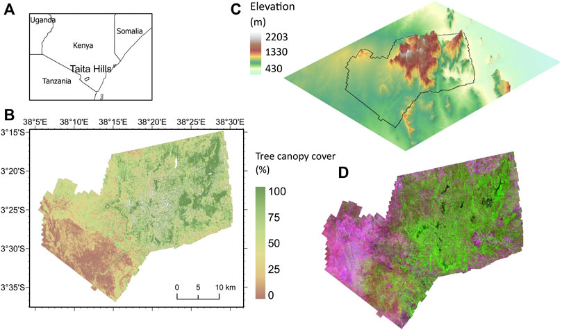
FIGURE 2. Location of the study area with a map of tree canopy cover. (A) The area of interest (Taita Hills) located in Kenya; (B) Tree canopy cover map from the Airborne Laser Scanning data in Taita Hills; (C) 30 m digital surface model (DSM) from the Japan Aerospace Exploration Agency (JAXA) in Taita Hills and (D) An example of Landsat 8 image acquired on 16 December 2015, displayed in R: SWIR1, G: NIR, B: red band.
2.2 Airborne Laser Scanning Data
Airborne Laser Scanning (ALS) data were collected between January 2014 and February 2015 with a Leica ALS60 sensor, pulse rate of 58 kHz, scan rate of 66 Hz, scan angle of ±16°, mean range of 1,460 m, mean pulse density of 3.1 pulses m−2, and mean return density of 3.4 returns m−2. The data were processed into a 2 m resolution digital elevation model, which were used to normalize ALS point cloud elevations to the height above ground level and to remove the returns of noise using LAStools software, rapidlasso GmbH (Adhikari et al., 2016; Heiskanen et al., 2019). The electric lines were removed by manual editing. Finally, reference TCC was calculated at 30 m resolution as a ratio of the first returns from the canopy and the total number of first returns. A 3 m height threshold was used to separate understory and ground returns from the tree canopy returns.
2.3 Landsat Time Series
Landsat 8 Operational Land Imager (OLI) Collection 1 Level-2 Surface Reflectance products for 2015 (Table 1) were obtained from the USGS website1. Pixels contaminated by clouds and cloud shadows were masked out using Fmask (Zhu and Woodcock, 2012). Even so, contaminated pixels were still present in the images. To eliminate the effects of the remaining contaminated pixels (Zhu and Woodcock, 2014), we used only 11 images that have over 70% valid pixels (Derwin et al., 2020). The ultra-blue band that is useful for coastal and aerosol studies (Acharya and Yang, 2015) was eliminated, with reference to other canopy cover studies (Korhonen et al., 2017; Derwin et al., 2020).

TABLE 1. Characteristics of Landsat 8 Operational Land Imager (OLI) images.
As the topographic normalization showed an improvement in the prediction of vegetation biophysical variables in an earlier study (Adhikari et al., 2016), we applied a C-correction method (Teillet et al., 1982) to the six spectral bands (blue, green, red, NIR, SWIR1, and SWIR2) of the Landsat time series. As recommended by Adhikari et al. (2016), Shuttle Radar Topography Mission (SRTM) DEM was used for topographic normalization.
2.4 Gap-Filling Algorithm
We used the Steffen spline method from the open-source software Processing Kernel for geospatial data (Pktools) (Mclnerney and Kempeneers, 2014; Kempeneers, 2018), written in C++ and relying on the GDAL API. It guarantees the monotonicity of the interpolating function between the valid observations in the time series.
To perform MOPSTM, STMs were first derived from the Landsat time series. Then, a k-NN regression model was trained based on the valid pixels in the image to be gap-filled. The last step was to predict the missing observations using the trained k-NN model and STMs. Since our images were acquired in 2015, there was no need to set any temporal window to guarantee a 1-year period when applying MOPSTM.
2.5 Time-Series Predictor Variables
Three time series predictor variables—SCs, STMs, and HR coefficients—were derived from six Landsat 8 spectral bands and five commonly used VIs (Table 2) including EVI, Green Normalized Difference Vegetation Index (GNDVI), Normalized Difference Moisture Index (NDMI), NDVI, and Non-Photosynthetic Vegetation Normalized Difference (NPVND).
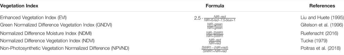
TABLE 2. Summary of vegetation indices using blue, green, red, near infrared, and shortwave infrared spectral bands of Landsat 8 sensors.
2.5.1 Seasonal Composites
Since the study area has a bimodal rainfall pattern, we labelled the four seasons as S1 (dry and hot season, January–February), S2 (long rains, March–May), S3 (dry and cool season, June–September), and S4 (short rains, October–December). Median composites derived for the S1–S4 are labelled as SC1–SC4 (Table 3).
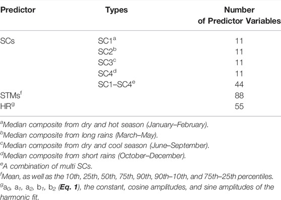
TABLE 3. Model-specific predictor variables. Each predictor includes six spectral bands (blue, green, red, NIR, SWIR1, and SWIR2) and five vegetation indices (EVI, GNDVI, NDMI, NDVI, and NPVND). Abbreviations: SCs: seasonal composites; STMs, spectral-temporal metrics; HR, harmonic regression.
2.5.2 Spectral-Temporal Metrics
Many descriptive metrics can be used to calculate STMs from the time series. Based on the good performance in the previous studies (Potapov et al., 2017; Souverijns et al., 2020), we calculated the mean, as well as the 10th, 25th, 50th, 75th, 90th, 90th–10th, and 75th–25th percentiles of the spectral bands and VIs (Table 3).
2.5.3 Harmonic Regression Coefficients
Considering the bimodal rainfall pattern over a year in our study area, we selected the 2-term harmonic model in Eq. 1 for harmonic regression. The harmonic model formula is, therefore:
where
For convenience, we take SWIR1 data as an example to explain the steps of the experiment. First, we filled the gaps in a SWIR1 band using MOPSTM. Then, both original and gap-filled data were combined into time-series stacks, with each pixel representing a vector of reflectance values chronologically ordered through time. The next step was to calculate the HR coefficients with a harmonic curve fitted to each pixel of the SWIR1 original and gap-filled stacks. Applied successfully in the study of Derwin et al. (2020), the EWMACD algorithm (Brooks, 2014; Brooks et al., 2014) was used to derive five coefficients including the constant, first sine, first cosine, second sine, and second cosine for each pixel. The same experimental procedure was applied to all spectral bands and VIs. The five HR coefficients (Table 3) were subsequently used as predictor variables in the random forest regression (Section 2.7).
2.5.4 Time-Series Experiments
We designed seven experiments to evaluate the effect of gap-filling on the three sets of predictors including SCs, STMs, and HR. To be specific, each experiment contains the same set of predictors, but derived from images that were not gap-filled (actual images) and images that were gap-filled by the Steffen spline and MOPSTM methods. The seven experiments vary based on the combination of predictors used: 1) SC1, 2) SC2, 3) SC3, 4) SC4, 5) a combination of SCs, 6) STMs, and 7) HR.
2.6 Single-Date Predictor Variables
2.6.1 Filling Simulated Gaps in Single-Date Images
To study how gap-filled observations differed from valid observations in terms of modelling accuracy, we selected one image from each season. The four images were acquired from the day of year (DOY) 30, 142, 222, and 350 in 2015 and had as many valid observations as possible during each season. Then, we simulated artificial gaps by removing all the pixels in the four single-date images where the simulated gap rates are 94%, 68%, 56%, and 52%, respectively. The simulated gap rate was not 100% because of the existence of real gaps in these images. We then filled the gaps with pixels from an extension of the study area using MOPSTM (Tang et al., 2021). Because the comparison was between gap-filled and actual pixels, we used the more accurate MOPSTM-gap-filled results (gap-filling performance comparisons of MOPSTM and Steffen spline can be seen in Tang et al. (2022)).
2.6.2 Single-Date Experiments
With the MOPSTM gap-filled and actual images, we designed the experiments to compare their performance in TCC modelling. We selected 10,000 training and test pixels randomly from the overall TCC pixels where the training and test data had no overlaps. The training data were split into a set of proportions of gap-filled and valid pixels from 0, 0.1, 0.2, … , 1, and so were the test data. Then, various combinations of training and test data were used to model and predict TCC. Specifically, for example, the model trained with 0.3/0.7 gap-filled/valid training data was used to predict the test data with 0/1, 0.1/0.9, 0.2/0.8, … , 1 gap-filled/valid test data. We repeated the above steps 100 times to get an average of the accuracy.
2.7 Random Forest Regression
Random forest (RF) method (Ho, 1995) has become popular in modelling vegetation attributes (Vauhkonen et al., 2010; Shataee et al., 2012; Heiskanen et al., 2017) because it has many advantages, such as easy parameter tuning, insensitivity to multicollinearity of the predictor variables and variable selection, and advantages in modelling complex relationships (Ho, 1995; Ali et al., 2012). Therefore, we applied RF to model the relationship between the TCC reference data and predictor variables. We used the “randomForest” package (Liaw and Wiener, 2002) in R environment (Team, 2018). Bootstrap sampling with replacement was applied to evaluate model predictions (James et al., 2013). For each time-series predictor, there were 100 bootstrap samples in which each bootstrap sample contained 10,000 random training pixels and 8,000 random test pixels.
2.8 Accuracy Assessment and Variable Importance
Model accuracy was assessed based on the test data using root mean square error (RMSE) and R2.
where Vi is the ith observed value in the total observations of n,
Variable importance, provided in RF models, is used to measure the importance of the predictor variables by a means of statistical inference. The most advanced variable importance measurement in RF is the “permutation accuracy importance” (Strobl et al., 2007), which compares the difference in accuracy between the original predictor variable and the permuted predictor variable. The measurement is available in the “randomForest” package (Liaw and Wiener, 2002) in R.
To compare the relative importance between the same predictor variables derived from gap-filled or non-gap-filled images, we applied the variable importance method to three types of combinations from SCs, STMs, and HR models that contain both gap-filled and non-gap-filled variables. For the SCs model, we combined SCs from all seasons to demonstrate the variable importance.
3 Results
3.1 Comparisons of Time Series Experiments
3.1.1 Model Accuracy Between Predictors
The non-gap-filled and MOPSTM-gap-filled Landsat reflectance and VIs for DOY 14 in 2015 are illustrated in Figure 3, where MOPSTM produced smooth and natural-looking reconstructed images.
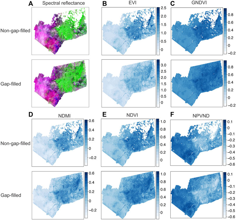
FIGURE 3. The non-gap-filled and MOPSTM-gap-filled images and for the Landsat image acquired on DOY 14 2015. (A) Spectral reflectance displayed in false color of R: SWIR1, G: NIR, and B: red surface reflectance, (B) EVI, (C) GNDVI, (D) DNMI, (E) NDVI, and (F) NPVND. Abbreviations: EVI, enhanced vegetation index; GNDVI, green normalized differential vegetation index; NDMI, normalized difference moisture index; NDVI, normalized difference vegetation index; NPVND, non-photosynthetic vegetation normalized difference.
Figure 4 demonstrates the RMSE and R2 distributions of TCC modelling using SCs, STMs, and HR predictor variables. On average, predictors based on gap-filled images performed better than those without gap-filling. Steffen spline delivered slightly worse accuracy than non-gap-filled data for S1, S3, and STMs, but it surpassed them more greatly for other predictors. MOPSTM indicated better performance than non-gap-filling models for the predictor variables all the predictors, except for SC1. Also, MOPSTM gap-filled SCs showed the greatest improvement in S4 when the median RMSE decreased by approximately 1.8 and the median R2 increased by approximately 0.06.
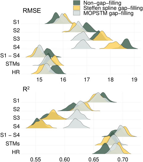
FIGURE 4. Bootstrapping results for the variables using non-gap-filling versus using gap-filling (Steffen spline and MOPSTM methods), predicting the tree canopy cover. The kernel densities are based on 100 bootstrap samples for the tested Landsat reflectance and vegetation indices. A wide spread in kernel density indicates variation among the bootstrap samples. Abbreviations: S1 denotes dry and hot season (January–February), S2 denotes long rains (March–May), S3 denotes dry and cool season (June–September), S4 denotes short rains (October–December), S1–S4 is a combination of all the seasons.
As the number of valid observations of pixels throughout the year can be a driver behind overall RMSE, we examined how the RMSE of SC1–SC4 relies on the number of valid observations used for computing median (Figure 5). When the valid observation was zero in Figures 5D–G, it meant there was no valid data in the specific season, but gap-filling methods can still work based on data from other seasons. However, if there were no valid observations throughout the four seasons, neither Steffen spline nor MOPSTM can work.
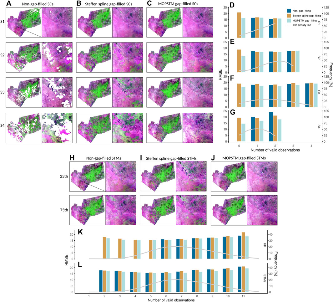
FIGURE 5. Dependence of RMSE on the number of observations for four SCs, STMs and HR coefficients derived from Landsat images that were not gap-filled and images that were gap-filled. (A) SCs without gap-filling; (B) SCs with Steffen spline gap-filling; (C) SCs with MOPSTM gap-filling; (D) SC1 RMSE; (E) SC2 RMSE; (F) SC3 RMSE; (G) SC4 RMSE; (H) STMs (25th and 75th percentile metrics) without gap-filling; (I) STMs (25th and 75th percentile metrics) with Steffen spline gap-filling (J) STMs (25th and 75th percentile metrics) with MOPSTM gap-filling (K) HR RMSE; and (L) STMs RMSE. The x-axis for (D–G), (K,L) is the number of the valid observations of each pixel through the time series, y-axis on the left is the RMSE, y-axis on the right is the frequency (in percentage) of number of valid observations, displayed in grey lines.
A clear improvement after applying MOPSTM gap-filling was observed in all classes of valid observations in SC2–SC4, and the greatest improvement was observed in SC4. For SC1, no improvement after gap-filling was observed when the number of valid observations was 1 or 2, but the MOPSTM RMSE of the zero valid observations case was not worse than when there was at least 1 valid observation. For other seasons, MOPSTM gap-filled results yielded higher accuracy than non-gap-filled results, especially for SC4. Although Steffen spline method had poorer performance than MOPSTM in most SCs, it had higher accuracy than non-gap-filled results for all the cases in SC2 and SC4. Steffen spline method yielded lower accuracy than non-gap-filled results in SC3, one reason for which was that Steffen spline method produced artifacts in SC3 (Figure 5B).
For STMs, RMSE for one valid observations was not shown because Steffen spline did not interpolate values in that case. The largest difference between the non-gap-filled and MOPSTM gap-filled predictors is situated in the 8–11 valid observations through the time series (Figures 5H,J,L). Steffen gap-filling models performed less accurate than non-gap-filling models (Figure 4) because it produced less accurate STMs (Figure 5I).
For the HR model, RMSE is shown for pixels that have six and more than six valid observations (Figure 5K). A clear improvement in MOPSTM gap-filled models depending on the number of observations can be observed in the HR model no matter how many numbers of observations there are through the time series. Steffen spline models had similar results to the non-gap-filling models but was less accurate when the valid number was the largest.
Although the overall RMSE and RMSE stratified by the number of valid observations indicated higher accuracy for MOPSTM gap-filling models than non-gap-filling models, we compared their performance using an additional accuracy measurement, absolute residuals (i.e., the differences between observed and fitted values) in Figure 6. Similar to the results in Figure 5, a greater improvement for MOPSTM gap-filled models was observed when valid numbers were 1, or larger than 7. Minor improvement for MOPSTM gap-filled models, however, can also be found when 2–6 valid observations existed.

FIGURE 6. Dependence of absolute residuals on the number of observations for spectral-temporal metrics (STMs). The x-axis is the number of the valid observations of any one pixel through the time series, and y-axis is the absolute residuals. The gap-filling method was MOPSTM.
3.1.2 Harmonic Curves of Single-Pixel NDVI Time Series
In this section, we show the illustrative harmonic curves of NDVI time series in Figure 7, where the harmonic curves were fitted by only valid pixels and a mix of gap-filled and valid pixels, respectively, across three land cover types—bushland, forest, and cropland. Six pixel locations (Figure 7G) with two bushland types located in (3°27′17.9″S, 38°6′17.2″E) and (3°24′27.0″S, 38°28′53.6″E), two forest types located in (3°18′34.2″S, 38°28′7.1″E) and (3°21′38.7″S, 38°22′5.3″E) and two cropland types located in (3°24′49.2″S, 38°21′50.7″E) and (3°24′17.1″S, 38°26′32.6″E).
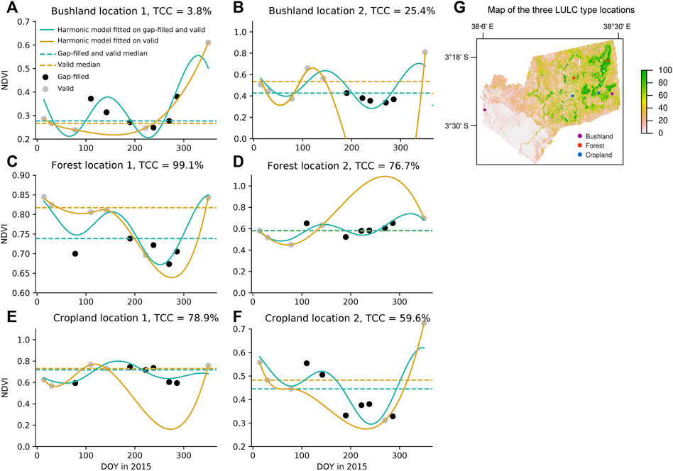
FIGURE 7. Examples of harmonic curves fitted by only valid points (yellow lines) and a combination of MOPSTM gap-filled and valid points (green lines) for NDVI time series across three different land cover types: (A,B) bushland, (C,D) forest, (E,F) cropland, and (G) TCC map of the three land cover type locations. The corresponding color dashed lines are the median of the annual NDVI values. The grey points show the only valid NDVI values and the black points show the MOPSTM gap-filled NDVI values.
Figures 7A,B demonstrate the annual NDVI time series for two bushland pixels with five and six valid observations, respectively. The former had only one trough for the yellow line. The latter had a long period of missing observations between DOY 190 to 286, which resulted in an anomalous trough in the yellow harmonic fit with a bottom NDVI lower than zero during this period. In contrast, the green harmonic fits for both pixels appeared similar and plausible owing to the gap-filled observations. Figures 7C,D illustrate an annual NDVI time series for two forest pixels, which are supposed to have double peaks. Figure 7C had a small trough for the yellow fit due to a missing point on DOY 78. For Figure 7D, an anomalously high yellow harmonic fitted line (over 1.0) occurred due to no valid observations from the DOY 190 to 286. Figures 7E,F indicate NDVI harmonic fitted for two cropland pixels where successive missing points caused a greatly incorrect oscillation in yellow harmonic fits.
3.1.3 Comparisons of the Predictor Variable Importance
The variable importance for the combination of SCs, STMs, and HR coefficients that included MOPSTM gap-filling and did not include gap-filling is compared in Figure 8. The MOPSTM gap-filled variables are always the most important variables, and the MOPSTM gap-filled variables dominated the top 20 variables in the amount. When comparing the same variables, the MOPSTM gap-filled variables had greater importance scores than their non-gap-filled counterparts.
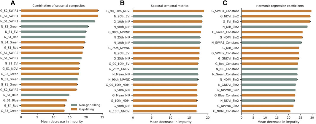
FIGURE 8. Top 20 variable importance measured by mean decrease in accuracy from random forest models using three types of variable predictors: (A) combination of multi SCs, (B) STMs, and (C) HR coefficients. Variables that do not have gap-filling applied start with “N” while variables that have MOPSTM gap-filling applied start with “G”. The importance scores are the mean values for 100 iterations.
3.2 Comparisons of Single-Date Image Experiments
MOPSTM gap-filled pixels performed equivalently to the valid pixels through 121 cross combinations of training and test datasets where the proportions of gap-filled and valid pixels ranged from 0 to 100% (Figure 9). The second row and third column, for example, represent RMSE of the TCC RF model when the training dataset had 10% valid pixels and test dataset had 20% valid pixels. When the proportion of valid pixels was the smallest or the largest in training and test datasets, RMSE was the smallest, which can be observed in the top-left or bottom-right corners in Figure 9. The single-date image acquired from S1 had the smallest RMSE on average while S4 had the largest RMSE on average.
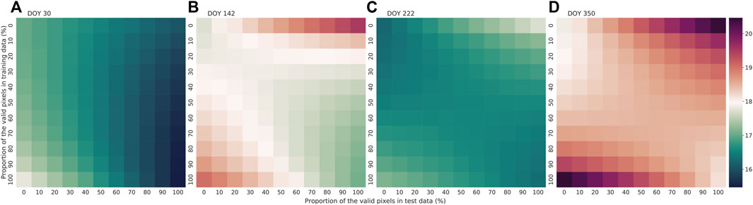
FIGURE 9. RMSE of single-date images from four seasons with respect to different proportions of MOPSTM gap-filled and valid observations involved in both training datasets and test datasets in random forest models. Four Landsat 8 images were acquired from (A) DOY (day of year) 30 in dry and hot season, (B) DOY 142 in long rain season, (C) DOY 222 in dry and cool season, and (D) DOY 350 in short rain season in 2015.
4 Discussion
4.1 Overall Performance of Gap-Filling in TCC
A parsimonious approach to preprocessing, avoiding unnecessary steps, has been recommended for Landsat-based studies (Young et al., 2017). Applying gap-filling in time series analysis makes sense for researchers who use images that are contaminated by sensor failures or clouds and cloud shadows. In this study, we examined TCC modelling to explore the necessity and effectiveness of including gap-filling in the preprocessing step because TCC modelling is an essential measurement in forest management and vegetation growth cycle monitoring and is rarely evaluated for such a purpose. Besides, accurate and time-series maps of TCC are usually limited to the availability of valid observations of the Earth’s surface. Although numerous studies preferred the cloud-free images (Selkowitz, 2010; Yang et al., 2012; Derwin et al., 2020), locations that have persistent cloud cover in rainy seasons, e.g. tropical landscapes, have no valid observations available (Anderson et al., 2010), which becomes a barrier to TCC modelling. Due to the recommendation for preprocessing methods that are well tested, easily available, and sufficiently documented (Young et al., 2017), we chose a hybrid MOPSTM gap-filling method (Tang et al., 2021) for the main examination and a temporal-based method, Steffen spline interpolation as the assistance to explore how the selection of gap-filling method affects TCC modelling results.
We investigated the relative predictive power of TCC models using predictor variables derived from Landsat time series that included gap-filling versus those that did not include gap-filling across a landscape where trees are abundant outside forests. Time series predictors and single-date predictors were used because of their broad applications (Potapov et al., 2015; Halperin et al., 2016; Tong et al., 2017; Brandt et al., 2018; Lister et al., 2020). An overall improvement in RMSE was observed in the models that contained gap-filled predictors on average. Furthermore, the variable importance comparison indicates consistently higher variable importance of MOPSTM gap-filled variables than non-gap-filled variables.
4.2 Comparisons of Time Series Experiments
For SC experiments, the best model without gap-filling was SC in S1, the dry and hot season from January to February. This was partially explained by the variable importance results (Figure 8) where the most important variables were mostly from S1. This finding is in agreement with the previous studies which found that the dry season has the best performance in mapping vegetation attributes (Liu et al., 2016) and characterizing tree, soil, and biodiversity attributes in African savannas (Heiskanen et al., 2017).
Superior performance was observed in SC1 without gap-filling (Figure 4). A possible explanation for this is that the median composite in S1 was of high quality because of the relatively good availability of valid pixels. In contrast, in SC3 and SC4, pixels that were contaminated by clouds and cloud shadows caused great spectral variation and reduced the quality of the median composites derived from the images that were not gap-filled (Figure 5A). Using MOPSTM gap-filling, the median composites in S3 and S4 look smooth and natural (Figure 5C). This can explain why MOPSTM gap-filling had the largest positive effects on SC3 and SC4 predictors. Steffen spline models performed less accurately than non-gap-filling models in S3. Therefore, gap-filling may offer a limited advantage for TCC modelling in cases when median composites can be generated from sufficient valid observations in the time series. Moreover, in some cases, less accurate gap-filling results limited the TCC modelling performance.
Like SCs, gap-filled multi-date images acquired from each season can be potential predictors because these images are cloud-free and possess the same seasonal characteristics as SCs. Therefore, we compared the performance of seasonal gap-filled images (SGIs), labelled as SGI1–SGI4 from S1–S4 (Table 4). Although Steffen spline method delivered larger RMSE for SC1 and SC3 than non-gap-filled results, it had the smaller RMSE for all of the SGIs. Furthermore, MOPSTM yielded the smallest RMSE for SGIs in each season. It supports the great benefit of gap-filled images directly applied in the TCC modelling, even though they are not commonly used. However, using all gap-filled images in a time series to model TCC directly can be costly in calculations and RAM (Belgiu and Drăguţ, 2016) when dozens or hundreds of images are observed in the time series (e.g. including more observations from other satellite sensors). A well-organized implementation in a High Performance Computing environment can resolve the problem (Herrera et al., 2019).

TABLE 4. The median RMSE of seasonal composites (using non-gap-filling, Steffen spline gap-filling, and MOPSTM gap-filling) and seasonal gap-filled images by Steffen spline and MOPSTM methods for modelling tree canopy cover. The highest and lowest values are presented in bold. Abbreviations: SGI: seasonal gap-filled images.
The STMs using MOPSTM gap-filling only showed slight improvement in overall accuracy (Figure 4) while improving for all cases with various numbers of valid observations in Figure 5. Absolute residuals (Figure 6) with respect to the different numbers of valid observations suggest that gap-filled predictor variables had smaller median absolute residuals. RMSE and absolute residuals results, either gap-filled or non-gap-filled, for greater number of observations (e.g. 8–11) were not as good as those for a smaller number of observations (e.g. 5–7), which may be explained by the different distributions of training data selected from the entire pixels that have a specific number of observations. Pixels that have a greater number of valid observations are less likely to occur in montane forests (Nair et al., 2003; Pellikka et al., 2009) where canopy cover is high. Thus, training data selected from these pixels had a poor coverage of the highest TCC areas, resulting in modelling TCC less reliably.
The HR predictor variables without gap-filling surpassed all SCs in TCC modelling (Figure 4), which corroborates with previous results Derwin et al. (2020). HR is capable of mitigating the side effects of the artifacts and noise caused by gaps (Wilson et al., 2018), but the improvement of HR model with gap-filling emphasized the importance of gap-filling, which can fix the harmonic shape of the curve following the expected seasonal pattern of vegetation over the year (Thomas et al., 2021).
The best model in time-series predictors was the combination of SCs with slightly smaller RMSE than that of HR models. The poorer performance of HR may be explained by overfitting in the models, which was a common issue as the maximum number of valid observations was only eleven while the number of harmonic coefficients was five. However, the determination of harmonic terms is a trade-off between the fact that reducing the harmonic terms can help with overfitting and that more harmonic terms are capable of fitting data in dual-rainy-season situation e.g. in the Taita Hills (Brooks et al., 2012; Derwin et al., 2020). Although solving the overfitting effects in HR is beyond the scope of this paper in evaluating the effects of gap-filling in TCC modelling, the improvement from applying gap-filling in HR may help solve the overfitting effects by increasing the number of valid observations (Brooks et al., 2012).
4.3 Comparisons of Single-Date Image Experiments
For single-date predictor experiments, the overall accuracy indicated better performance from using images acquired from the dry seasons than from the wet seasons, which is in line with previous work (Chrysafis et al., 2019, 2017). Furthermore, the results showed that the MOPSTM gap-filled data may have equivalent performance to valid data in terms of TCC modelling accuracy, which was observed from Figure 9. There was no sign that modelling is less accurate using only MOPSTM gap-filled data than using only valid pixels. Figure 9 also suggests that the same proportion of gap-filled pixels in both training and test data is more likely to produce the highest accuracy.
4.4 Different Gap-Filling Methods and Future Perspectives
Between the temporal-based Steffen spline interpolation, and hybrid MOPSTM method, MOPSTM delivered higher accuracy for most of the predictors, except for SC2, a combination of SCs, and HR coefficients (Figure 4). Although both of them had a positive effect on TCC modelling, the strength of the effect varied. In general, a higher accurate gap-filling method (MOPSTM) produced more accurate predictions.
This study only used 1 year of the Landsat time series to model TCC because MOPSTM gap-filling method is proposed to fill gaps over a 1-year period (Tang et al., 2020, 2021) although the method can also use STMs calculated over several years for imputation of missing values. It will be more challenging to examine gap-filling effects for a longer period (Brandt et al., 2018) as few gap-filling methods have been suggested to deliver good performance in a long time series. Further studies can focus on examining other types of gap-filling methods, other predictors, such as best-pixel composites (White et al., 2014), and other downstream tasks, such as land surface temperature monitoring (Li et al., 2013).
5 Conclusion
Landsat data record is a rich resource for time series analysis, like tree canopy cover monitoring, but the lack of appropriate guides in gap-filling, which aims to recover missing observations in images, remains as a barrier to its effective use. To provide a concise guide of the effects of gap-filling on TCC modelling, we used hybrid MOPSTM gap-filling method and temporal-based Steffen spline interpolation to explore how gap-filling affects TCC modelling accuracy. We conclude that gap-filling improves accuracy based on time series SCs, STMs, and HR predictor variables. More accurate the gap-filling method, the greater the positive impact will be on the modelling accuracy. However, when the predictors are derived from sufficient valid observations, gap-filling can be optional. A single MOPSTM-gap-filled image can be an alternative to the original image in terms of TCC modelling.
Data Availability Statement
The original contributions presented in the study are included in the article/supplementary material, further inquiries can be directed to the corresponding author.
Author Contributions
Conceptualization, ZT, JH; methodology, ZT and JH; software, ZT; validation, ZT; formal analysis, ZT; resources, ZT, JH, HA, and PP; data curation, ZT; writing–original draft preparation, ZT; writing–review and editing, ZT, JH, HA, and PP; supervision, PP and JH; project administration, PP, funding acquisition, PP.
Funding
The study was funded by the China Scholarship Council fellowship (Funding No. 201706040079).
Conflict of Interest
The authors declare that the research was conducted in the absence of any commercial or financial relationships that could be construed as a potential conflict of interest.
Publisher’s Note
All claims expressed in this article are solely those of the authors and do not necessarily represent those of their affiliated organizations, or those of the publisher, the editors and the reviewers. Any product that may be evaluated in this article, or claim that may be made by its manufacturer, is not guaranteed or endorsed by the publisher.
Acknowledgments
We acknowledge the support from the Academy of Finland for the SMARTLAND project (Environmental sensing of ecosystem services for developing climate smart landscape framework to improve food security in East Africa), decision number 318645, and from the European Union for the ESSA project (Earth observation and environmental sensing for climate-smart sustainable agropastoral ecosystem transformation in East Africa), FOOD 2020–418–132. We also acknowledge the CSC–IT Center for Science, Finland for its generous provision of computational resources and excellent user support.
References
Acharya, T. D., and Yang, I. (2015). Exploring Landsat 8. Int. J. IT, Eng. Appl. Sci. Res. (IJIEASR) 4, 4–10.
Adhikari, H., Heiskanen, J., Maeda, E. E., and Pellikka, P. K. E. (2016). The Effect of Topographic Normalization on Fractional Tree Cover Mapping in Tropical Mountains: An Assessment Based on Seasonal Landsat Time Series. Int. J. Appl. Earth Observation Geoinformation 52, 20–31. doi:10.1016/j.jag.2016.05.008
Ali, J., Khan, R., Ahmad, N., and Maqsood, I. (2012). Random Forests and Decision Trees. Int. J. Comput. Sci. Issues (IJCSI) 9, 272.
Anchang, J. Y., Prihodko, L., Ji, W., Kumar, S. S., Ross, C. W., Yu, Q., et al. (2020). Toward Operational Mapping of Woody Canopy Cover in Tropical Savannas Using Google Earth Engine. Front. Environ. Sci. 8, 4. doi:10.3389/fenvs.2020.00004
Anderson, L. O., Malhi, Y., Aragão, L. E., Ladle, R., Arai, E., Barbier, N., et al. (2010). Remote Sensing Detection of Droughts in Amazonian Forest Canopies. New Phytol. 187, 733–750. doi:10.1111/j.1469-8137.2010.03355.x
Azzari, G., and Lobell, D. B. (2017). Landsat-based Classification in the Cloud: An Opportunity for a Paradigm Shift in Land Cover Monitoring. Remote Sens. Environ. 202, 64–74. doi:10.1016/j.rse.2017.05.025
Baccini, A., Laporte, N., Goetz, S. J., Sun, M., and Dong, H. (2008). A First Map of Tropical Africa’s Above-Ground Biomass Derived from Satellite Imagery. Environ. Res. Lett. 3, 045011. doi:10.1088/1748-9326/3/4/045011
Belgiu, M., and Drăguţ, L. (2016). Random Forest in Remote Sensing: A Review of Applications and Future Directions. ISPRS J. photogrammetry remote Sens. 114, 24–31. doi:10.1016/j.isprsjprs.2016.01.011
Brandt, M., Rasmussen, K., Hiernaux, P., Herrmann, S., Tucker, C. J., Tong, X., et al. (2018). Reduction of Tree Cover in West African Woodlands and Promotion in Semi-arid Farmlands. Nat. Geosci. 11, 328–333. doi:10.1038/s41561-018-0092-x
Brooks, E. B., Thomas, V. A., Wynne, R. H., and Coulston, J. W. (2012). Fitting the Multitemporal Curve: A Fourier Series Approach to the Missing Data Problem in Remote Sensing Analysis. IEEE Trans. Geoscience Remote Sens. 50, 3340–3353. doi:10.1109/tgrs.2012.2183137
Brooks, E. B., Wynne, R. H., Thomas, V. A., Blinn, C. E., and Coulston, J. W. (2014). On-the-fly Massively Multitemporal Change Detection Using Statistical Quality Control Charts and Landsat Data. IEEE Trans. Geoscience Remote Sens. 52, 3316–3332. doi:10.1109/TGRS.2013.2272545
Brooks, E. (2014). Exponentially Weighted Moving Average Change Detection – Script and Sample Data Blacksburg: Virginia Tech Department of Forest Resources and Environmental Conservation Virginia Tech Department of Forest Resources and Environmental Conservation. doi:10.7294/W4WD3XHK
Campbell, J. B., and Wynne, R. H. (2011). Introduction to Remote Sensing. New York, NY: Guilford Press.
Chaparro, D., Piles, M., Vall-Llossera, M., Camps, A., Konings, A. G., and Entekhabi, D. (2018). L-Band Vegetation Optical Depth Seasonal Metrics for Crop Yield Assessment. Remote Sens. Environ. 212, 249–259. doi:10.1016/j.rse.2018.04.049
Chrysafis, I., Mallinis, G., Gitas, I., and Tsakiri-Strati, M. (2017). Estimating Mediterranean Forest Parameters Using Multi Seasonal Landsat 8 Oli Imagery and an Ensemble Learning Method. Remote Sens. Environ. 199, 154–166. doi:10.1016/j.rse.2017.07.018
Chrysafis, I., Mallinis, G., Tsakiri, M., and Patias, P. (2019). Evaluation of Single-Date and Multi-Seasonal Spatial and Spectral Information of Sentinel-2 Imagery to Assess Growing Stock Volume of a Mediterranean Forest. Int. J. Appl. Earth Observation Geoinformation 77, 1–14. doi:10.1016/j.jag.2018.12.004
Derwin, J. M., Thomas, V. A., Wynne, R. H., Coulston, J. W., Liknes, G. C., Bender, S., et al. (2020). Estimating Tree Canopy Cover Using Harmonic Regression Coefficients Derived from Multitemporal Landsat Data. Int. J. Appl. Earth Observation Geoinformation 86, 101985. doi:10.1016/j.jag.2019.101985
Gitelson, A. A., Kaufman, Y. J., and Merzlyak, M. N. (1996). Use of a Green Channel in Remote Sensing of Global Vegetation from Eos-Modis. Remote Sens. Environ. 58, 289–298. doi:10.1016/s0034-4257(96)00072-7
Halperin, J., LeMay, V., Coops, N., Verchot, L., Marshall, P., and Lochhead, K. (2016). Canopy Cover Estimation in Miombo Woodlands of zambia: Comparison of Landsat 8 Oli versus Rapideye Imagery Using Parametric, Nonparametric, and Semiparametric Methods. Remote Sens. Environ. 179, 170–182. doi:10.1016/j.rse.2016.03.028
Hamrouni, Y., Paillassa, E., Chéret, V., Monteil, C., and Sheeren, D. (2021). From Local to Global: A Transfer Learning-Based Approach for Mapping Poplar Plantations at National Scale Using Sentinel-2. ISPRS J. Photogrammetry Remote Sens. 171, 76–100. doi:10.1016/j.isprsjprs.2020.10.018
Heiskanen, J., Adhikari, H., Piiroinen, R., Packalen, P., and Pellikka, P. K. E. (2019). Do airborne Laser Scanning Biomass Prediction Models Benefit from Landsat Time Series, Hyperspectral Data or Forest Classification in Tropical Mosaic Landscapes? Int. J. Appl. Earth Observation Geoinformation 81, 176–185. doi:10.1016/j.jag.2019.05.017
Heiskanen, J., Liu, J., Valbuena, R., Aynekulu, E., Packalen, P., and Pellikka, P. (2017). Remote Sensing Approach for Spatial Planning of Land Management Interventions in West African Savannas. J. Arid Environ. 140, 29–41. doi:10.1016/j.jaridenv.2016.12.006
Herrera, V. M., Khoshgoftaar, T. M., Villanustre, F., and Furht, B. (2019). Random Forest Implementation and Optimization for Big Data Analytics on Lexisnexis’s High Performance Computing Cluster Platform. J. Big Data 6, 1–36. doi:10.1186/s40537-019-0232-1
Higginbottom, T. P., Symeonakis, E., Meyer, H., and van der Linden, S. (2018). Mapping Fractional Woody Cover in Semi-arid Savannahs Using Multi-Seasonal Composites from Landsat Data. ISPRS J. Photogrammetry Remote Sens. 139, 88–102. doi:10.1016/j.isprsjprs.2018.02.010
Ho, T. K. (1995). “Random Decision Forests,” in Proceedings of 3rd International Conference on Document Analysis and Recognition, 278–282.
Inglada, J., Arias, M., Tardy, B., Hagolle, O., Valero, S., Morin, D., et al. (2015). Assessment of an Operational System for Crop Type Map Production Using High Temporal and Spatial Resolution Satellite Optical Imagery. Remote Sens. 7, 12356–12379. doi:10.3390/rs70912356
James, G., Witten, D., Hastie, T., and Tibshirani, R. (2013). An Introduction to Statistical Learning, 112. New York, NY: Springer New York.
Karlson, M., Ostwald, M., Reese, H., Sanou, J., Tankoano, B., and Mattsson, E. (2015). Mapping Tree Canopy Cover and Aboveground Biomass in Sudano-Sahelian Woodlands Using Landsat 8 and Random Forest. Remote Sens. 7, 10017–10041. doi:10.3390/rs70810017
Kushal, K., Zhao, K., Romanko, M., and Khanal, S. (2021). Assessment of the Spatial and Temporal Patterns of Cover Crops Using Remote Sensing. Remote Sens. 13, 2689. doi:10.3390/rs13142689
Kempeneers, P. (2018). PKTOOLS - Processing Kernel for Geospatial Data Version 2.6.7.6 http://pktools.nongnu.org/html/index.html.
Korhonen, L., Korpela, I., Heiskanen, J., and Maltamo, M. (2011). Airborne Discrete-Return Lidar Data in the Estimation of Vertical Canopy Cover, Angular Canopy Closure and Leaf Area Index. Remote Sens. Environ. 115, 1065–1080. doi:10.1016/j.rse.2010.12.011
Korhonen, L., Packalen, P., and Rautiainen, M. (2017). Comparison of Sentinel-2 and Landsat 8 in the Estimation of Boreal Forest Canopy Cover and Leaf Area Index. Remote Sens. Environ. 195, 259–274. doi:10.1016/j.rse.2017.03.021
Langley, S. K., Cheshire, H. M., and Humes, K. S. (2001). A Comparison of Single Date and Multitemporal Satellite Image Classifications in a Semi-arid Grassland. J. Arid Environ. 49, 401–411. doi:10.1006/jare.2000.0771
Li, Z.-L., Tang, B.-H., Wu, H., Ren, H., Yan, G., Wan, Z., et al. (2013). Satellite-derived Land Surface Temperature: Current Status and Perspectives. Remote Sens. Environ. 131, 14–37. doi:10.1016/j.rse.2012.12.008
Lister, A. J., Andersen, H., Frescino, T., Gatziolis, D., Healey, S., Heath, L. S., et al. (2020). Use of Remote Sensing Data to Improve the Efficiency of National Forest Inventories: A Case Study from the united states National Forest Inventory. Forests 11, 1364. doi:10.3390/f11121364
Liu, H. Q., and Huete, A. (1995). A Feedback Based Modification of the Ndvi to Minimize Canopy Background and Atmospheric Noise. IEEE Trans. geoscience remote Sens. 33, 457–465. doi:10.1109/36.377946
Liu, J., Heiskanen, J., Aynekulu, E., Maeda, E., and Pellikka, P. (2016). Land Cover Characterization in West Sudanian Savannas Using Seasonal Features from Annual Landsat Time Series. Remote Sens. 8, 365. doi:10.3390/rs8050365
Mayes, M. T., Mustard, J. F., and Melillo, J. M. (2015). Forest Cover Change in Miombo Woodlands: Modeling Land Cover of African Dry Tropical Forests with Linear Spectral Mixture Analysis. Remote Sens. Environ. 165, 203–215. doi:10.1016/j.rse.2015.05.006
Margono, B. A., Turubanova, S., Zhuravleva, I., Potapov, P., Tyukavina, A., Baccini, A., et al. (2012). Mapping and Monitoring Deforestation and Forest Degradation in Sumatra (indonesia) Using Landsat Time Series Data Sets from 1990 to 2010. Environ. Res. Lett. 7, 034010. doi:10.1088/1748-9326/7/3/034010
Mclnerney, D., and Kempeneers, P. (2014). “Open Source Geospatial Tools: Applications in Earth Observations,” in Earth Systems Data and Models (Springer).
Moody, A., and Johnson, D. M. (2001). Land-surface Phenologies from Avhrr Using the Discrete Fourier Transform. Remote Sens. Environ. 75, 305–323. doi:10.1016/S0034-4257(00)00175-9
Nair, U. S., Lawton, R. O., Welch, R. M., and Pielke Sr, R. (2003). Impact of Land Use on Costa Rican Tropical Montane Cloud Forests: Sensitivity of Cumulus Cloud Field Characteristics to Lowland Deforestation. J. Geophys. Res. Atmos. 108. doi:10.1029/2001jd001135
Ota, T., Ahmed, O. S., Franklin, S. E., Wulder, M. A., Kajisa, T., Mizoue, N., et al. (2014). Estimation of Airborne Lidar-Derived Tropical Forest Canopy Height Using Landsat Time Series in cambodia. Remote Sens. 6. doi:10.3390/rs61110750
Pellikka, P. K., Clark, B. J., Gosa, A. G., Himberg, N., Hurskainen, P., Maeda, E., et al. (2013). Agricultural Expansion and its Consequences in the Taita Hills, kenya. Dev. Earth Surf. Process. 16, 165–179. doi:10.1016/b978-0-444-59559-1.00013-x
Pellikka, P. K. E., Heikinheimo, V., Hietanen, J., Schäfer, E., Siljander, M., and Heiskanen, J. (2018). Impact of Land Cover Change on Aboveground Carbon Stocks in Afromontane Landscape in kenya. Appl. Geogr. 94, 178–189. doi:10.1016/j.apgeog.2018.03.017
Pellikka, P. K. E., Lötjönen, M., Siljander, M., and Lens, L. (2009). Airborne Remote Sensing of Spatiotemporal Change (1955–2004) in Indigenous and Exotic Forest Cover in the Taita Hills, kenya. Int. J. Appl. Earth Observation Geoinformation 11, 221–232. doi:10.1016/j.jag.2009.02.002
Pflugmacher, D., Rabe, A., Peters, M., and Hostert, P. (2019). Mapping Pan-European Land Cover Using Landsat Spectral-Temporal Metrics and the European Lucas Survey. Remote Sens. Environ. 221, 583–595. doi:10.1016/j.rse.2018.12.001
Poitras, T. B., Villarreal, M. L., Waller, E. K., Nauman, T. W., Miller, M. E., and Duniway, M. C. (2018). Identifying Optimal Remotely-Sensed Variables for Ecosystem Monitoring in colorado Plateau Drylands. J. Arid Environ. 153, 76–87. doi:10.1016/j.jaridenv.2017.12.008
Potapov, P., Li, X., Hernandez-Serna, A., Tyukavina, A., Hansen, M. C., Kommareddy, A., et al. (2020). Mapping Global Forest Canopy Height through Integration of Gedi and Landsat Data. Remote Sens. Environ. 253, 112165. doi:10.1016/j.rse.2020.112165
Potapov, P., Siddiqui, B., Iqbal, Z., Aziz, T., Zzaman, B., Islam, A., et al. (2017). Comprehensive Monitoring of bangladesh Tree Cover inside and outside of Forests, 2000–2014. Environ. Res. Lett. 12, 104015. doi:10.1088/1748-9326/aa84bb
Potapov, P. V., Turubanova, S., Tyukavina, A., Krylov, A., McCarty, J., Radeloff, V., et al. (2015). Eastern Europe’s Forest Cover Dynamics from 1985 to 2012 Quantified from the Full Landsat Archive. Remote Sens. Environ. 159, 28–43. doi:10.1016/j.rse.2014.11.027
Ruefenacht, B. (2016). Comparison of Three Landsat Tm Compositing Methods: a Case Study Using Modeled Tree Canopy Cover. Photogrammetric Eng. Remote Sens. 82, 199–211. doi:10.14358/pers.82.3.199
Schug, F., Frantz, D., Okujeni, A., van Der Linden, S., and Hostert, P. (2020). Mapping Urban-Rural Gradients of Settlements and Vegetation at National Scale Using Sentinel-2 Spectral-Temporal Metrics and Regression-Based Unmixing with Synthetic Training Data. Remote Sens. Environ. 246, 111810. doi:10.1016/j.rse.2020.111810
Selkowitz, D. J. (2010). A Comparison of Multi-Spectral, Multi-Angular, and Multi-Temporal Remote Sensing Datasets for Fractional Shrub Canopy Mapping in Arctic alaska. Remote Sens. Environ. 114, 1338–1352. doi:10.1016/j.rse.2010.01.012
Shataee, S., Kalbi, S., Fallah, A., and Pelz, D. (2012). Forest Attribute Imputation Using Machine-Learning Methods and Aster Data: Comparison of K-Nn, Svr and Random Forest Regression Algorithms. Int. J. remote Sens. 33, 6254–6280. doi:10.1080/01431161.2012.682661
Shen, H., Li, X., Cheng, Q., Zeng, C., Yang, G., Li, H., et al. (2015). Missing Information Reconstruction of Remote Sensing Data: A Technical Review. IEEE Geoscience Remote Sens. Mag. 3, 61–85. doi:10.1109/mgrs.2015.2441912
Souverijns, N., Buchhorn, M., Horion, S., Fensholt, R., Verbeeck, H., Verbesselt, J., et al. (2020). Thirty Years of Land Cover and Fraction Cover Changes over the Sudano-Sahel Using Landsat Time Series. Remote Sens. 12. doi:10.3390/rs12223817
Steffen, M. (1990). A Simple Method for Monotonic Interpolation in One Dimension. Astronomy Astrophysics 239, 443.
Strobl, C., Boulesteix, A.-L., Zeileis, A., and Hothorn, T. (2007). Bias in Random Forest Variable Importance Measures: Illustrations, Sources and a Solution. BMC Bioinforma. 8, 1–21. doi:10.1186/1471-2105-8-25
Tang, Z., Adhikari, H., Pellikka, P. K. E., and Heiskanen, J. (2021). A Method for Predicting Large-Area Missing Observations in Landsat Time Series Using Spectral-Temporal Metrics. Int. J. Appl. Earth Observation Geoinformation 99, 102319. doi:10.1016/j.jag.2021.102319
Tang, Z., Adhikari, H., Pellikka, P., and Heiskanen, J. (2020). “Producing a Gap-free Landsat Time Series for the Taita Hills, Southeastern kenya,” in IGARSS 2020 - 2020 IEEE International Geoscience and Remote Sensing Symposium (IEEE). doi:10.1109/igarss39084.2020.9324671
Tang, Z., Amatulli, G., Pellikka, P. K., and Heiskanen, J. (2022). Spectral Temporal Information for Missing Data Reconstruction (Stimdr) of Landsat Reflectance Time Series. Remote Sens. 14, 172. doi:10.3390/rs14010172
Team, R. C. (2018). R: A Language and Environment for Statistical Computing. Vienna: R Foundation for Statistical Computing.
Teillet, P., Guindon, B., and Goodenough, D. (1982). On the Slope-Aspect Correction of Multispectral Scanner Data. Can. J. Remote Sens. 8, 84–106. doi:10.1080/07038992.1982.10855028
Thomas, V., Wynne, R., Kauffman, J., McCurdy, W., Brooks, E., Thomas, R., et al. (2021). Mapping Thins to Identify Active Forest Management in Southern Pine Plantations Using Landsat Time Series Stacks. Remote Sens. Environ. 252, 112127. doi:10.1016/j.rse.2020.112127
Tong, X., Brandt, M., Hiernaux, P., Herrmann, S. M., Tian, F., Prishchepov, A. V., et al. (2017). Revisiting the Coupling between Ndvi Trends and Cropland Changes in the Sahel Drylands: A Case Study in Western niger. Remote Sens. Environ. 191, 286–296. doi:10.1016/j.rse.2017.01.030
Tucker, C. J. (1979). Red and Photographic Infrared Linear Combinations for Monitoring Vegetation. Remote Sens. Environ. 8, 127–150. doi:10.1016/0034-4257(79)90013-0
Vauhkonen, J., Korpela, I., Maltamo, M., and Tokola, T. (2010). Imputation of Single-Tree Attributes Using Airborne Laser Scanning-Based Height, Intensity, and Alpha Shape Metrics. Remote Sens. Environ. 114, 1263–1276. doi:10.1016/j.rse.2010.01.016
Vogeler, J. C., Braaten, J. D., Slesak, R. A., and Falkowski, M. J. (2018). Extracting the Full Value of the Landsat Archive: Inter-sensor Harmonization for the Mapping of minnesota Forest Canopy Cover (1973–2015). Remote Sens. Environ. 209, 363–374. doi:10.1016/j.rse.2018.02.046
Wang, C., Qi, J., and Cochrane, M. (2005). Assessment of Tropical Forest Degradation with Canopy Fractional Cover from Landsat Etm+ and Ikonos Imagery. Earth Interact. 9, 1–18. doi:10.1175/ei133.1
Wang, S., Azzari, G., and Lobell, D. B. (2019). Crop Type Mapping without Field-Level Labels: Random Forest Transfer and Unsupervised Clustering Techniques. Remote Sens. Environ. 222, 303–317. doi:10.1016/j.rse.2018.12.026
White, J., Wulder, M., Hobart, G., Luther, J., Hermosilla, T., Griffiths, P., et al. (2014). Pixel-based Image Compositing for Large-Area Dense Time Series Applications and Science. Can. J. Remote Sens. 40, 192–212. doi:10.1080/07038992.2014.945827
Wilson, B. T., Knight, J. F., and McRoberts, R. E. (2018). Harmonic Regression of Landsat Time Series for Modeling Attributes from National Forest Inventory Data. ISPRS J. Photogrammetry Remote Sens. 137, 29–46. doi:10.1016/j.isprsjprs.2018.01.006
Yang, J., Weisberg, P. J., and Bristow, N. A. (2012). Landsat Remote Sensing Approaches for Monitoring Long-Term Tree Cover Dynamics in Semi-arid Woodlands: Comparison of Vegetation Indices and Spectral Mixture Analysis. Remote Sens. Environ. 119, 62–71. doi:10.1016/j.rse.2011.12.004
Young, N. E., Anderson, R. S., Chignell, S. M., Vorster, A. G., Lawrence, R., and Evangelista, P. H. (2017). A Survival Guide to Landsat Preprocessing. Ecology 98, 920–932. doi:10.1002/ecy.1730
Zhu, Z., and Woodcock, C. E. (2014). Automated Cloud, Cloud Shadow, and Snow Detection in Multitemporal Landsat Data: An Algorithm Designed Specifically for Monitoring Land Cover Change. Remote Sens. Environ. 152, 217–234. doi:10.1016/j.rse.2014.06.012
Keywords: tropical forest, seasonal composite, machine learning, spectral-temporal metrics, random forest regression, harmonic regression
Citation: Tang Z, Adhikari H, Pellikka PKE and Heiskanen J (2022) Impact of Preprocessing on Tree Canopy Cover Modelling: Does Gap-Filling of Landsat Time Series Improve Modelling Accuracy?. Front. Remote Sens. 3:936194. doi: 10.3389/frsen.2022.936194
Received: 05 May 2022; Accepted: 23 June 2022;
Published: 19 July 2022.
Edited by:
Xiaolin Zhu, Hong Kong Polytechnic University, Hong Kong SAR, ChinaReviewed by:
Jiaqi Tian, National University of Singapore, SingaporeJiayong Liang, New York University, United States
Copyright © 2022 Tang, Adhikari, Pellikka and Heiskanen. This is an open-access article distributed under the terms of the Creative Commons Attribution License (CC BY). The use, distribution or reproduction in other forums is permitted, provided the original author(s) and the copyright owner(s) are credited and that the original publication in this journal is cited, in accordance with accepted academic practice. No use, distribution or reproduction is permitted which does not comply with these terms.
*Correspondence: Zhipeng Tang, emhpcGVuZy50YW5nQGhlbHNpbmtpLmZp