LabSAR, a one-GCP coregistration tool for SAR–InSAR local analysis in high-mountain regions

The coregistration of single-look complex (SLC) SAR images for InSAR or offset tracking applications is often performed by using an accurate DEM and precise orbital information. However, in cold regions, such DEMs are rare over high-latitude areas or not up-to-date over fast melting glaciers for instance. To overcome this difficulty, we propose in this article a coregistration method preserving InSAR phase information that only requires a 3D point of reference instead of a full DEM. Developed in a Python toolbox called LabSAR, the proposed method only uses orbital information to coregister the images on the sphere centered on the Earth center passing by the ground control point (GCP). Thanks to the use of the orbital information, the so-called orbital fringes are compensated without having to estimate them. This coregistration method is compared to other approaches in two different types of applications, InSAR and offset tracking, on a PAZ Dual-Pol Temporal Stack covering the Mont Blanc massif (western European Alps). First, InSAR measurements from LabSAR are compared with the results of the Sentinel-1 ESA toolbox (SNAP). The LabSAR interferograms exhibit clearer topographical fringes, with fewer parameters to set. Second, offset tracking based on LabSAR coregistated images is used to measure the displacement of the Bossons glacier. The results are compared with those obtained by a conventional approach developed in the EFIDIR tools. By evaluating the uncertainties of both approaches using displacements over stable areas and the temporal closure error, similar uncertainty values are found. However, velocity values differ between the two approaches, especially in areas where the altitudes are different from the altitude of the reference point. The difference can reach up to 0.06 m/day, which is in the range of the glacier velocity measurement uncertainty given in the literature. The impact of the altitude of the reference point is limited: this single GCP can be chosen at the median altitude of the study area. The error margin on the knowledge of this altitude is 1,000 m, which is sufficient for the altitude to be considered as known for a wide range of study area in the world.

1 Introduction

The coregistration of images is needed in a broad range of applications in cold or high-mountain regions: SAR backscattering analysis for snow cover mapping (Nagler et al., 2015), DEM construction either using InSAR (Leinss and Bernhard, 2021) or stereoscopy (Brun et al., 2017), and glacier displacement measurement. The latter can be performed with InSAR when the coherence is high enough (Gourmelen et al., 2011) or with offset tracking (Dehecq et al., 2015; Gardner et al., 2018; Millan et al., 2019).

For intensity-only processing where ground rectified detected images (GRD) are used (Leclercq et al., 2021; Scher et al., 2021), the coregistration is performed on a common geographic grid on which all the images are projected. Using a geographic grid also allows the use of a DEM in order to compensate for the impact of the slope in the geometry of the SAR image. However, GRD processing also often implies a multi-look procedure where the phase is discarded, making it unusable for interferometry purposes.

Other approaches more suited for interferometry aim to maintain the phase and achieve a precision of 0.1 pixel during the coregistration. These methods commonly work in two steps, with first a rough coregistration, which can be carried out using offset tracking or ground control points (GCPs), and a second step aiming at the 0.1-pixel precision. This second step can be carried out using multiple approaches such as offset tracking (Wegmuller et al., 1998), the analysis of the linear phase component of the SAR PSF (Scheiber and Moreira, 2000) or optical flow (Plyer et al., 2015). In order to perform finer coregistration without these two steps, it is possible to perform a DEM-assisted coregistration as for example in Petillot et al. (2010) or in Nitti et al. (2008). However, having a fine up-to-date DEM can be complicated, mostly in high and low latitudes, which are not covered by SRTM acquisition and more difficult to image with optical sensors or because changes such as glacier melt make the DEM quickly obsolete (Altena and Kääb, 2017).

In order to have a coregistration tool that can be used for multiple SAR sensors while preserving the phase information, LabSAR coregistation was developed, using a minimal number of auxiliary parameters and no image information. The principle used in LabSAR for SAR image coregistration was already demonstrated in Nicolas et al. (2012) by the construction of a TerraSAR-X/Cosmo-SkyMed interferogram. In LabSAR, it has been extented to a spherical grid, closer to the ellipsoid, parameterized by only one geographical point. All the other parameters are read directly from the auxiliary files. Image processing tools such as denoising or interferogram formation and visualization functions are also included in the toolbox. The toolbox is coded in Python in order to be easily used with any computer and updated when new sensors are launched.

In order to evaluate LabSAR approach, we compared it to two state-of-the-art approaches:

• SNAP: the Sentinel-1 ESA toolbox, which proposes two steps coregistration based on ground control points and offset tracking.

• EFIDIR: a displacement estimation toolbox, which uses a DEM-based geolocalization of SAR pixels.

The three methods are described in Section 2.

The comparison is performed over the Chamonix Mont Blanc test site, in the western European Alps. Two study areas, presented in Section 3, are selected:

• The city of Chamonix, which exhibits many point-like scatterers with a high degree of coherence. These two characteristics facilitate the evaluation first of the coregistration and second of the InSAR phase quality.

• The Bossons glacier, close to Chamonix, which is an ideal test area for offset tracking methods due to the large displacement (about 50 cm/day) and the multiple crevasses (Fallourd et al.,2011).

In Section 4, the coregistration is evaluated on the intensity image. In Section 5, InSAR evaluation is performed. Finally in Section 6, the displacement estimation after LabSAR coregistration is evaluated.

2 Methods

2.1 LabSAR

LabSAR is a platform coded in Python that offers coregistration for SAR images from different satellites such as TerraSAR-X (TSX), TanDEM-X (TDX), PAZ and Cosmo-SkyMed images in X-band, Sentinel-1 images in C-band, and ALOS PALSAR images in L-band, as long as the images are synthesized in zero-Doppler configuration.

LabSAR works with only a limited set of auxiliary data. In stripmap mode, these parameters are the satellite trajectory (time, position, and velocity), the pixel spacing in azimuth and range, equivalent to the pulse repetition frequency (PRF) and range sampling frequency (RSF) in the time domain, and the time of the first sample in range t₀. Auxiliary data are extracted from each sensor auxiliary files, thus LabSAR can be used for all the aforementioned sensors.

The first step in LabSAR approach is to compute a Virtual Geographic Coordinate Grid (VGCG) corresponding to the main image I_m (r, a), on which the secondary images are going to be coregistered. The VGCG is constructed on a sphere, which radius corresponds to the distance of the GCP to the Earth center. The direction and the sampling of the grid axes correspond to the azimuth and the range axes of the main image, as sketched in Figure 1.

FIGURE 1

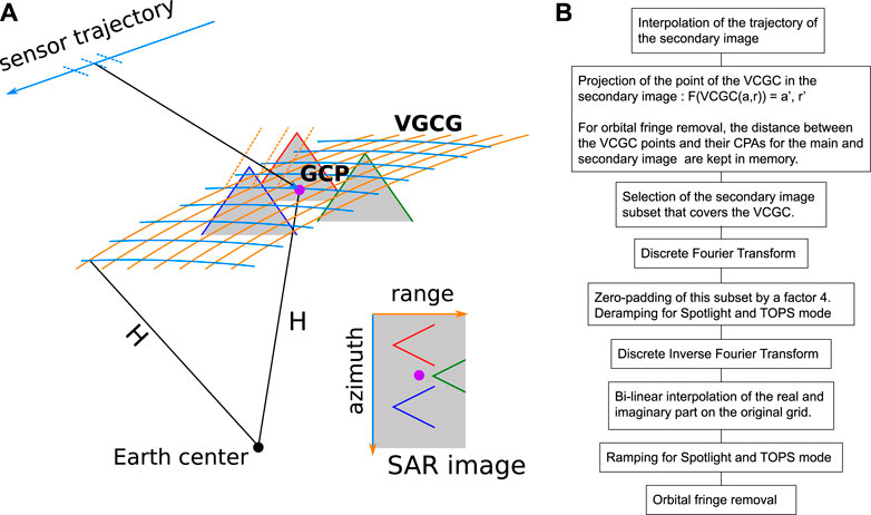
FIGURE 1. (A) Schematic view of the Virtual Geographic Coordinate Grid (VGCG) and the projection in the SAR image. The relief is represented by the red, green, and blue mountains. The ground control point (GCP) is represented in violet. It is at the center of the resampled SAR image subset. The VGCG is constructed on a sphere, centered on the Earth center and whose radius is the distance between the GCP and the Earth center. The grid itself is defined by the range lines in orange, parallel to the sensor trajectory and spaced by the ground range sampling, and the azimuth lines in light blue, parallel to the ground range direction and spaced by the azimuth sampling. (B) LabSAR coregistration processing chain.

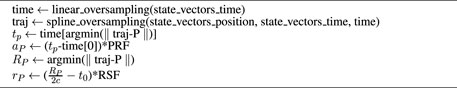
The computation of pixel location r_P, a_P in the SAR image I (r, a) of a given geographic coordinate P = [x, y, z] is performed by the transformation L_I. The process corresponds to the following Algorithm 1. It starts with the computation of Closest Point of Approach (CPA) of P to the satellite orbit, that is, by computing the minimum of the distance between the considered geographic location and the discrete trajectory. Because the trajectory is given by a limited number of state vectors, the time of acquisition (state_vectors_time) is linearly oversampled to get the CPA, with a subpixelic precision (function linear_oversampling). The satellite position (state_vectors_position) is oversampled at the same step using a spline of degree 3, for each spatial component independently (function spline_oversampling). Then, the CPA position is converted in pixel position in range and azimuth (r_P, a_P). For the azimuth, the CPA time t_p is subtracted by the time at the start of the trajectory and multiplied by the PRF. For the range, the CPA distance R_p is converted in time using the speed of light c and subtracted by the time of the first sample in range before being multiplied by the RSF. By construction, the location in the main image I_m (r, a) of the VGCG points, are the center of the pixels: $L_{I_m}(VGCG(r,a))=r,a$.

Algorithm 1. the function L_I that compute the location r_P, a_P in the image I (r, a) of the point P = [x, y, z]

To coregister the secondary image, the following steps summarized in Figure 1 are used:

1) Projection of all the points of the VGCG in the secondary images using $L_{I_s}$. In most cases, the corresponding pixel locations are not integers and image resampling is necessary.

2) Selection of the image subset which covers the VGCG, by computing the minimum and maximum azimuth and range pixel position of all the points in the grid.

3) Resampling of the secondary subset. This is performed in two steps. First, the subset is oversampled using zero-padding by a factor 4. This Shannon oversampling preserves the direction of the phase by taking into account the sensor PRF. Moreover, during this oversampling, the deramping, necessary for spotlight or TOPS modes, can be performed. It requires complementary auxiliary data such as the minimum and maximum steering angles. After this Shannon oversampling, the oversampled subset is resampled over the pixel position of the main image by a bi-linear interpolation of the real and imaginary part followed by the ramping. This succession of spectral and temporal interpolation allows for a compromise between the memory required by the spectral interpolation and the time required by the spatial interpolation. Moreover, it allows for a coregistration of an ascending image over a descending one or of images of different sensors

For interferometric processing, orbital fringes can be compensated during the resampling by the computation of the difference of the distance between each point of the VGCG and their CPA for the main and secondary images.

This coregistration process would be usable over any geographical grid. However, the choice of a geographical grid with a fix step in a geographic coordinate reference system (CRS) can be problematic over strong relief areas such as the Chamonix valley used in this work. The size of the pixel on the ground exhibits strong variations with the local incidence angle. To obtain a ground sampling that verifies Shannon theorem in areas of slopes facing the sensor, the sampling step of the grid has to be very small, creating an oversampling in flat areas or areas of slopes in the opposite direction of the sensor. With the VGCG choice performed in LabSAR, the coregistration of a secondary image acquired under interferometric conditions, will only result in very small under or oversampling because of the change in incidence angle between the two images. Furthermore, in local denoising or during the interferometric processing where the size in pixels of the processing window is constant, the number of independent pixels in the processing window is constant over the image. On the contrary, using a constant window size in meter over a geographical grid would make the number of looks vary within the image depending on the relief.

However, since it is possible to convert any geographic location in pixel location knowing the trajectory of the satellite during the main image acquisition, LabSAR can also be used to project an external DEM into the image and get a look-up table (LUT) giving the 3D geographic coordinates of every pixel of the original image and enabling layover detection.

2.2 EFIDIR tools

The EFIDIR toolbox has been developed during the EFIDIR project (Extraction and Fusion of Information for ground Displacement measurements with Radar Imagery, https://efidir.poleterresolide.fr/). It is dedicated to the processing of optical and SAR images for the measurement of surface displacement by offset tracking (Ponton et al., 2014; Benoit et al., 2015). The proposed pipeline for SAR images is based on the use of an accurate DEM and the orbital and sensor information to perform the following steps:

1) the geocoding (latitude, longitude, and elevation) of the pixels of the SAR images and the “radarcoding” (range and azimuth coordinates) of the pixels of the DEM grid in different SAR images (Petillot et al., 2010);

2) the crop of the different SAR images based on the min–max range and azimuth coordinates for the studied area, which provides a rough coregistration of the SAR images without any resampling;

3) the computation of range and azimuth offset maps by cross-correlation between these roughly coregistered SAR images. Subpixel offsets are measured by a fast implementation of the normalized cross-correlation in the spatial domain followed by a parabolic interpolation of the correlation pick (Vernier et al., 2011). These initial offset maps measure i) the stereoscopic effect due to the topography and the baseline between the two orbits and ii) the surface displacement between the two acquisitions;

4) the subtraction of the residual offsets due to the stereoscopic effect, which can be computed directly from the DEM and the two satellite orbits. The corrected offset maps are then transformed into velocity maps, which measure the projection of the surface velocity on the line of sight (LOS) and azimuth directions (Fallourd et al., 2011).

In Section 6, the EFIDIR tools are used to compare the offset tracking results obtained by two different approaches on fast moving glaciers:

1) by using LabSAR with a single GCP for coregistration of the secondary SAR image on the main SAR image. Then, offsets are measured with EFIDIR cross-correlation tools and directly converted into range/azimuth velocity maps;

2) by using the whole EFIDIR pipeline which avoids the resampling of the secondary SAR image, but requires an accurate DEM over the studied area.

2.3 SNAP approach

SNAP coregistration has been carried on using the Snappy, the Python API of SNAP. The coregistration steps are the followings:

1) The subsets extraction, for each image in the temporal stack. This subset is defined with the same pixel bounding box to have exactly the same subset for the main image as in LabSAR.

2) The stack creation, to apply the processing to all the images.

3) The coregistration, which is divided in two steps:

a) The computation of the position of the main ground control points (GCPs) in the secondary images. An approximated position of the GCPs is first computed using geometrical information, and then refined using cross-correlation of patches around the GCPs.

b) The warping which corresponds to the extrapolation of the offsets between main and secondary GCPs based on a polynomial function.

By extracting the complex values at this step, it is already possible to obtain an interferogram. However, this interferogram exhibits orbital fringes.

4) The interferogram formation, during which the orbital fringes can be estimated as a polynomial function using the knowledge of the trajectory and the ellipsoid. As for the coregistration, only a subset of points are used for this estimation, and then interpolated over the whole image.

Apart from the size of the interferogram window, we used the default parameters for all the SNAP functions.

3 Data and study area

To evaluate the performances of LabSAR, areas with steep relief in the French Alps have been chosen. For the interferometric evaluation, the test site is the city of Chamonix, which exhibits a good coherence. For the displacement estimation, the test site is the Bossons glacier. It is characterized by a steep slope and numerous crevasses, which can easily be tracked by offset tracking. The surface velocity of the glacier is on average of about 80 cm/day and at the maximum of 2 m/day, leading to a low interferometric coherence.

The images used are acquired by the satellite PAZ in stripmap mode. PAZ is a Spanish high-resolution X-band SAR sensor with a repeat cycle of 11 days. The spatial spacing is about 2 m in SAR geometry. The configuration of the satellite is very similar to TerraSAR-X configuration. The polarizations of the images are HH and HV. The three consecutive images used in this study are acquired on 28/09/2020, 09/10/2020, and 20/10/2020. The first image is used as the main image for interferometry. For the city of Chamonix, the GCP altitude is 1,034 m, while for the Bossons glacier, the GCP altitude is initially 2,601 m. The images, overlaid on an optical image, are shown in Figure 2. The image over the Bossons glacier has 3,799 pixels in range and 3,540 pixels in azimuth, while the image over the Chamonix area has 1,002 pixels in range and 1,908 pixels in azimuth. The interferometric configurations for the two interferometric pairs are really close, as summarized in Table 1.

FIGURE 2

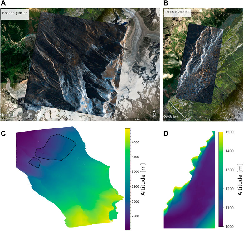
FIGURE 2. (A,B) Overlay of the PAZ image on the optic image covering the Bossons glacier (A) and Chamonix (B). The PAZ image is a temporal mean of the three images studied here, displayed in amplitude with the HH channel in orange and the HV channel in blue. The same threshold is used for the visualization of both polarimetric channels (computed as μ + 3σ from the mean μ and the standard deviation σ of the amplitude of both images). Small amplitude differences due to building orientation can be seen in the Chamonix image. (C,D) Altitude for each pixel of the SAR images over the Bossons glacier (C) and the Chamonix area (D). On the Bossons glacier DEM, the black polygons correspond to the stable areas used in Section 6.3 to study the influence of the central point altitude.

TABLE 1

TABLE 1. Summary of the two interferometric configurations. The ambiguity height is computed using the PAZ acquisition parameters: an altitude of 514 km, a mean incidence angle of 37.86°, and a wavelength of 3.1 cm.

For both areas, we also computed the altitude for each pixel. For the Chamonix area, the goal was to get the altitude of the pixels having a high-coherence value. To do so we projected the IGN (French National Geographic Institute) RGE-Alti DEM pixels below 1,500 m on the SAR images. Since the spacing of the DEM is 1 m, multiple geographic points can be projected in the same pixel. When that was the case, we took the mean altitude in the pixels to construct our projected DEM. We interpolated linearly for the pixels where no geographic points were projected. The altitude obtained for each pixel is represented in Figure 2.

4 Application of LabSAR for amplitude comparison

In order to evaluate the coregistration capacity of LabSAR, we compared the SNAP coregistration, LabSAR coregistration, and the image without any coregistration as the latter would be used in the EFIDIR framework. The results are presented in Figure 3. For the image acquired on 28/09/2020, that is, the main image, the pixel intensity was exactly the same for the three images because the main image was not coregistered using both LabSAR and SNAP.

FIGURE 3

FIGURE 3. Color composition of the intensity of the coregistered image at the same date. Red: the original image as used in the EFIDIR framework, green: LabSAR, and blue: SNAP. (A,D,G) 28/09/2020 image, (B,E,H) 09/10/2020 image, and (C,F,I) 20/10/2020 image. (A–C) Full image (D–F) zoom on three point-like scatterers in the city of Chamonix (G–I) zoom on a speckle area due to the mountain layover. Since the main image has not been resampled with any of the frameworks, the (A,D,G) images are in grayscale.

In Figure 3, we can note the absence of data on SNAP image on the east side (right) for the 09/10/2020 image and on the west side (left) for the 20/10/2020 image, due to the selection of the pixel bounding box in the SNAP pipeline before the coregistration process.

One of the main difference between SNAP and LabSAR is that SNAP coregistration varies on the image, while LabSAR displacement are more global since they only depends on the difference in the acquisition geometry. On the 09/10/2020 image, we can see that for point-like scatterers (Figure 3E), LabSAR and SNAP coregistrations are very close (red–cyan), while for textured speckle (Figure 3H), SNAP is closer to the original image than to LabSAR coregistration (magenta-green). For the 20/10/2020 image, the point-like scatters (Figure 3F) are coregistered differently between LabSAR and SNAP (red–green–blue), while the texture speckle (Figure 3I) is coregistrated similarly between SNAP and LabSAR (red–cyan).

In order to compare the quality of the coregistration, we also compared the coregistrated secondary images to the main image. This comparison is presented in Figure 4. On the full image, a lot of little differences due to the speckle or small target changes can be seen, but no large areas of changes can be observed. When looking at the point-like scatterers comparison, we can see that the secondary images coregistered with SNAP exhibit a larger shift that the one coregistrated with LabSAR. On the 20/10/2020 image (Figure 4F) and h), the SNAP shift is close to 1 pixel in the azimuth direction for most of the point-like scatterers in the image.

FIGURE 4

FIGURE 4. Intensity of the coregistered secondary image on the main image. Orange: the main image and blue: the secondary image (A,E) LabSAR: the secondary 09/10/2020 vs. the main 28/09/2020 image, (B,F) LabSAR: the secondary 20/10/2020 vs. the main 28/09/2020 image, (C,G) SNAP: the secondary 09/10/2020 vs. the main 28/09/2020 image, (D,H) SNAP: the secondary 20/10/2020 vs. the main 28/09/2020 image. (A–D) Full image (E–H) zoom on three point-like scatterers in the city of Chamonix.

5 Application of LabSAR for InSAR fringe estimation

5.1 Evaluation of the phase quality

To evaluate the quality of the InSAR phase after coregistration, we compare the measured phase ϕ to a reference phase ϕ_ref.

If the reference phase depends only on the topography, we use the following equation:

${\varphi }_{\mathit{ref}}=k_{z}h=\frac{4\pi }{\lambda }\frac{B_{\perp }}{H\tan \left(\theta \right)}h,(1)$

where h is the altitude of each point, λ is the wavelength, B_⊥ is the perpendicular baseline, H is the satellite altitude, and θ is the incidence angle. All the values of these parameters are given in Section 3.

If we include the orbital fringes, the phase reference formula from Equation 1 becomes:

${\varphi }_{\mathit{ref}}=k_{z}h+{\varphi }_o=\frac{4\pi }{\lambda }\frac{B_{\perp }}{H\tan \left(\theta \right)}h+\frac{4\pi }{\lambda }\left(d_{s,g}-d_{m,g}\right),(2)$

where d_s,g is the distance between the secondary orbit and the grid, while d_m,g is the distance between the main orbit and the grid.

Since the phase is wrapped modulo 2π, we assess the concentration and the bias of the histograms using directional statistics (Kanti and Mardia 1999). The concentration is measured by the mean resultant length R ∈ [0, 1] of the phase difference distribution, and the bias is measured by the mean phase μ, both defined in the following equation:

${Re}^{i\mu }=\frac{1}{N}\sum _{k=0}^{N-1}{e}^{i\left({\varphi }_k-{\varphi }_{\mathit{ref,k}}\right)}.(3)$

For mono-modal histograms as the ones found in this study, the more concentrated the histograms are, the closer the R is to 1. The computation of R and μ is carried out over all the pixels where the height is available. However, since SNAP coregistration may vary in the image, we also measure the concentration of the phase difference over a high coherence area, to ensure a good coregistration. These pixels are selected with a coherence γ > 0.8.

5.2 Results before orbital fringes removal

To evaluate LabSAR interferometric capacity, we computed the interferogram of the main image and the two secondary images after coregistration and compared them to the interferograms obtained with SNAP. Since SNAP interferogram processing chain works in two steps: image matching followed by orbital fringe removal during the interferogram formation, we have first compared the image matching step of SNAP to the coregistration without orbital fringes removal of LabSAR. All the interferograms have been formed using a 5 × 5 sliding window.

Figure 5 represents the reference phase that follows Eq. 2, as well the measured phase and the coherence for both methods and both image pairs. The maps of the coherence are very close between LabSAR and SNAP. The coherence is high over the city and low over the mountain sides. The coherence histograms, represented in Figure 6, confirm the similar coherence value of both methods. For the 20/09/2020 and 20/10/2020 image pairs, the coherence computed with the LabSAR processing chain exhibits a bit more pixels with a degree coherence above 0.9 than the one computed using SNAP.

FIGURE 5

FIGURE 5. Coherence and phase of the interferogram before obrital fringes removal. (A–D) coherence and (E–J) phase of the interferograms (A,B,E,F,G) between the 28/09/2020 and 09/10/2020 images. (C,D,H,I,J) between the 28/09/2020 and 20/10/2020 images. (E,H) simulated phase, (A,C,F,I) SNAP resampling. (B,D,G,J) LabSAR resampling.

FIGURE 6

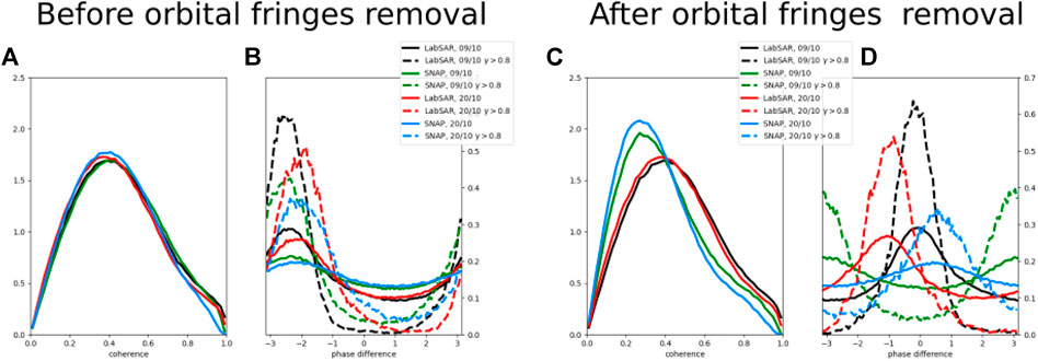
FIGURE 6. (A) Histograms of the coherence for the four interferograms after orbital fringes removal. (B) Histogram of the pixel-wise comparison of the measure phase and the reference phase obtained from the height of the area, with orbital fringe removal—the entire image − − pixel with a coherence above 0.8. (C) Histograms of the coherence for the four interferograms before orbital fringes removal. (D) Histogram of the pixel-wise comparison of the measure phase and the reference phase obtained from the height of the area, without orbital fringe removal—the entire image − − pixel with a coherence above 0.8. Interferogram between the 20/09/2020 image and 09/10/2020 coregistered with LabSAR, interferogram between the 20/09/2020 image and 20/10/2020 coregistered with LabSAR, interferogram between the 20/09/2020 image and 09/10/2020 coregistered with SNAP, and interferogram between the 20/09/2020 image and 20/10/2020 coregistered with SNAP.

Even if the value of the degree of coherence are similar, the phase computed with the LabSAR processing chain shows clearer fringes, as it can be seen in Figure 5. This can also be seen in the pixel-wise difference between the reference phase and the phase measure with both methods. Their histograms, represented in Figure 7, show a good correspondence between the reference phase and the phase measured both by SNAP and LabSAR, but the histogram of the phase measured with the LabSAR processing chain is more concentrated: the mode counts a higher number of pixels and the number of pixels outside the main lobe is lower. This is confirmed by the mean resultant length R, which is higher for LabSAR as summarized in Table 2, even for areas of high degree of coherence (γ > 0.8). The offset between the reference phase and the measured one, reflected in the value the main lobe of the histogram, is due to the choice of the reference phase value at the altitude zero. The offset value, computed using the μ parameter is very close for both methods and both image pairs, as summarized in Table 2.

TABLE 2

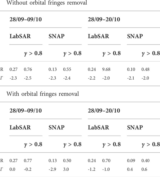
TABLE 2. Statistics of the histograms of the pixel-wise comparison between the measured phase and the reference phase, obtained from the projected altitude and the sensor information.

FIGURE 7

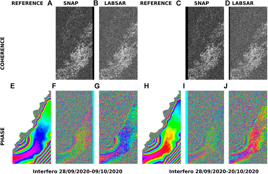
FIGURE 7. Coherence and phase of the interferogram after obrital fringes removal. (A–D) coherence and (E–J) phase of the interferograms. (A,B,E,F,G) between the 28/09/2020 and 09/10/2020 images. (C,D,H,I,J) between the 28/09/2020 and 20/10/2020 images. (E,H) simulated phase, (A,C,F,I) SNAP resampling, and (B,D,G,J) the LabSAR resampling.

5.3 Results after orbital fringes removal

After the evaluation without orbital fringes removal, we compared the full interferometric processing chain of LabSAR and SNAP, with again a 5 × 5 sliding window for both methods.

The histograms of LabSAR coherence presented in Figure 6 have the same shape with and without orbital fringes removal, while the SNAP coherence histograms show fewer high coherence pixels with the orbital fringes removal. On the coherence maps represented in Figure 7, this results in a higher contrast between the high coherence and the low coherence pixels in the city.

Also Figure 7 shows that the phase computed from LabSAR coregistration again exhibits clearer fringes, but that no fringes are visible outside of the valley with both methods. The histogram of differences between the measured phase and the reference topographic phase from Equation 1 are represented in Figure 6B where it can be seen that LabSAR exhibits a more concentrated histogram for both interferograms. The coherence decrease due to the removal of the orbital fringes in SNAP, results in a slight spread of the histogram of the pixel-wise difference between the reference phase and SNAP estimated phase, as shown by the mean resultant length of the phase distribution summarized in Table 2.

The phase difference histograms represented in Figure 6B as well as the computation of the parameter μ summarized in Table 2 shows that there is a bias between SNAP and the reference phase due to the choice of the value of the phase at the reference altitude. Since the VGCG is being constructed on the main image, we expected no phase bias due to the choice of the reference altitude using LabSAR methods. However, a bias, seen on the interferograms between the 28/09/2020 and 20/10/2020 images, could come from a phase screen due to the atmospheric effect.

This experiment shows that the LabSAR pipeline, which encompasses a pixel-wise coregistration computed from orbital information, leads to clearer fringes than the two steps SNAP coregistration. It also shows that the orbital fringe compensation by the satellite-to-grid distance measurement before interferogram formation yield a higher coherence that the one performed by the estimation of a polynomial function as performed in SNAP.

6 Application of LabSAR for displacements estimation using offset tracking

In the two previous sections, we evaluated LabSAR capacities for InSAR applications. Nevertheless, the estimation of displacement by offset tracking is also very important to better understand glacier evolution in areas where the surface changes are very fast to preserve the coherence. In this section, we evaluate LabSAR capacities to measure displacements over the Bossons glacier where no fringes are visible after coregistration with both SNAP and LabSAR because of a low coherence.

To do so, we compared two different pipelines: 1) a coregistration with LabSAR followed by the EFIDIR offset tracking and 2) the full EFIDIR pipeline detailed in Section 2.2. For both pipelines, the displacement is computed using the EFIDIR tools, with a square correlation window of 105 pixels. The square search window is of 135 pixels, allowing a maximum displacement of 15 pixels, which corresponds to 30 m for PAZ images.

6.1 Uncertainty evaluation

The uncertainty of the velocity measurements using both LabSAR and EFIDIR approaches is evaluated first by comparing the value of velocities computed over stable ground and then by comparing the temporal closure of the displacements.

6.1.1 Displacements over stable ground

To evaluate the uncertainty, we compute the displacement over stable ground, which should be equal to zero in the ideal case. The selected regions are represented in Figure 8.

FIGURE 8

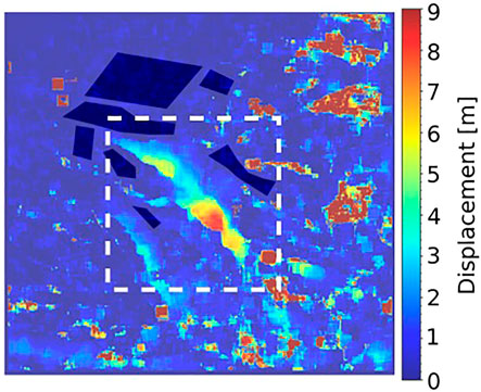
FIGURE 8. Dark blue polygons correspond to the stable areas selected to compare LabSAR and EFIDIR uncertainties. It is superimposed over displacement magnitudes between the 28/09/2020 and 09/10/2020 images. These displacements have been computed with the full EFIDIR pipeline in m and are represented with colors ranging from blue to red. The outliers have not been filtered out for this study and appear in dark red: they are due to temporal decorrelation, lack of feature or point target due to cars (north-west).

Three criteria are defined to quantify the errors: the root mean square error (RMSE), mean error (ME), and standard deviation (std) of the velocity over stable ground. The velocity between dates t₁ and t₂ is computed from the displacement between dates t₁ and t₂ as ${\vec{v}}_{t_1/t_2}(i,j)=\frac{1}{t_2-t_1}{\vec{d}}_{t_1/t_2}(i,j)$. Because the expected velocity value is zero over stable ground, the three criteria are formulated as:

$RMSE=\sqrt{{mean}_{\left(i,j\right)\in {\omega }_1}\left[v{\left(i,j\right)}^2\right]},(4)$

$ME={mean}_{\left(i,j\right)\in {\omega }_1}\left[v\left(i,j\right)\right],(5)$

$std=\sqrt{{mean}_{\left(i,j\right)\in {\omega }_1}\left[{\left(v\left(i,j\right)-ME\right)}^2\right]}.(6)$

In these formulas v (i, j) stands for either the azimuth velocity, the slant-range velocity, or the velocity magnitude over the pixel (i, j), ω₁ corresponds to ice-free areas defined by the dark blue polygons in Figure 8. The velocity is computed between the images acquired on 28/09/2020 and 09/10/2020.

The RMSE measures the distance between the expected and the observed values. It penalizes large errors. The ME measures the bias of the velocity measurements, while the std corresponds to the dispersion of the velocity measurements over stable ground. Note that if the bias is null, the RMSE and the std are equal.

Table 3 highlights that the RMSE, ME, and std over stable ground are roughly similar between LabSAR and EFIDIR approaches. The differences are on the order of 1 cm/day: the RMSE of the velocity magnitude is 0.01 m/day lower for the LabSAR approach than for the EFIDIR approach. Note that the criterion is larger for velocity magnitude than for the two velocity components because positive and negative values do not compensate in this case.

TABLE 3

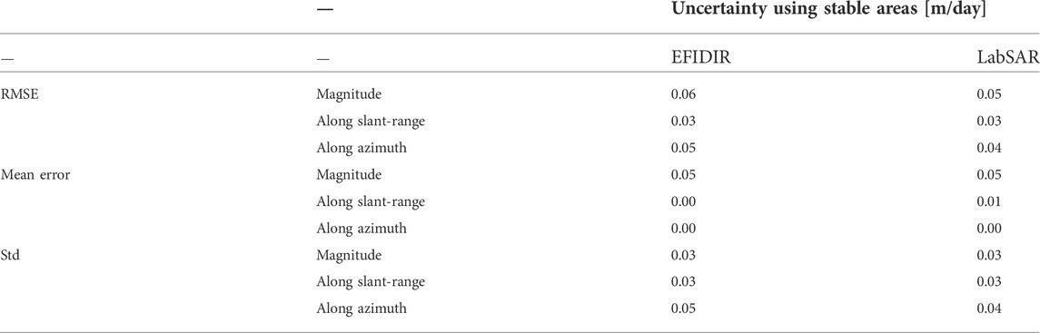
TABLE 3. Comparison of the RMSE, ME, and std of the velocity magnitude, slant-range velocity, and azimuth velocity computed over stable ground using the EFIDIR and LabSAR approaches. The results are in m/day.

This experiment shows that there was no leftover in LabSAR coregistration that could create a bias, as also shown in Section 4.

6.1.2 Temporal closure

Because the uncertainty estimated using off-glacier displacements can be underestimated (Altena et al.,2021), we also compared the temporal closure error using both approaches. The temporal closure error is formulated for each pixel (i,j) in m/day as:

$\overrightarrow{ϵ\left(i,j\right)}=\frac{1}{t_3-t_1}\left({\vec{d}}_{t_1/t_3}\left(i,j\right)-\left({\vec{d}}_{t_1/t_2}\left(i,j\right)+{\vec{d}}_{t_2/t_3}\left(i,j\right)\right)\right),(7)$

with ${\vec{d}}_{t_l/t_m}(i,j)$ the displacement between the dates t_l and t_m over the pixel (i, j). The three dates t₁, t₂, and t₃ used for this analysis are: 28 September 2020, 9 October 2020, and 20 October 2020, respectively.

If there were no errors in the velocity computation, the temporal closure should be equal to zero. Two criteria are defined to measure the error and the dispersion of the temporal closure: the median error (MdE) and the median absolute deviation (MAD), defined as:

$MdE={median}_{\left(i,j\right)\in {\omega }_2}\left[ϵ\left(i,j\right)\right],(8)$

$MAD={median}_{\left(i,j\right)\in {\omega }_2}\left[|ϵ\left(i,j\right)-{mean}_{\left(i,j\right)\in {\omega }_2}\left[ϵ\left(i,j\right)|\right]\right],(9)$

where ϵ(i, j) stands for either the temporal closure error of azimuth displacement and slant-range displacement or the norm of the temporal closure of the displacements over the pixel (i, j), ω₂ corresponds to the study area over the Bossons glacier shown in Figure 2. Indeed, the MdE is a robust estimation of the bias of the measurement and the MAD is a robust estimation of the dispersion of the error.

It can be seen on Table 4 that the MdE and MAD of the temporal closure error are equal between LabSAR and EFIDIR approaches for the slant-range velocities and the norm of the temporal closure. However, the bias of the azimuth velocities is 0.02 m/day higher for the LabSAR approach than the EFIDIR approach, while the dispersion of the error is 0.01 m/day lower for the LabSAR approach than the EFIDIR approach. Moreover, it can be noticed in Figure 9 that the highest temporal closure errors are recorded in the large gradient areas such as the border of the glacier. This is due to the use of a rigid correlation window: at the border of the glacier, the correlation window covers both the glacier and the stable ground, which can lead to an underestimation of the displacements.

TABLE 4

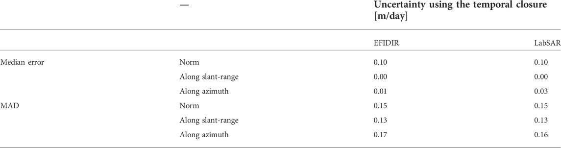
TABLE 4. Comparison of the MAD and MdE of the temporal closure of the displacements for the slant-range and azimuth direction computed using the EFIDIR and LabSAR approaches. The norm corresponds to the norm of the temporal closure error vector defined in Eq. 7. The results are in m/day.

FIGURE 9

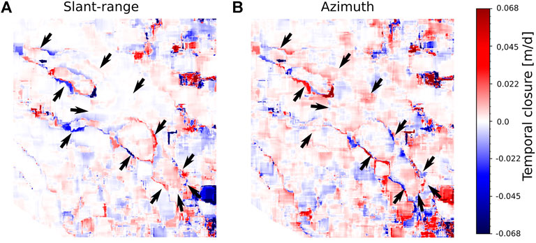
FIGURE 9. Temporal closure error for the LabSAR approach along (A) slant-range direction and (B) the azimuth direction in m/d. The area shown is in the white rectangle represented in Panel 8. The black arrows represent the borders of the glacier that exhibit the high temporal closure absolute value.

In conclusion, the comparison of the displacements over stable areas and the temporal closure error shows that both approaches have similar uncertainties.

6.2 Difference in velocity values over the study area

Even if the uncertainty between the two approaches is of the same order of magnitude, the value of the displacement is not the same.

Figure 10 shows the difference between velocity measurements from LabSAR and EFIDIR approaches along slant-range and azimuth directions. The differences which can be observed in the slant-range direction reveal the effect of using the altitude of a unique reference point to build the LabSAR grid. Because the reference point is located in the middle of the study area, the differences between LabSAR and EFIDIR measurements are closed to zero in the center of the study area. Moreover, the differences between LabSAR velocities and EFIDIR velocities are larger over the areas, which have a different altitude than the central point: the difference range from 0 to 0.06 m/day toward the north-western corner of the image, which is at a lower altitude than the central point and from 0 to −0.06 m/day toward the south-eastern corner of the image, which is at a higher altitude than the central point. These differences are of the order of the velocity observations uncertainty known in the literature: in Friedl et al., 2021, the uncertainty is from 0.006 m/day to 0.377 m/day depending on the methods, the images, and the uncertainty criterion used. However, the differences between LabSAR and EFIDIR velocities are on average compensated over the study area since the mean and median difference are both of 0 m/day over the study area. In addition, the MAD of the slant-range velocities indicates a dispersion of 0.06 m/day over the study area. In the azimuth direction, the mean and median are also equal to 0 m/day. However, the MAD is slightly lower: 0.04 m/day. This can be explained by the highest sensibility of the slant-range velocity to the topography.

FIGURE 10

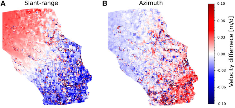
FIGURE 10. Differences between velocities measured with LabSAR and EFIDIR approach (A) along slant-range direction and (B) along azimuth direction in m/day.

6.3 Influence of the central point altitude

The previous analysis raises a question: what is the impact of the altitude of the central point chosen to build the LabSAR grid?

To answer this question, the velocity over stable ground computed with the LabSAR approach is evaluated for different central point altitudes, which vary from 0 to 4,000 m. The stable areas used for this evaluation are represented in Figure 2. They are selected to be at an altitude which range from 1,500 to 2,000 m, and have an average altitude of 1,877 m.

Figure 11 highlights that the RMSE, ME, and std for each central point altitude are roughly similar for azimuth velocities. However, the three criteria overcome a stronger variation for slant-range velocities. They all reach a minimum around 2,000 m, which corresponds to the mean altitude of the stable ground areas and are mostly symmetric, meaning that the absolute difference between the altitude of the considered pixels and the altitude of the reference point drives the error. Since the errors increase more strongly to the edge of the interval, Figure 11 suggests that the uncertainty can be considered as constant in an interval between −1,000 m and +1,000 m of the altitude of the reference point. For example, the RMSE over stable ground of the velocity magnitude range between 0.056 and 0.06 m/day for the altitude between 1,000 and 3,000 m. This highlights the need to select a central point with an altitude roughly corresponding to the median altitude of the study area.

FIGURE 11

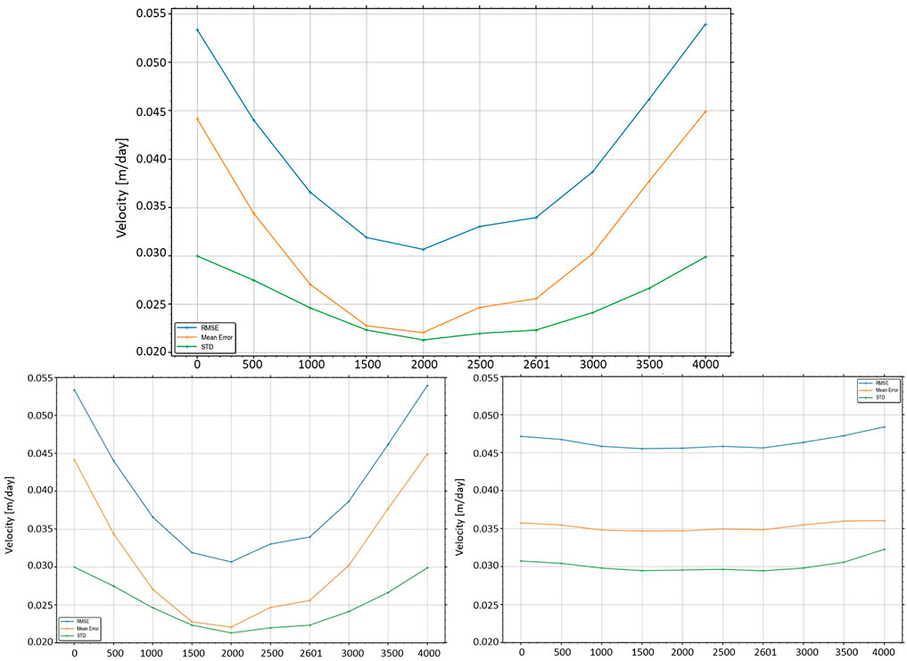
FIGURE 11. Evolution of the RMSE (in blue), mean error (in orange), and std (in green) of the velocity over stable ground for different central point altitudes used to build the LabSAR grid. The upper panel corresponds to the displacement magnitude, the bottom left panel is for the slant-range direction, and the bottom right panel is the azimuth direction.

7 Conclusion

LabSAR provides a coregistration approach based on a single GCP and satellite orbital information. It coregistrates images by using a geographical grid representing the location of the main SAR image’s pixels. This grid is spherical and defined by the geographic position of the central pixel and the SAR sampling parameters. By doing a spherical approximation, no DEM is required, and by staying in the SAR image domain, there is no deformation of the speckle statistics that arises from a coregistration on a regular grid in a geographical coordinate system (when SAR images are orthorectified for instance).

From this coregistration, multiple SAR image processing techniques can be used. In order to test LabSAR coregistation approach, we compared:

• the amplitude images obtained after coregistration with LabSAR and SNAP, in order to test the capacity of LabSAR to be used in change detection applications;

• the interferograms obtained after coregistration with LabSAR and SNAP, in order to test the capacity of LabSAR to be used in interferometric applications such as height retrieval or DInSAR;

• the displacements obtained by using EFIDIR offset tracking on LabSAR-coregistered images or by using the full EFIDIR displacement measurement pipeline.

The comparison on the amplitude of point-like scatterers showed that LabSAR coregistration has a subpixel precision. This was confirmed by the interferograms, which exhibit a high coherence and clear fringes, as well as by the displacement estimation on stable areas that shows no bias.

The comparison of the estimated phase to a phase of reference constructed from the altitude derived from the projection of the IGN RGE-Alti DEM in the image showed that the dispersion of the phase was smaller with LabSAR than with SNAP, certainly due to the less noisy fringes. In order to confirm that there was no augmentation of the phase dispersion due to an incorrect orbital fringe removal, both for LabSAR and SNAP, we computed the interferogram without this step, and added orbital fringes to the topographical fringes computed previously for the comparison. The phase difference histograms showed the same dispersion with and without this step.

Finally, the displacement estimation using LabSAR coregistration was compared to the full EFIDIR pipeline. Contrary to LabSAR, EFIDIR uses a DEM in order, first, to estimate a rough coregistration before offset tracking and then, to remove stereoscopic effects from the displacement measurement. By estimating the displacements over stable areas and verifying the temporal closure of a glacier displacement field, it was shown that both approaches have the same uncertainties. Then errors of the displacements computed on LabSAR-coregistered image were estimated by comparing the displacement at the pixel level. This comparison showed that the displacements computed on LabSAR-coregistered images are biased depending on the difference between the altitude of the considered pixel and the altitude of the reference point. This bias is mostly observed in range. By computing the displacement over stable areas for different altitudes of the reference point, we showed that the difference in altitude between the pixels and the reference point did not impact the uncertainty of the displacement measurement on an interval of −1,000 m and +1,000 m around true elevation. Hence, the reference point can be chosen in the middle of the altitude range, even if this point does not correspond to any physical point of the area.

Because LabSAR is a coregistration tool, which requires only 1 GCP and preserves the phase, it can be used for different applications in cold regions: InSAR measurement of the permafrost warming effects, snow cover mapping with SAR images, or glacier displacement measurement.

Data availability statement

The PAZ images were obtained from the Spanish Instituto Nacional de Tecnica Aerospacial (INTA) through Project number AO-001-051. Their acess is limited to the participants of the project. Requests to access the datasets should be directed to emmanuel.trouve@univ-smb.fr.

Author contributions

FW and LC: research development, data processing, result analysis, and article writing; CT: data processing and result analysis; J-MN: research development of LabSAR toolbox, data processing, and result analysis; ET: research development of EFIDIR toolbox, result analysis, and article proofreading.

Acknowledgments

The authors acknowledge the Spanish Instituto Nacional de Tecnica Aerospacial (INTA) for the PAZ images (Project AO-001-051).

Conflict of interest

The authors declare that the research was conducted in the absence of any commercial or financial relationships that could be construed as a potential conflict of interest.

Publisher’s note

All claims expressed in this article are solely those of the authors and do not necessarily represent those of their affiliated organizations, or those of the publisher, the editors, and the reviewers. Any product that may be evaluated in this article, or claim that may be made by its manufacturer, is not guaranteed or endorsed by the publisher.

References

Altena, B., and Kääb, A. (2017). enElevation change and improved velocity retrieval using orthorectified optical satellite data from different orbits. Remote Sens. 9, 300. Number: 3 Publisher: Multidisciplinary Digital Publishing Institute. doi:10.3390/rs9030300

CrossRef Full Text | Google Scholar

Altena, B., Kääb, A., and Wouters, B. (2021). Correlation dispersion as a measure to better estimate uncertainty of remotely sensed glacier displacements. Cryosphere Discuss. 16, 2285–2300. doi:10.5194/tc-16-2285-2022

CrossRef Full Text | Google Scholar

Benoit, L., Dehecq, A., Pham, H.-T., Vernier, F., Trouvé, E., Moreau, L., et al. (2015). Multi-method monitoring of glacier d’argentière dynamics. Ann. Glaciol. 56, 118–128. doi:10.3189/2015AoG70A985

CrossRef Full Text | Google Scholar

Brun, F., Berthier, E., Wagnon, P., Kääb, A., and Treichler, D. (2017). A spatially resolved estimate of High Mountain Asia glacier mass balances from 2000 to 2016. Nat. Geosci. 10, 668–673. Publisher: Nature Publishing Group.

PubMed Abstract | CrossRef Full Text | Google Scholar

Dehecq, A., Gourmelen, N., and Trouvé, E. (2015). Deriving large-scale glacier velocities from a complete satellite archive: Application to the pamir–karakoram–himalaya. Remote Sens. Environ. 162, 55–66. doi:10.1016/j.rse.2015.01.031

CrossRef Full Text | Google Scholar

Fallourd, R., Harant, O., Trouve, E., Nicolas, J.-M., Gay, M., Walpersdorf, A., et al. (2011). Monitoring temperate glacier displacement by multi-temporal terrasar-x images and continuous gps measurements. IEEE J. Sel. Top. Appl. Earth Obs. Remote Sens. 4, 372–386. doi:10.1109/JSTARS.2010.2096200

CrossRef Full Text | Google Scholar

Friedl, P., Seehaus, T., and Braun, M. (2021). EnglishGlobal time series and temporal mosaics of glacier surface velocities derived from Sentinel-1 data. Earth Syst. Sci. Data 13, 4653–4675. Publisher: Copernicus GmbH. doi:10.5194/essd-13-4653-2021

CrossRef Full Text | Google Scholar

Gardner, A. S., Moholdt, G., Scambos, T., Fahnstock, M., Ligtenberg, S., van den Broeke, M., et al. (2018). Increased West Antarctic and unchanged East Antarctic ice discharge over the last 7 years. Cryosphere 12, 521–547. doi:10.5194/tc-12-521-2018

CrossRef Full Text | Google Scholar

Gourmelen, N., Kim, S., Shepherd, A., Park, J., Sundal, A., Björnsson, H., et al. (2011). Ice velocity determined using conventional and multiple-aperture insar. Earth Planet. Sci. Lett. 307, 156–160. doi:10.1016/j.epsl.2011.04.026

CrossRef Full Text | Google Scholar

Kanti, V., and Mardia, P. E. J. (1999). Directional statistics. New York, NY: John Wiley & Sons. doi:10.1002/9780470316979

CrossRef Full Text | Google Scholar

Leclercq, P. W., Kääb, A., and Altena, B. (2021). enBrief Communication: Detection of glacier surge activity using cloud computing of Sentinel-1 radar data, preprint, Glaciers/Remote Sens. 15 (10), 4901–4907. doi:10.5194/tc-2021-89

CrossRef Full Text | Google Scholar

Leinss, S., and Bernhard, P. (2021). Tandem-x: Deriving insar height changes and velocity dynamics of great aletsch glacier. IEEE J. Sel. Top. Appl. Earth Obs. Remote Sens. 14, 4798–4815. doi:10.1109/jstars.2021.3078084

CrossRef Full Text | Google Scholar

Millan, R., Mouginot, J., Rabatel, A., Jeong, S., Cusicanqui, D., Derkacheva, A., et al. (2019). enMapping surface flow velocity of glaciers at regional scale using a multiple sensors approach. Remote Sens. 11, 2498. Number: 21 Publisher: Multidisciplinary Digital Publishing Institute. doi:10.3390/rs11212498

CrossRef Full Text | Google Scholar

Nagler, T., Rott, H., Hetzenecker, M., Wuite, J., and Potin, P. (2015). enThe sentinel-1 mission: New opportunities for ice sheet observations. Remote Sens. 7, 9371–9389. Number: 7 Publisher: Multidisciplinary Digital Publishing Institute. doi:10.3390/rs70709371

CrossRef Full Text | Google Scholar

Nicolas, J.-M., Trouvé, E., Fallourd, R., Vernier, F., Tupin, F., Harant, O., et al. (2012). “A first comparison of cosmo-skymed and terrasar-x data over chamonix mont-blanc test-site,” in 2012 IEEE International Geoscience and Remote Sensing Symposium, Munich, Germany, 22-27 July 2012, 5586–5589. doi:10.1109/IGARSS.2012.6352053

CrossRef Full Text | Google Scholar

Nitti, D. O., Hanssen, R. F., Refice, A., Bovenga, F., Milillo, G., and Nutricato, R. (2008). “Evaluation of DEM-assisted SAR coregistration,” in Image and signal processing for Remote sensing XIV. Editors L. Bruzzone, C. Notarnicola, and F. Posa (Cardiff, Wales: International Society for Optics and Photonics), 7109, 353–366. doi:10.1117/12.802767

CrossRef Full Text | Google Scholar

Petillot, I., Trouvé, E., Bolon, P., Julea, A., Yan, Y., Gay, M., et al. (2010). Radar-coding and geocoding lookup tables for the fusion of gis and sar data in mountain areas. IEEE Geosci. Remote Sens. Lett. 7, 309–313. doi:10.1109/LGRS.2009.2034118

CrossRef Full Text | Google Scholar

Plyer, A., Colin-Koeniguer, E., and Weissgerber, F. (2015). A new coregistration algorithm for recent applications on urban sar images. IEEE Geosci. Remote Sens. Lett. 12, 2198–2202. doi:10.1109/LGRS.2015.2455071

CrossRef Full Text | Google Scholar

Ponton, F., Trouvé, E., Gay, M., Walpersdorf, A., Fallourd, R., Nicolas, J.-M., et al. (2014). Observation of the argentière glacier flow variability from 2009 to 2011 by terrasar-x and gps displacement measurements. IEEE J. Sel. Top. Appl. Earth Obs. Remote Sens. 7, 3274–3284. doi:10.1109/JSTARS.2014.2349004

CrossRef Full Text | Google Scholar

Scheiber, R., and Moreira, A. (2000). Coregistration of interferometric sar images using spectral diversity. IEEE Trans. Geosci. Remote Sens. 38, 2179–2191. doi:10.1109/36.868876

CrossRef Full Text | Google Scholar

Scher, C., Steiner, N. C., and McDonald, K. C. (2021). EnglishMapping seasonal glacier melt across the Hindu Kush Himalaya with time series synthetic aperture radar (SAR). Cryosphere 15, 4465–4482. Publisher: Copernicus GmbH. doi:10.5194/tc-15-4465-2021

CrossRef Full Text | Google Scholar

Vernier, F., Fallourd, R., Friedt, J. M., Yan, Y., Trouvé, E., Nicolas, J.-M., et al. (2011). Fast correlation technique for glacier flow monitoring by digital camera and space-borne sar images. J. Image Video Proc. 2011, 11. doi:10.1186/1687-5281-2011-11

CrossRef Full Text | Google Scholar

Wegmuller, U., Werner, C., and Strozzi, T. (1998). “SAR interferometric and differential interferometric processing chain,” in IGARSS '98. Sensing and Managing the Environment. 1998 IEEE International Geoscience and Remote Sensing. Symposium Proceedings. (Cat. No.98CH36174), Seattle, WA, USA, 06-10 July 1998, 1106–1108. doi:10.1109/IGARSS.1998.6996872

CrossRef Full Text | Google Scholar