
95% of researchers rate our articles as excellent or good
Learn more about the work of our research integrity team to safeguard the quality of each article we publish.
Find out more
ORIGINAL RESEARCH article
Front. Remote Sens. , 30 June 2022
Sec. Remote Sensing Time Series Analysis
Volume 3 - 2022 | https://doi.org/10.3389/frsen.2022.930021
 Suvrat Kaushik1,2*
 Bastien Cerino2
 Emmanuel Trouve2
 Fatima Karbou3
 Yajing Yan2Ludovic Ravanel1,4Florence Magnin1
This paper investigates the backscatter evolution and surface changes of ice aprons (IAs) by exploiting time series of X- and C-band SAR images from PAZ and Sentinel-1 satellites. IAs are extremely small ice bodies of irregular shape present on steep slopes and complex topographies in all the major high-Alpine environments of the world. Due to their small size and locations in complex topographies, they have been very poorly studied, and very limited information is known about their evolution and responses to climate change. SAR datasets can provide handy information about the seasonal behaviour of IAs since physical changes of IA surfaces modify the backscattering of RaDAR waves. The analysis of the temporal variations of the backscatter coefficient illustrates the effects of increasing temperatures on the surface of the IAs. All IAs considered in the analysis show a strong decrease in backscatter coefficient values in the summer months. The backscattering patterns are also supported by the annual evolution of the coefficient of variation, which is an appropriate indicator to evaluate the heterogeneity of the surface. Higher mean backscatter values in the X-band than in the C-band indicate surface scattering phenomena dominate the IAs. These features could provide key information for classifying IAs using SAR images in future research.
Satellite remote sensing is an attractive alternative to costly and time-consuming field observations (Gao and Liu 2001) and has shown great potential in a variety of applications for mountain environments, such as glacial hazards monitoring (Bühler et al., 2013; Nefeslioglu et al., 2013), geomorphological mapping (Loibl and Lehmkuhl, 2013; Kääb et al., 2014; Meier et al., 2018), climate change impact assessment (Rafiq and Mishra, 2016; Kraaijenbrink et al., 2017; Magnin et al., 2019; Rastner et al., 2019) and glacier dynamics (Strozzi et al., 2002; Sam et al., 2018; Farinotti et al., 2019). Different satellite data types like optical (Luckman et al., 2007; Berthier et al., 2014), SAR (Rabus and Fatland, 2000; Quincey et al., 2009; Waechter et al., 2015), altimetry (Kaab, 2008; Neckel et al., 2014; Trantow and Herzfeld, 2016) and derived products like Digital Elevation Models (DEMs) (Rignot, 2003; Bamber and Rivera, 2007) are used for mountain studies. All data types have their advantages and limitations, and the choice of data depends on the application (e.g. terrain complexity of the study region, research objective) and the data availability. Optical/multispectral remote sensing is the oldest and most used monitoring technique for snow-covered regions, with a well-established history (König et al., 2001; Dietz et al., 2012). SAR sensors allow for all-day and all-weather observations, which is particularly important for observations in polar or high mountain regions that experience polar darkness in winter and heavy cloud cover conditions (Robinson et al., 1984; Lubin and Massom, 2005). In addition, the ability of electromagnetic waves to penetrate the snowpack and interact with surface and subsurface features is a significant advantage of SAR imagery over optical imagery. In the case of snow/ice studies, the SAR signal with longer wavelengths can penetrate deeper into the snowpack and provide valuable information about snowpack characteristics like the snow grain size, the snow depth and the amount of liquid water in the form of snow water equivalent (SWE) (Floricioiu and Rott 2001). Using the potential of SAR, many successful studies have been published for various applications in glacier and snow/ice studies: snow cover mapping (Sokol et al., 2003; Thakur et al., 2013), snow depth retrieval (Awasthi et al., 2017; Li et al., 2017), SWE estimation of the snowpack (Patil et al., 2020), glacier zones delineation (Arigony-Neto et al., 2007; Kundu and Chakraborty, 2015; Fu et al., 2020) and snow/ice classification (Moen et al., 2015; Casey and Haas, 2016; Khaleghian et al., 2021).
Considering the number and often recentness of these applications, we can safely state that SAR remote sensing techniques have evolved rapidly in recent years. However, challenges remain in imaging areas of high relief and complex topographies (Taylor et al., 2021) because the side-looking geometry of SAR acquisitions results in slant range and slope dependent cell resolutions. The SAR acquisition geometry also results in well-known geometric distortions, which become more severe as the complexity of terrain surfaces increases (Gelautz et al., 1998; Chen et al., 2018). In addition, since the backscattered signal of each pixel of SAR imagery is the coherent sum of the backscattered signals from all the scatterers (ground features that reflect RaDAR waves) in the imaged area, the resulting speckle degrades the final image quality (Lucas, 1995; Chan and Peng, 2003). Moreover, a critical element for SAR processing, DEMs also suffer from increasing inconsistencies in steep slopes. Therefore, although SAR images have seen numerous applications in mountain areas, they have mainly been limited to large and low slope angle glaciers (generally <15°) (Joughin et al., 2010). Small ice bodies on steep rock slopes like hanging glaciers, snow and ice covers, snow-filled couloirs, glacierets and ice aprons often exist in cirques or niches in rock walls or steep rock faces, making their global observation extremely challenging (Helfricht et al., 2015). As a result, these ice features have rarely been studied. In situ observations are also limited; hence there exists a critical gap in understanding these features.
Guillet and Ravanel, 2020 state that ice aprons are very small (typically smaller than 0.1 km2) ice bodies of irregular outline that lie on steep slopes >40° that may not be thick enough to deform under their own weight. Guillet et al., 2021 showed that IAs constitute a critical component of the mountain ecosystem because of the old age of the ice they preserve, but very few studies have been dedicated to understanding their characteristics. Most glacier inventories fail to consider IAs as a specific glacial entity and often show them as part of larger glacial systems (Benn and Evans, 2010). This results from our lack of understanding of differentiating these small features from other glacier parts. The small size and the complex topography associated with the locations of the IAs also prevent previous studies from attempting to understand their physical behaviour using SAR images. As a result, our understanding of the behaviour and geometric changes of these small ice bodies is very limited.
Keeping this perspective, this paper aims to understand the physical behaviour of IAs in the Mont-Blanc massif (MBM hereafter) (western European Alps), using time series of X-band PAZ and C-band Sentinel-1 images. For this, we made a first regional synthesis of the temporal changes occurring at the surface and sub-surface of the IAs through the annual cycle. Further, we attempted to link the temporal changes in SAR backscattering response to the annual meteorological changes. We also tried to understand the behaviour of the IAs in different RaDAR wavelengths of SAR images for a better understanding of the scattering characteristics of the IAs.
The paper is organized as follows: Section 2 provides the background theory on the interactions of the RaDAR waves with snow/ice and glacier surfaces, Section 3 presents the study area and the datasets used for the study, Section 4 describes the methodology and the processing steps, Section 5 deals with analyzing the results followed by a brief discussion to interpret the results and Section 6 summarizes the primary research outcomes from the study in the form of conclusions.
SAR imaging works on the principle of active imaging, i.e., the satellite sensor transmits electromagnetic (EM) radiation with varying wavelengths between 0.3 and 0.01 m and receives the returned echoes (called backscatter) from the Earth’s surface (Wiley, 1985; Bruder, 2013). The backscattering from the ground surface essentially depends upon the dielectric constant of the surface and medium, the surface roughness, and the shape and size of the scatterers (Stiles and Ulaby, 1980). If the target surface has a layer of snow, the longer lengths of the EM wave can penetrate the snowpack up to depths of tens of meters. In this case, the final backscattered signal received by the SAR sensor is the sum of the contributions from within the snowpack and the underlying ground/rock. The backscattered signal received from the snowpack is the sum of the surface scattering at the air/snow interface, volume scattering from inside the snowpack, scattering at the rock/snow interface and volume scattering from the ground surface beneath (in case the penetration depth of the SAR signals is high enough). Many mathematical models based on physical and empirical laws have been formulated to model the backscattering response from the snowpack (Cooper, 2007). SAR backscattering signals from snow/ice depend on (1) sensor parameters such as the wavelength of the signal, the polarization (single pol (HH, VV), dual-pol (HH/HV or VV/VH) or quad/full pol (HH/VV/HV/VH) and the incidence angle; and (2) snowpack or ground characteristics, which include the density, the liquid water content, the size and shape of the particles and the surface roughness. In general, longer wavelengths penetrate the snowpack deeper and thus produce more volume scattering (Johansson et al., 2018). X-band SAR (2.4–3.75 cm, 8.0–12.5 GHz) is more sensitive to the snowpack than both the L (23.5 cm, 1–2 GHz) and C-band (5.6 cm, 5.3 GHz) SAR. In glacier studies, the dielectric constant values play a significant role in analyzing the internal properties of the snow/ice. The dielectric properties of snow at a particular signal wavelength are dependent on the relative proportion of liquid and solid water. Studies by Brown et al., 1999 and Casey and Haas, 2016 have shown that even a small amount of liquid water (∼3–5% liquid water content) can drastically affect the penetration depths of EM signals in snow/ice. For example, C-band SAR can potentially penetrate up to a depth of around 10 m in dry snow (Mätzler, 1987), but as the snowpack begins to melt, the dielectric properties of the snow change considerably, and the penetration depth is reduced to as low as 3 cm (Ashcraft and Long, 2006; Zhou and Zheng, 2017).
Longer L-band (23.5 cm, 1–2 GHz) wavelengths penetrate 5–10 m deeper than C-band into the snowpack and travel almost unaffected through dry snow. Thus, studies involving the L-band to analyze snow cover properties are rare because they provide significantly less information about the properties of the snow (Strozzi et al., 1997).
The snowpack properties like snow grain size, density, roughness, stratigraphy, and water content in different snow zones are different. As a result, the RaDAR scattering characteristics, represented as backscattering coefficient values, should also be different. This contrast in backscattering strength helps delineate different snow zones from SAR image data (Ramage et al., 2000; Zhou and Zheng 2017; Winsvold et al., 2018). A different approach to classifying snow zones is based on the glacier zones more familiar to glaciologists. For the study area, we considered the local Equilibrium Line Altitude (ELA) at an altitude of 3,300 m a.s.l. based on the analysis of Rabatel et al., 2013. Areas below this altitude range fall in the ablation zone of a glacier system, as ablation rates are generally higher than accumulation rates in the MBM region. Areas above the ELA are said to be the glacier’s accumulation zone. Regions around the ELA are said to be the transition zone of the glacier system, where ELA can vary from 1 year to the next depending on the meteorological conditions.
The glacier system can accordingly be divided then into three commonly known glacier areas, namely, the ablation zone (below the ELA, i.e., < 3,300 m a.s.l.), the transition zone (the zone around which ELA fluctuates each year, i.e., 3200–3400 m a.s.l.) and the accumulation zone (regions above the ELA, > 3,400 m a.s.l.). We add a fourth zone to this standard classification criterion called the IA zone, a separate, steeper entity above the accumulation area (Figure 1). Figure 2 shows the profile along the Brenva glacier (on the Italian side of the MBM) on a mean image created by stacking 28 PAZ descending images.
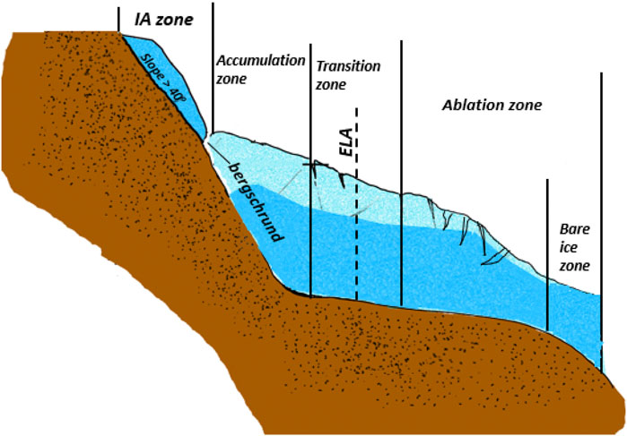
FIGURE 1. Glacier zones. Brown: bedrock, dark blue: ice, light blue: snow.

FIGURE 2. Temporal mean of 28 PAZ descending images acquired in 2020. Glacier profile along the Brenva glacier on the Italian side of Mont-Blanc massif (MBM) (red). The image shown is in the original RaDAR geometry.
Since the snowpack properties are also profoundly affected by the meteorological parameters, these variations differ across seasons of the year. Hence, the temporal backscatter response of RaDAR waves across different glacier zones is discussed in the following paragraphs.
Due to intense melting at the lowest elevations, especially at the glacier front, bare ice is usually exposed as the firn cover has ablated away. A smooth bare ice surface either absorbs RaDAR signals if it penetrates the ice pack or reflects the waves away from the sensor because they act as a specular surface, especially when meltwater is present on the ice surface. As a result, the glacier fronts typically show very weak backscattering, especially in the summer months. Surface melting is also intensive; hence, the snowpack is damp, most noticeably during the spring (associated with frequent rainfall events at lower elevations) and summer months. As a result, the penetration depth of the RaDAR wave decreases dramatically, and the backscattered signal is the lowest. In fall and winter, however, the meltwater starts refreezing with the onset of the temperature drop. According to Marsh et al., 2021, alternating sessions of melting and refreezing can produce large snow grains due to the metamorphism that acts as effective scatterers and the overall backscattering increases. After the summer and before winter, the fall period defines when the meltwater starts to refreeze again, forming large ice crystals. This can lead to an increase in the backscattering intensity in the images analyzed after the summer period.
This is the glacier system’s most dynamic (with the most variations) zone. It experiences seasonal changes throughout the year. In summer, occasional and frequent surface melting dominates. The meltwater can either percolate down and spread into layers or stay on the surface and make the snowpack surface damp. If the meltwater percolates and later recrystallizes, it can form large ice pipes and lense, profoundly affecting the SAR signal of long wavelengths. In this frozen state, the ice layers backscatter RaDAR waves strongly, and we notice a sharp rise in the RaDAR backscattering signal, especially in images acquired in fall and winter. On the contrary, if the meltwater stays on the surface, making the snow damp, it can lead to a sharp signal drop, as observed in the wet snow zone. The dynamics of the transition zone change with the meteorological parameters and the regional ELA shifts within the zone.
As we move higher along the glacier system, the effects of meteorological changes become less significant. The accumulation zone of the glacier system is mainly defined by the presence of dry snow for a large part of the year. The most dominant scattering mechanisms for dry snow are volume scattering from the snowpack and surface scattering from the snow/ice interface. Since the thickness of the snowpack in glaciers is generally substantial (more than the penetration depth of X-band RaDAR), the RaDAR waves do not reach the rock surface. Hence, for shorter wavelengths, volume scattering from within the snowpack dominates.
Previous studies by Jezek et al., 1993; Partington, 1998, and Rau and Braun, 2002 have suggested that this zone appears very dark with low backscattering values, especially at longer wavelengths. However, exceptions are observed in regions where snow accumulation is low, and snow crystals can grow near the surface (Liu et al., 2006). Also, with smaller wavelengths like the X-band, where the surface scattering phenomenon plays an essential role, the high backscatter values are related to wind action and depth-hoar development because of internal temperature and moisture gradients (King et al., 2015). The snow grain size is generally uniform, but frequent dry snow events and heavy winds increase surface roughness, which leads to an increase in RaDAR backscattering at smaller wavelengths like the X-band. Due to the low penetration depth of the X-band, volume scattering from layers close to the surface and surface scattering dominate.
The last zone in focus is the IA zone, which has not yet been studied or classified separately from the other glacier zones before this study. IAs occur at the highest part of the glacial system (Figure 1) and occupy the steep headwalls of cirque and slope glaciers. They usually occur on very steep slopes (>40°), where fresh snow accumulation is limited because of the steepness of the surface (Magnin et al., 2017). IAs, as the name suggests, are thin (thickness up to a few meters for most regions), cold (temperature <0°C) ice bodies that may not be thick enough to deform under their own weight (Guillet and Ravanel, 2020). The backscattering mechanism of the snow/ice pack depends on the complex multi-layered structure, the grain size, the density, the depth, the number of impurities, the stratigraphy, and the surface roughness. Since the physical characteristics of IAs are different from other types of glaciers, we expect their resulting backscattering response to time series also to be different.
Since IAs are present on very steep slopes, so even in winter months, IAs are generally covered by only a thin layer of fresh dry snow (in the order of a few decimeters). Below this thin layer of snow is a highly metamorphosed, rigid and solid stratified layer of ice that extends to the base of the IAs (Guillet et al., 2021).
As a result, the backscattered signal by an IA in winter comes from the snow/ice interface, which creates a dielectric discontinuity for the RaDAR signal by the difference in the electrical properties of ice crystals and dry snow. In summer, the dielectric discontinuity is created by the layer of water, wet snow, mixed with dry snow in parts and the ice layer. Since these discontinuities occur at shallow depths or the surface of the IA, surface scattering or shallow sub-surface volume scattering mechanisms dominate. However, as the snow becomes wet, the surface scattering at the air/snow interface dominates (Thakur et al., 2013; Guneriussen, 1997). Further in this study, we analyze the temporal backscattering response of IAs in the following sections utilizing both X- and C-band RaDAR datasets.
The study area is the MBM (Figure 3), located in the north-western Alps. Its total area of ∼550 km2 is shared by three countries: France, Italy and Switzerland. It is the highest and most glacierized massif in the French Alps, with around 20% of its total area covered by glaciers (Berthier et al., 2016). The largest glacier in the MBM is the Mer de Glace, with an overall total area of 30 km2. The massif consists of 12 large glaciers broader than 5 km2, bordered by steep walls (Gardent et al., 2014). Deep valleys on the sides of the MBM are mainly built-in highly fractured rocks. The steep, irregular terrain combined with events of glacial erosion promotes the development of slope glaciers and smaller ice bodies like IAs. Considering the high average elevation of the massif, IAs and large glacier accumulation zones lie above the regional ELA. The geological setting of the MBM also promotes the development and existence of permafrost at high elevations. Modelled analysis by Magnin et al., 2015 shows that out of the total 85 km2 of steep slopes (>40o) on the French side of the MBM, almost certainly, about 45–79% of the area would be underlain by permafrost at elevations above 1900 m a.s.l. in N faces and above 2,600 m in S faces where structural settings are favourable. Permafrost would be more continuous above 2,600 m. Above 3,600 m, permafrost would most certainly occupy the entirety of the steep rock walls irrespective of the aspect. These factors make MBM the perfect study site for an in-depth study of the high mountain steep slope ice bodies like IAs. Figure 3 shows the locations of the 19 IAs (in red) considered for analysis in this paper. The yellow line on the Brenva glacier (the Italian side of the MBM) shows the glacier profile from the ablation zone to the IA zone.
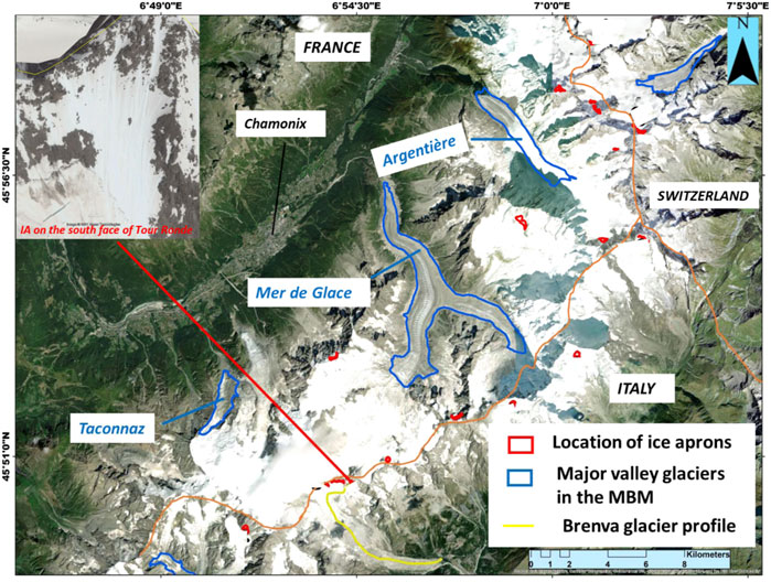
FIGURE 3. The study area, Mont-Blanc massif. The base image shown is taken from ArcGIS World Imagery database.
The datasets used for analyzing the temporal behaviour of IAs on RaDAR images are described in detail in this section. Table 1 provides all datasets used for the study and their characteristics.
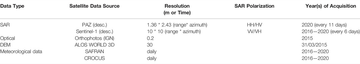
TABLE 1. Datasets used for the study.
This study analyses a time series of high-resolution PAZ images and a time series of medium resolution Sentinel-1 images. Data from both satellites have been selected with similar orbit characteristics to maintain consistency in our comparison. We processed 28 Single Look Complex (SLC) PAZ descending images available in 2020. All images of PAZ are dual-polarization (HH/HV) acquired at 5 h 44 am over the study area in descending orbits with an incidence angle of 37.8° and every 11 days from 12/02/2020 to 25/12/2020. 244 Ground Range Detected (GRDH) Sentinel-1 A/B images in descending orbits, covering the period from 2016 until 2020, were downloaded and processed. The nominal incidence angle for Sentinel-1 images is 38.3o. These images are acquired at 05 h 35 am every 6 days. Images from both satellites cover almost the whole study region, allowing the selection of different areas spread across the massif with different topographic characteristics.
The backscattering change observed in SAR time series needs to be interpreted from other data. Meteorological data, in particular the air temperature and the total precipitation, are the essential parameters that influence the physical state of the snowpack. Additional information like the total water content of the snow and snow depth can also help better understand the results obtained from the SAR time series. Therefore, we utilized the SAFRAN reanalysis datasets (Durand et al., 1983, 2009), which provide temperature, precipitation, wind speed, and other meteorological variables at an hourly time step. This dataset is available as NetCDF files from 1958 for all the French massifs. Each meteorological variable is available at every 300-m-elevation band, at 0, 20, 40°s slopes and eight aspects. Snow depth and snow liquid water content simulations are taken from Crocus reanalyses detailed snow cover model (Brun et al., 1989). Crocus is coupled with the ISBA land surface model within the SURFEX (EXternalized SURFace) simulation platform (Masson et al., 2013).
Aerial orthophographs at 20 cm resolution, downloaded from Geoportail IGN (Institut national de l’information géographique et forestière), were used as reference images for validation. The DEM used for processing the SAR images was ALOS WORLD 3D (AW3D30) provided by JAXA (Japanese Aerospace Exploration Agency) at 30 m resolution. According to Tadono et al. (2016), the vertical and horizontal accuracy of the DEM is better than 5 m. The choice of the DEM was based on the quality and the availability over the entire study region.
To compare the behaviour of the IAs with other glacier regions and differentiate them as unique glacier entities, we processed two large time series of SAR images from X-band PAZ in 2020 and C-band Sentinel-1 from 2016 to 2020. The temporal profiles of backscattering coefficients and statistical parameters are extracted after coregistration and calibration to avoid the effects of geometric distortions or artefacts that commonly plague SAR images. The flowchart of the processing chain performed is given in Figure 4. Detailed explanations for some key steps are given in subsections 4.1–4.5. After this processing chain, temporal profiles of backscattering signals are analyzed for 19 visible IAs in the PAZ images and 8 IAs visible in both Sentinel-1 and PAZ images. Besides the analysis of the temporal profiles of the backscattering signal, we also compute the coefficient of variation (CV) to assess the surface homogeneity of IAs. Meteorological variables such as air temperature, precipitation, and liquid water content are also deployed for a joint analysis with the temporal profiles of backscattered signals.
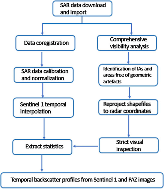
FIGURE 4. Flowchart of the processing steps.
IAs are very small ice bodies located on very steep slopes. The slant range acquisition geometry of SAR images is always associated with geometric distortions, which can create geometrical artefacts (GA): strong foreshortening, layover (active and passive) and shadow (active and passive) (Kaushik et al., 2021a). To study the temporal evolution of backscattering response from IAs, it is necessary to find areas free from these artefacts. An extensive visibility analysis was performed to build a mask that incorporates all kinds of GAs for identifying and selecting clean (referred to as ‘visible’) IAs for further analysis. For this, we follow the methodology proposed by Cigna et al., 2014, which combines the results from the R-Index (RI) (Notti et al., 2010) and layover-shadow simulations using ray-tracing algorithms (Kropatsch and Strobl, 1990). The RI, which effectively integrates local topography and satellite acquisition parameters, can only identify areas of active layover and foreshortening regions. Passive layover and active and passive shadow regions thus need to be mapped using ray-tracing algorithms. A final mask that incorporates all kinds of GAs can thus be prepared by combining the results from the two methods. Using this GA mask as a base, we carefully select our observation areas, avoiding regions affected by GAs. Moreover, we only selected regions of interest with more than 100 pixels to obtain reliable estimates of statistical parameters. A detailed analysis of this method could be found in Kaushik et al., 2021b.
The SAR SLC images were downloaded and imported into SARScape (L3Harris Geospatial, 2022) for basic pre-processing required to compute the image time series. All images were accurately coregistered at sub-pixel pixel accuracy to remove the bias from spatial shifts between repeat pass acquisitions. After this, the coregistered datasets were radiometrically calibrated and normalized. Radiometric calibration is vital when comparing RaDAR data from different sensors, in different acquisition modes, at different periods or generated by different processing algorithms. Radiometrically calibrated SAR images represent the backscattering coefficient, corresponding to the transmitted and backscattered power ratio. It is a dimensionless quantity, represented either in the linear scale or by log normalizing the linear values (10* log10 of the linear values) in the dB scale. Radiometric calibration depends on SAR sensor-related parameters, usually available in the metadata and on the geometry factors dependent on the local topography. At the calibration step, we used SARScape to correct for two effects: (1) the different incidence angles of the satellites, which affect the backscattering signal and (2) the influence of the topographic factors like terrain slope. ALOS World 3D DEM was used as a reference to determine all the terrain parameters correctly. Radiometric normalization was applied to all images to correct for the dependency of backscatter on the difference in incidence angles between acquisitions. This is also particularly important for wide swath datasets like Sentinel-1, where incidence angles change from near range to far range. We applied the most used square cosine correction technique given by Leberl (1984). After the calibration and normalization, the final product gives the value of the backscattering coefficient, which is the RaDAR backscatter per unit area, commonly called sigma nought (denoted as sigma0), expressed in decibel (dB). All values used in our comparison and analysis are expressed in sigma0.
To compare the X- and C-band’s backscattering, we use the data from 2020 as PAZ data are available only for this period. For a fair comparison, it is necessary to compare images acquired in the same configuration (e.g., geometry, polarization) and cover the same period with acquisitions at as close as possible hours and dates. The latter conditions are significant for mountain terrains where weather changes can be significant and very quick. If the temporal sampling frequency difference between the two sets of images is not considered, the significant difference can introduce uncertainties that are hard to quantify (Loew et al., 2017). However, the PAZ data are acquired every 11 days, while the Sentinel-1 data are available every 6 days; it is impossible to have both data acquired in the same configuration for the same dates. Since co-polarized images from HH and VV polarizations usually provide similar backscattering coefficients (Lubin and Massom, 2005), we can compare HH polarized images from PAZ with the VV polarized images from Sentinel-1. The incidence angles of both datasets are similar, and all images have been radiometrically calibrated and normalized, so the effect of the difference in incidence angle is negligible. Therefore, our main focus was to reduce the impact of different time sampling frequencies. Various approaches to linear interpolation can overcome this problem by resampling Sentinel-1 images for 2020.
For this analysis, since Sentinel-1 images are available at a regular and higher temporal sampling frequency (61 images every 6 days for the entire year of 2020) compared to PAZ, we chose to resample Sentinel-1 time series at the PAZ acquisition dates. The temporal signal at each pixel location is over-sampled in the frequency domain using a Discrete Fast Fourier transform (D-FFT) and zero-padding to obtain a daily sampling of the temporal profile after the inverse Fourier Transform. The values of the dates where PAZ images are then available (almost every 11-days) are kept to build the interpolated Sentinel-1 image time series at the exact dates as the PAZ image time series.
For the temporal profile analysis along with the glacier profile, the PAZ images from 2020 were divided into four seasons: Winter (December 21 - March 20), Spring (March 21 - June 20), Summer (June 21 - September 20) and Fall (September 21 - December 20). All PAZ images that fall within the seasonal range were temporally averaged to reduce the effects of speckle noise from individual images. Hence, we built a mean Summer (average of all 11-days images for June 21 - September 21) and fall, winter, and spring images. Seasonal backscattering profiles along glaciers are generated using the four seasonal mean images (winter, spring, summer and fall). The sigma0 values used in these profiles are obtained by extracting the mean value for a 9x9-pixel spatial window instead of just taking the pixel values.
To locate the visible IAs, their shapefiles, originally digitized in a GIS environment on very high resolution optical/aerial images in the WGS 84 coordinate system, were transformed in the RaDAR range/azimuth coordinate system. A rigorous visual inspection was performed to ascertain that no pixel from any type of geometric artefacts falls within the selected IA shapefiles. Then, conventional basic statistical features (mean, standard deviation, min-max values) can be computed using all pixels inside the shapefiles.
The mean (first-order) helps observe the backscattering coefficient’s temporal variation related to the snow/firn/ice. But the standard deviation (second-order) is not very useful for SAR imagery affected by multiplicative noise. To investigate homogeneity in a set of pixel values affected by speckle, a conventional feature is the so-called coefficient of variation (CV), also commonly known as relative standard deviation, defined as a ratio of the standard deviation σ by the mean value μ:
CV can be calculated spatially, for example, over a window or sub-window for speckle filtering (Nicolas et al., 2001), temporally between a time series of images (Koeniguer and Nicolas, 2020) or spatiotemporally (Lê et al., 2015) to detect changes. As a ratio, CV values should not be affected by possible radiometric calibration errors. For SLC images, the CV is expected to be close to 1 in homogenous areas with a fully developed speckle. CV values less than 1 usually indicate the presence of a permanent scatterer with a very high deterministic component, whereas values significantly larger than 1 reveal heterogeneous areas interpreted as the presence of texture. If speckle filters are used, CV values are expected to be close to 1/√ Leq where Leq is the equivalent number of looks achieved by the filter.
Here, we propose to use the spatial CV (across the entire area of the IA) to analyze the temporal evolution of the homogeneity of IAs surfaces. The estimator of CV in Equation 1 is sensitive to the number N of samples in the estimation window. To take this uncertainty into account, the statistical behaviour of the CV estimator can be modelled (Koeniguer and Nicolas, 2020), and a confidence interval derived:
In Equation 2, CVray = 1 and σray = 1, (where ray stands for the Rayleigh criteria), k is a constant value defined by the confidence level based on the standard deviations. For our analysis, we choose k = 3, N is the number of pixels in the given area. The interval defined around the CV = 1 is called the Rayleigh interval, around which the CV estimator is expected to vary. The variation of the spatial CV values within this interval would thus indicate a truly homogenous area. Any significant positive deviation from this interval indicates surface changes resulting from melting, crevasses, the appearance of a strong scatterer like rocks, etc.
The section is divided into five sub-sections which describe: 1) the seasonal variation of the X-band backscatter through the Brenva glacier system (section 5.1), 2) temporal backscatter profiles for different IAs in the MBM using X- and C-band data, and their comparison with climate variables (section 5.2), 3) variation of the spatial coefficient of variation through the year for 8 different IAs in PAZ images (section 5.3), 4) accuracy assessment for the temporal interpolation applied to Sentinel-1 images to match the dates of PAZ images (section 5.4) and 5) comparison of the backscatter coefficient in X- and C-bands for 8 IAs (section 5.5).
Figure 5 shows the evolution of the RaDAR backscatter signal along the Brenva glacier through different seasons. The glaciological understanding of this area is used to delineate different zones. Based on Rabatel et al. (2013), we placed the regional ELA line conservatively at 3,300 m a.s.l. Accordingly, the ablation zone (<3,200 m a.s.l.), the transition zone (3,200–3,400 m), the accumulation zone (3,400–3,560 m) and the IA zone (>3,560 m) were delineated.

FIGURE 5. Temporal profile of backscattering signals on PAZ images in 2020 along the Brenva glacier.
The first observation is that the sigma0 values are higher in fall and weaker in summer for almost all glacier zones, with the average values being −24,15 dB in spring and −31.38 dB in summer −21,86 dB in fall and −22.52 dB in winter. This observation is consistent with Partington (1998), Jezek (1999) and Rau and Braun (2002). Indeed, in summer, water content increases due to summer melting, which leads to a decrease of the backscattered signal, while in fall, the refreezing of water can lead to recrystallization of snow/ice, causing an increase in backscattered values.
In a large part of the ablation zone, up to an elevation of 2,900 m a.s.l., we are in the bare ice zone (as defined in Figure 1) most of the year, and the signal strength does not show strong variations. The small peaks observed in this bare ice zone result from an increased backscattering strength due to the crevasses that act as a strong scatterer, as highlighted by Forster et al. (1996), Steffen and Heinrichs (2001) and Marsh et al. (2021). As we move higher in the ablation zone, we notice an increase in backscattering signals for all seasons, especially in fall and winter. The sharp increase in signal strength observed at 3,000 m a.s.l is due to the strong layover observed in the SAR image (Figure 2).
The transition zone is characterized by a fluctuating seasonal profile defined by a sharp increase and drop in sigma0 values. The drop and increase in signal strength can be correlated with either liquid water (for a drop in signal) or recrystallized ice/snow (for an increase) on the surface, especially in the fall and winter profiles.
In the part of the accumulation zone between 3,400 and 3,570 m a.s.l., we observe a sharp rise in backscattering values with the elevation for all seasonal profiles. The four seasonal backscattering signals become closer at 3,500 m as similar backscattering trends are observed throughout the year.
The IA zone is separated from the accumulation zone by a bergschrund. The data points taken around the bergschrund show a sharp rise in backscattering values, indicating the presence of a deep fracture which causes the backscattering signals to increase (around 3,560 m a.s.l.). This increase can be a valuable indicator for detecting the bergschrund to delimit the IA zone boundaries. The observed values for the IAs zone for all profiles are comparable to that of the bare ice zone present at the glacier front. However, two different behaviours can be observed: i) the summer values are the weakest in the IA zone, whereas they can be higher in the bare ice zone due to debris and crevasses; ii) the spring values are the lowest in the bare ice zone due to the presence of wet snow at low altitudes, whereas spring and winter values are very close on the IA zone.
From the visibility analysis we performed for the descending PAZ images, we identified 19 IAs visible in the study region. Figure 6 shows the annual variation of the backscattering response for the 19 IAs, classified according to their elevation. At a first look, all IAs seem to show a very similar trend, with a noticeable drop in signal strength in summer (July and August) and a stable period before and after the summer months. The average drop in signal strength for all IAs was around 4.5 dB, which agrees with the results shown previously by Dehecq et al., 2016 who also reported a drop of 3 dB in the snow-covered areas while working with the X-band. The average minimum backscattering value was −14.5 dB, similar to the values previously reported by Phan et al., 2014 for the wet snow (working with the X-band). The onset of the melting period for all IAs is also similar, with the first major melting event observed after mid-July (which begins at the start of the summer months in the northern hemisphere). A gradual increase in the backscattering signal is observed from the first week of September, with a prolonged period of stability persisting for all IAs from October till the end of March, with meteorology not significantly influencing the backscatter.

FIGURE 6. Temporal backscattering profile for 19 visible IAs classified depending on their elevation using 28 PAZ images in 2020. Altitudes in m a.s.l.
To observe the long-term temporal evolution of backscattering values, a similar analysis was done using 244 Sentinel-1 A/B images for 4 years, from 2016 to 2020 (Figure 7). Similar trends for IAs behaviour were observed over the 4 years: a period of stability in the fall to spring months, while a noticeable drop was observed with the onset of the summer months. The average signal drop over four summers for all the IAs was ∼6.53 dB. For the highest elevation IAs, the mean drop in the summer months observed was ∼6.71 dB, while the same for middle elevation IAs was ∼6.02 dB, and for the lowest elevation, IAs were ∼6.86 dB. Considering the locations of the IAs (at very high elevations above the regional ELA), it can be concluded that liquid water exists even at the highest elevations during the summer months in the MBM. The drop in signal strength for the C-band is more than what was observed for the X-band. This difference may arise due to the different wavelengths and their subsequent interaction with the IAs surfaces. Overall, a decrease in signal strength is observed in both X- and C-bands, indicating the effects of melting on the IAs even at higher elevations.
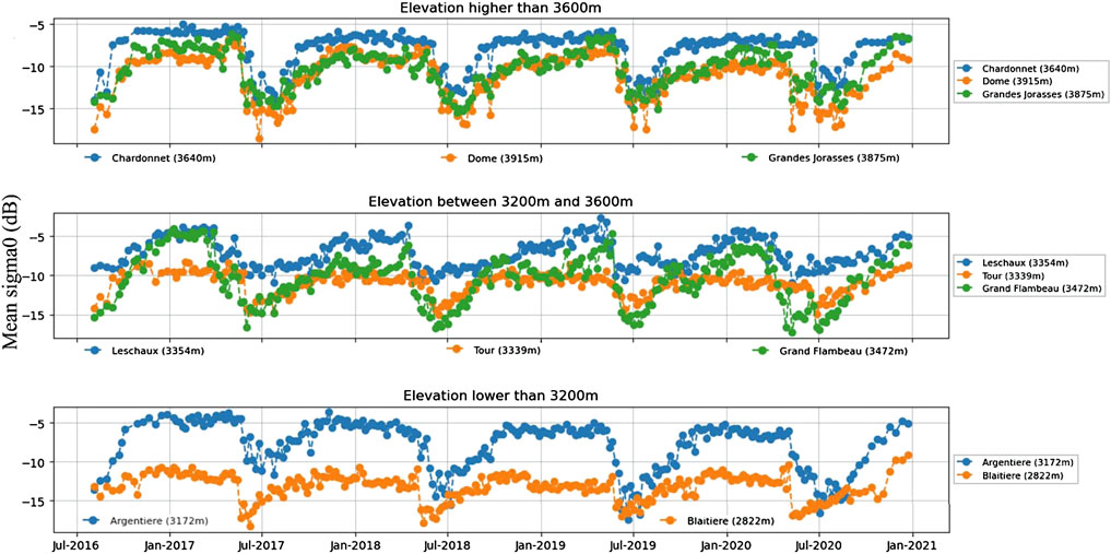
FIGURE 7. Temporal backscattering profile for 8 visible IAs using Sentinel-1 images (2016–2020).
Figure 8 shows the joint analysis of the backscattering evolution on Sentinel-1 images and meteorological variables such as air temperature, precipitation, and liquid water content for the Chardonnet IA (at 3,650 m a.s.l.). The melting signs (sudden drop in backscattering values) are observed for the Chardonet IA when the mean air temperature rises above 274 K (1°C). The drop in signal strength can be directly attributed to the melting of the IAs, and the subsequent increase of the liquid water content, which decreases the dielectric constant. The melting trend ceases as the air temperature drops to lower than 266 K, and a gradual increase in sigma0 values is observed. A period of stability is observed in winters, as the air temperature is more stable at these elevations after the summer months. The surface changes resulting from new snowfall events are minimal as not a significant amount of snow accumulates on such steep slopes, as previously mentioned. Today, Guillet and Ravanel, 2020 is the only study to conclusively show the effects of the changing climate on the surface changes of IAs. Their study of 6 IAs in the MBM showed a systematic loss of surface area of IAs since the Little Ice Age (LIA). However, our study provides the first clear evidence, observed from RaDAR images, of the surface changes experienced by stable ice bodies like the IAs.
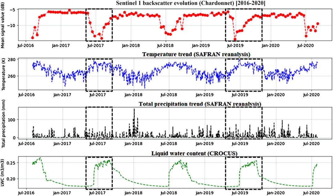
FIGURE 8. Joint analysis of the temporal backscattering profile for the IA on the north face of Chardonnet with meteorological parameters (air temperature, precipitation, and liquid water content).
Figure 9 shows the annual variation of the spatial CV values for three different land classes i.e., grass field, IA and ablation zone of a glacier. We notice that the CV values remain stable and consistent around a value of 1 (mean value 1.037) for the homogeneous surfaces (in this case, the grass field in Chamonix valley). The spatial CV values also fluctuate within the Rayleigh interval, indicating that homogeneity of the surface is maintained throughout the year. The highest CV values for the glacier ablation area (mean value = 2.089) represent a dynamic and spatially heterogeneous surface. For the IAs, the CV values fluctuate between those of spatially homogeneous and heterogeneous areas. The variation of the spatial CV values (mean CV = 1.25) indicates a quasi-stable surface (surfaces that might be homogenous at some intervals during the year). To better understand IAs characteristics, an analysis of the annual evolution of the spatial CV values was performed for 8 IAs located at a mean elevation of 3,468 m a.s.l. and visible in the PAZ images. In Figure 10, we notice that the CV values for none of the 8 IAs fall within the Rayleigh interval, which defines the zone of homogeneity as described in section 4.3. This implies that even though the IA surfaces (especially in winter) show values close to the Rayleigh interval during some months, they are never truly homogeneous. The mean spatial CV values show that the average CV values for 8 IAs are the highest in summer (1.55), while they are the lowest in winter (1.25). This is consistent with the observation in Figure 10:a gradual but noticeable increase in the CV values in summer and a decrease and more stable value in winter. The annual mean CV values in spring and fall are almost similar, 1.35 and 1.37, respectively. The mean value for the spatial CV for all IAs is 1.37. The increase in CV values in summer suggests increased heterogeneity of the surface of IAs, caused by the physical changes resulting from the changing meteorology. In section 5.2, we showed the effects of the increasing temperature on the backscattering response of IAs. By comparing the annual evolution of the backscattering responses of different IAs with the evolution of the CV, we would notice an inverse relationship. As backscattering signals drop in summer, the corresponding CV values increase. This is partly due to the surface melting of IAs and the possible exposure of strong scatterers like rocks on the IAs surface.
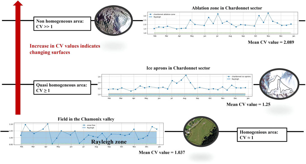
FIGURE 9. Three cases in temporal profiles with an increased coefficient of variation. The fully developed speckle class (field area), a signal indicating some radiometric changes (IAs), and a signal with extreme variations of CV values indicate rapidly changing heterogenous surfaces (ablation zone of active glaciers).
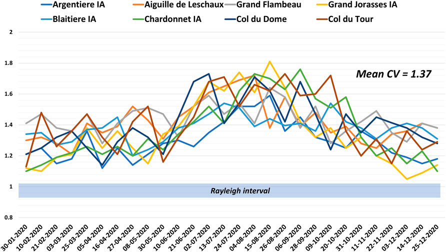
FIGURE 10. Annual evolution of the spatial coefficient of variation for 8 IAs using PAZ images.
The process of temporal interpolation and its necessity were described briefly in section 4.3. To confirm the success of the interpolation steps, we compared the signal variation from the original signal and the resampled signal for the IA on the NW face of Grand Flambeau (Figure 11). As can be seen from the results, both signals (original and resampled) show good conformity for most parts in backscatter values throughout the study period. The highest difference in backscatter values as observed was 0.02 in linear units. It can be assumed that such a difference will not significantly affect the final comparison results. Similar results were also observed for other areas tested. Hence, it is safe to suggest that the resampled Sentinel-1 images can be used for a fair comparison with the PAZ images without inducing a significant bias in the comparison results because of the interpolation.
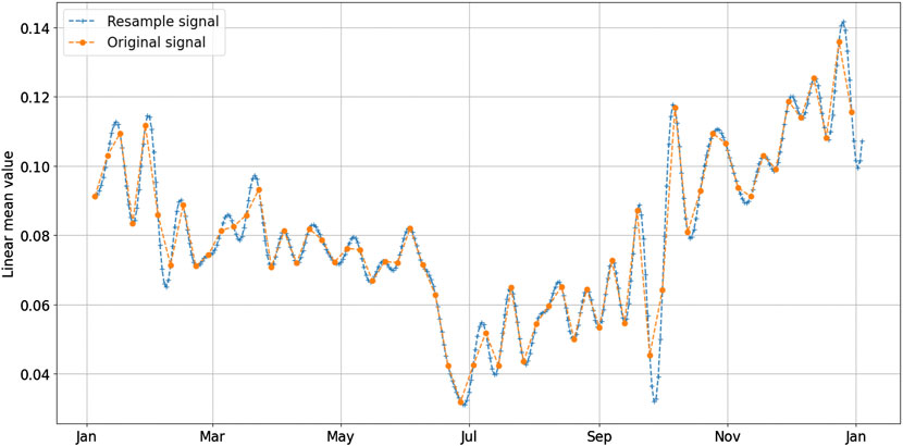
FIGURE 11. Comparison of the original Sentinel-1 signal with the resampled signal after temporal interpolation (we show an example for the IA on the NW face of Grand Flambeau).
Section 5.2 showed the evolution of backscattering signals in 2020 in X-bands and from 2016 to 2020 in C-band for different IAs. In this section, we try to quantitatively compare the evolution of the backscattering signals from Sentinel-1 and PAZ datasets in 2020 after resampling C-band time series at the X-band dates. According to the analysis, it is observed that for all IAs except for the IA on the N face of Col du Tour, the backscattering response in the case of the X-band is generally higher than that in the case of the C-band (Figure 12; Table 2). The average backscattering coefficient value for the 8 IAs is −9.22 dB with the X-band and −10.66 dB with the C-band. So the signal strength from the X-band is ∼1.4 dB higher than the same received from the C-band. Another observation is that the difference in the backscattering strength between the two bands is higher in winter than in summer. The best example of this is the IA trend on the N face of Argentiere, where the minimum value for the backscatter coefficient was observed in both the X-band (−17.50 dB) and C-band (−18.81 dB). The highest value is observed for the IA on the E face of Aiguille de Leschaux (−3.82 dB and—4.02 dB in the X- and C-band, respectively).
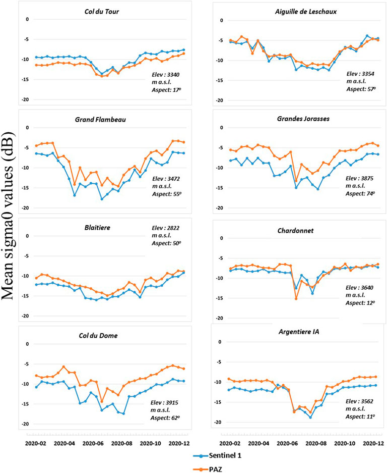
FIGURE 12. Comparison of the temporal backscattering profiles for 8 IAs in X-band PAZ and C-band interpolated Sentinel-1 images.

TABLE 2. Statistical analysis of X- and C-bands RaDAR backscattering for 8 different IAs.
The Pearson r value for the two annual trends shows a high correlation for all IAs. On the one hand, this indicates that the backscattering trend from both datasets is in good agreement. On the other, this also confirms the behaviour of the IAs with seasonal changes.
For the IAs, since the snow thickness is not substantial (generally less than the penetration depth of both X- and C-bands in dry snow), surface and shallow surface scattering phenomena seem to dominate. As the penetration depth of the C-band is higher than that of the X-band, surface and shallow surface volume scattering are almost undetectable for a few meters of dry snow surface compared to ground backscatter (Hall et al., 2005; Leinss et al., 2015). On the other hand, X-band has the highest sensitivity to surface changes; hence, changes on the surface of IAs cause an increase in backscattering signals more easily than with larger wavelengths. Moreover, below the thin layer of snow that accumulates in winter is a thick layer of ice that absorbs most of the penetrated RaDAR energy. This is another reason for the lower signal strength observed in the case of the C-band compared to the X-band.
This study was dedicated to understanding the physical backscatter properties of the IAs using X- and C-band RaDAR datasets. As a first result, we analyzed the seasonal variations of backscattering signals utilizing temporal profiles along with the Brenva glacier system. We noticed that the seasonal variations of the IAs were similar to that of the bare ice zone marked at the front of the glacier profile. Previous research has shown that the thickness of the IAs is not very significant and beneath the thin layer of snow which can accumulate on the surface of the IAs, is a highly metamorphosed layer of ice. Since the composition of the IAs is similar to the bare ice zone (except for the presence of crevasses and debris), we can expect a similar physical behaviour between the two glacier zones.
Further, a comparison of temporal backscatter trends for the 19 visible IAs in the PAZ images for 2020 shows a considerable drop in signal strength in summer. The same trend is also observed for a long term profile built with Sentinel-1 images since 2016. The backscatter trends corroborate with the meteorological changes observed during the same period. The sharp drop in backscatter relates directly to the melting of the snowpack, which leads to an increase in the liquid water content. A further comparison with the spatial coefficient of variation also shows that the CV values increase in the summer months and are most stable during the winters. The annual variation of the CV away from the Rayleigh interval strongly indicates the increase in heterogeneity, indicating significant surface changes. The results give the first indication from RaDAR images of the summer melting and surface change of IAs, which corroborates the previous findings of Kaushik et al. (2021a) and Guillet and Ravanel (2020) from optical images.
Further, we compared the backscatter response of 8 IAs zones in the X- and C-band. We observed that the average annual signal response from the IA was 1.4 dB higher than that from the accumulation zones with the X-band. We can conclude that IAs are more sensitive to the shorter wavelengths of the X-band than to the C-band. As the X-band is more sensitive to the surface and sub-surface variations, the physical processes of surface scattering dominate the physical response of IAs to RaDAR waves. This plausible explanation improves our understanding of the physical processes dominating the surface changes of IAs. This study is a first attempt focused solely on RaDAR images to improve our understanding of IAs, which are small but significant ice bodies overlooked by the scientific community. As a further continuation of this research, our enhanced understanding of the behaviour of the IAs should help researchers differentiate them from other parts of the glacial system. This research can also form the basis for the automatic classification of IAs in RaDAR images.
The raw data supporting the conclusions of this article will be made available by the authors, without undue reservation.
SK: Research development and Paper writing. BC: Data analysis and processing. ET, FK, YY, LR, and FM: Results interpretation and Paper proofreading.
The authors declare that the research was conducted in the absence of any commercial or financial relationships that could be construed as a potential conflict of interest.
All claims expressed in this article are solely those of the authors and do not necessarily represent those of their affiliated organizations, or those of the publisher, the editors and the reviewers. Any product that may be evaluated in this article, or claim that may be made by its manufacturer, is not guaranteed or endorsed by the publisher.
The authors thank the Spanish Instituto Nacional de Tecnica Aerospacial (INTA) for the PAZ images (Project AO-001–051).
Arigony-Neto, J., Rau, F., Saurer, H., Jaña, R., Simões, J. C., and Vogt, S. (2007). A Time Series of SAR Data for Monitoring Changes in Boundaries of Glacier Zones on the Antarctic Peninsula. Ann. Glaciol. 46, 55–60. doi:10.3189/172756407782871387
Ashcraft, I. S., and Long, D. G. (2006). Comparison of Methods for Melt Detection over Greenland Using Active and Passive Microwave Measurements. Int. J. Remote Sens. 27 (12), 2469–2488. doi:10.1080/01431160500534465
Awasthi, S., Kumar, S., Thakur, P. K., and Mani, S. (2017). “Pol-InSAR Based Snow Depth Retrieval Using Spaceborne TerraSAR-X Data,” in 2017 8th International Conference on Computing, Communication and Networking Technologies (ICCCNT) (Delhi: IEEE), 1–7. doi:10.1109/ICCCNT.2017.8204066
Bamber, J. L., and Rivera, A. (2007). A Review of Remote Sensing Methods for Glacier Mass Balance Determination. Glob. Planet. Change 59 (1–4), 138–148. doi:10.1016/j.gloplacha.2006.11.031
Berthier, E., Cabot, V., Vincent, C., and Six, D. (2016). Decadal Region-wide and Glacier-wide Mass Balances Derived from Multi-Temporal ASTER Satellite Digital Elevation Models. Validation over the Mont-Blanc Area. Front. Earth Sci. 4 (June), 63. doi:10.3389/feart.2016.00063
Berthier, E., Vincent, C., Magnússon, E., Gunnlaugsson, Á. Þ., Pitte, P., Le Meur, E., et al. (2014). Glacier Topography and Elevation Changes Derived from Pléiades Sub-meter Stereo Images. Cryosphere 8 (6), 2275–2291. doi:10.5194/tc-8-2275-2014
Brown, I. A., Kirkbride, M. P., and Vaughan, R. A. (1999). Find the Firn Line! the Suitability of ERS-1 and ERS-2 SAR Data for the Analysis of Glacier Facies on Icelandic Icecaps. Int. J. Remote Sens. 20 (15–16), 3217–3230. doi:10.1080/014311699211714
Bruder, J. A. (2013). IEEE Radar Standards and the Radar Systems Panel. IEEE Aerosp. Electron. Syst. Mag. 28 (7), 19–22. doi:10.1109/MAES.2013.6559377
Brun, E., Martin, Ε., Simon, V., Gendre, C., and Coleou, C. (1989). An Energy and Mass Model of Snow Cover Suitable for Operational Avalanche Forecasting. J. Glaciol. 35 (121), 333–342. doi:10.3189/S0022143000009254
Bühler, Y., Kumar, S., Veitinger, J., Christen, M., Stoffel, A., and Snehmani, (2013). Automated Identification of Potential Snow Avalanche Release Areas Based on Digital Elevation Models. Nat. Hazards Earth Syst. Sci. 13 (5), 1321–1335. doi:10.5194/nhess-13-1321-2013
Casey, J. A., Howell, S. E. L., Tivy, A., and Haas, C. (2016). Separability of Sea Ice Types from Wide Swath C- and L-Band Synthetic Aperture Radar Imagery Acquired during the Melt Season. Remote Sens. Environ. 174 (March), 314–328. doi:10.1016/j.rse.2015.12.021
Chan, A. K., and Peng, C. (2003). “Wavelets for Sensing Technologies,” in Artech House Remote Sensing Library (Boston: Artech House).
Chen, X., Sun, Q., and Hu, J. (2018). Generation of Complete SAR Geometric Distortion Maps Based on DEM and Neighbor Gradient Algorithm. Appl. Sci. 8 (11), 2206. doi:10.3390/app8112206
Cigna, F., Bateson, L. B., Jordan, C. J., and Dashwood, C. (2014). Simulating SAR Geometric Distortions and Predicting Persistent Scatterer Densities for ERS-1/2 and ENVISAT C-Band SAR and InSAR Applications: Nationwide Feasibility Assessment to Monitor the Landmass of Great Britain with SAR Imagery. Remote Sens. Environ. 152 (September), 441–466. doi:10.1016/j.rse.2014.06.025
Cooper, A. P. R. (2007). REMOTE SENSING of SNOW and ICE. W. Gareth Rees. 2005. Boca Raton, FL: CRC Press. Xx + 285 P, Illustrated, Hard Cover. ISBN 0-415-29831-8. £56.99; US$99.50. Polar Rec. 43 (1), 81–82. doi:10.1017/S0032247406255992
Dehecq, A., Millan, R., Berthier, E., Gourmelen, N., Trouve, E., and Vionnet, V. (2016). Elevation Changes Inferred from TanDEM-X Data over the Mont-Blanc Area: Impact of the X-Band Interferometric Bias. IEEE J. Sel. Top. Appl. Earth Obs. Remote Sens. 9 (8), 3870–3882. doi:10.1109/JSTARS.2016.2581482
Dietz, A. J., Kuenzer, C., Gessner, U., and Dech, S. (2012). Remote Sensing of Snow - a Review of Available Methods. Int. J. Remote Sens. 33 (13), 4094–4134. doi:10.1080/01431161.2011.640964
Durand, Y., Brun, E., Mérindol, L., Guyomarc'h, G., Lesaffre, B., and Martin, E. (1983). A Meteorological Estimation of Relevant Parameters for Snow Models. Ann. Glaciol. 18, 65–71.
Durand, Y., Laternser, M., Giraud, G., Etchevers, P., Lesaffre, B., and Mérindol, L. (2009). Reanalysis of 44 Yr of Climate in the French Alps (1958-2002): Methodology, Model Validation, Climatology, and Trends for Air Temperature and Precipitation. J. Appl. Meteor. Climatol. 48, 429–449. doi:10.1175/2008JAMC1808.1
Farinotti, D., Huss, M., Fürst, J. J., Landmann, J., Machguth, H., Maussion, F., et al. (2019). A Consensus Estimate for the Ice Thickness Distribution of All Glaciers on Earth. Nat. Geosci. 12 (3), 168–173. doi:10.1038/s41561-019-0300-3
Floricioiu, D., and Rott, H. (2001). Seasonal and Short-Term Variability of Multifrequency, Polarimetric Radar Backscatter of Alpine Terrain from SIR-C/X-SAR and AIRSAR Data. IEEE Trans. Geosci. Remote Sens. 39 (12), 2634–2648. doi:10.1109/36.974998
Forster, R. R., Isacks, B. L., and Das, S. B. (1996). Shuttle Imaging Radar (SIR-C/X-SAR) Reveals Near-Surface Properties of the South Patagonian Icefield. J. Geophys. Res. 101 (E10), 23169–23180. doi:10.1029/96JE01950
Fu, W., Li, X., Wang, M., and Liang, L. (2020). Delineation of Radar Glacier Zones in the Antarctic Peninsula Using Polarimetric SAR. Water 12 (9), 2620. doi:10.3390/w12092620
Gao, J., and Liu, Y. (2001). Applications of Remote Sensing, GIS and GPS in Glaciology: A Review. Prog. Phys. Geogr. Earth Environ. 25 (4), 520–540. doi:10.1177/030913330102500404
Gardent, M., Rabatel, A., Dedieu, J. P., and Deline, P. (2014). Multitemporal Glacier Inventory of the French Alps from the Late 1960s to the Late 2000s. Glob. Planet. Change 120 (September), 24–37. doi:10.1016/j.gloplacha.2014.05.004
Gelautz, M., Frick, H., Raggam, J., Burgstaller, J., and Leberl, F. (1998). SAR Image Simulation and Analysis of Alpine Terrain. ISPRS J. Photogrammetry Remote Sens. 53 (1), 17–38. doi:10.1016/S0924-2716(97)00028-2
Guillet, G., Preunkert, S., Ravanel, L., Montagnat, M., and Friedrich, R. (2021). Investigation of a cold-based ice apron on a high-mountain permafrost rock wall using ice texture analysis and micro-14C dating: a case study of the Triangle du Tacul ice apron (Mont Blanc massif, France). J. Glaciol. 67, 1205–1212. doi:10.1017/jog.2021.65
Guillet, G., and Ravanel, L. (2020). Variations in Surface Area of Six Ice Aprons in the Mont-Blanc Massif since the Little Ice Age. J. Glaciol. 66 (259), 777–789. doi:10.1017/jog.2020.46
Helfricht, K., Lehning, M., Sailer, R., and Kuhn, M. (2015). Local Extremes in the Lidar‐derived Snow Cover of Alpine Glaciers. Geogr. Ann. Ser. A, Phys. Geogr. 97 (4), 721–736. doi:10.1111/geoa.12111
Jezek, K. C., Drinkwater, M. R., Crawford, J. P., Bindschadler, R., and Kwok, R. (1993). Analysis of Synthetic Aperture Radar Data Collected over the Southwestern Greenland Ice Sheet. J. Glaciol. 39 (131), 119–132. doi:10.3189/S002214300001577X
Jezek, K. C. (1999). Glaciological Properties of the Antarctic Ice Sheet from RADARSAT-1 Synthetic Aperture Radar Imagery. Ann. Glaciol. 29, 286–290. doi:10.3189/172756499781820969
Johansson, A. M., Brekke, C., Spreen, G., and King, J. A. (2018). X-, C-, and L-Band SAR Signatures of Newly Formed Sea Ice in Arctic Leads during Winter and Spring. Remote Sens. Environ. 204 (January), 162–180. doi:10.1016/j.rse.2017.10.032
Joughin, I., Smith, B. E., and Abdalati, W. (2010). Glaciological Advances Made with Interferometric Synthetic Aperture Radar. J. Glaciol. 56 (200), 1026–1042. doi:10.3189/002214311796406158
Kääb, A., Bolch, T., Casey, K., Heid, T., Kargel, J. S., Leonard, G. J., et al. (2014). “Glacier Mapping and Monitoring Using Multispectral Data,” in Global Land Ice Measurements from Space. Editors J. S. Kargel, G. J. Leonard, M. P. Bishop, A. Kääb, and B. H. Raup (Berlin, Heidelberg: Springer Berlin Heidelberg), 75–112. doi:10.1007/978-3-540-79818-7_4
Kaab, A. (2008). Glacier Volume Changes Using ASTER Satellite Stereo and ICESat GLAS Laser Altimetry. A Test Study on EdgeØya, Eastern Svalbard. IEEE Trans. Geosci. Remote Sens. 46 (10), 2823–2830. doi:10.1109/TGRS.2008.2000627
Kaushik, S., Ravanel, L., Magnin, F., Yan, Y., Trouve, E., and Cusicanqui, D. (2021a). Distribution and Evolution of Ice Aprons in a Changing Climate in the Mont Blanc Massif (Western European Alps). Int. Arch. Photogramm. Remote Sens. Spat. Inf. Sci. XLIII-B3-2021 (June), 469–475. doi:10.5194/isprs-archives-XLIII-B3-2021-469-2021)
Kaushik, S., Yan, Y., Ravanel, L., Magnin, F., and Trouve, E. (2021b). “Visibility Analysis of Glaciers on Steep Slopes in the European ALPS Using Terrasar-X/PAZ Data,” in 2021 IEEE International Geoscience and Remote Sensing Symposium IGARSS (Brussels, Belgium: IEEE), 5505–5508. doi:10.1109/IGARSS47720.2021.9554966
Khaleghian, S., Ullah, H., Kræmer, T., Hughes, N., Eltoft, T., and Marinoni, A. (2021). Sea Ice Classification of SAR Imagery Based on Convolution Neural Networks. Remote Sens. 13 (9), 1734. doi:10.3390/rs13091734
King, J., Kelly, R., Kasurak, A., Duguay, C., Gunn, G., Rutter, N., et al. (2015). Spatio-Temporal Influence of Tundra Snow Properties on Ku-Band (17.2 GHz) Backscatter. J. Glaciol. 61 (226), 267–279. doi:10.3189/2015JoG14J020
Koeniguer, E. C., and Nicolas, J. M. (2020). Change Detection Based on the Coefficient of Variation in SAR Time-Series of Urban Areas. Remote Sens. 12 (13), 2089. doi:10.3390/rs12132089
König, M., Winther, J.-G., and Isaksson, E. (2001). Measuring Snow and Glacier Ice Properties from Satellite. Rev. Geophys. 39 (1), 1–27. doi:10.1029/1999RG000076
Kraaijenbrink, P. D. A., Bierkens, M. F. P., Lutz, A. F., and Immerzeel, W. W. (2017). Impact of a Global Temperature Rise of 1.5 Degrees Celsius on Asia's Glaciers. Nature 549 (7671), 257–260. doi:10.1038/nature23878
Kropatsch, W. G., and Strobl, D. (1990). The Generation of SAR Layover and Shadow Maps from Digital Elevation Models. IEEE Trans. Geosci. Remote Sens. 28 (1), 98–107. doi:10.1109/36.45752
Kundu, S., and Chakraborty, M. (2015). Delineation of Glacial Zones of Gangotri and Other Glaciers of Central Himalaya Using RISAT-1 C-Band Dual-Pol SAR. Int. J. Remote Sens. 36 (6), 1529–1550. doi:10.1080/01431161.2015.1014972
L3Harris Geospatial (2022). L3Harris Geospatial ENVI® SARscape®. Available at: https://www.harrisgeospatial.com/Software-Technology/ENVI-SARscape.
Lê, T. T., Atto, A. M., Trouvé, E., Solikhin, A., and Pinel, V. (2015). Change Detection Matrix for Multitemporal Filtering and Change Analysis of SAR and PolSAR Image Time Series. ISPRS J. Photogrammetry Remote Sens. 107 (September), 64–76. doi:10.1016/j.isprsjprs.2015.02.008
Leberl, F. W. (1984). A Review of: "Microwave Remote Sensing-Active and Passive". By F. T. Ulaby. R. K. Moore and A. K. Fung. (Reading, Massachusetts: Addison-Wesley, 1981 and 1982.) Volume I: Microwave Remote Sensing Fundamentals and Radiometry. [Pp. 473.] Price U.S. $46.50. Volume II: Radar Remote Sensing and Surface Scattering and Emission Theory. [Pp. 628.] Price U.S. $49.50. Int. J. Remote Sens. 5 (2), 463. doi:10.1080/01431168408948820
Li, H., Wang, Z., He, G., and Man, W. (2017). Estimating Snow Depth and Snow Water Equivalence Using Repeat-Pass Interferometric SAR in the Northern Piedmont Region of the Tianshan Mountains. J. Sensors 2017, 1–17. doi:10.1155/2017/8739598
Liu, H., Wang, L., and Jezek, K. C. (2006). Automated Delineation of Dry and Melt Snow Zones in Antarctica Using Active and Passive Microwave Observations from Space. IEEE Trans. Geosci. Remote Sens. 44 (8), 2152–2163. doi:10.1109/TGRS.2006.872132
Loibl, D., and Lehmkuhl, F. (2013). High-Resolution Geomorphological Map of a Low Mountain Range Near Aachen, Germany. J. Maps 9 (2), 245–253. doi:10.1080/17445647.2013.771291
Lubin, D., and Massom, R. (2005). “Polar Remote Sensing,” in Springer-praxis Books in Geophysical Sciences. 1st ed. (Berlin New York: Springer).
Lucas, G. R. (1995). Remote Sensing and Image Interpretation, 3rd Edn, by T. M. Lillesand and R. W. Kiefer, 1994. Wiley, Chichester. No. Of Pages: 750. Price: £19.95 (Paperback); £67.00 (Cloth). ISBN 0471 305 758. Geol. J. 30 (2), 204. doi:10.1002/gj.3350300217
Luckman, A., Quincey, D., and Bevan, S. (2007). The Potential of Satellite Radar Interferometry and Feature Tracking for Monitoring Flow Rates of Himalayan Glaciers. Remote Sens. Environ. 111 (2–3), 172–181. doi:10.1016/j.rse.2007.05.019
Magnin, F., Brenning, A., Bodin, X., Deline, P., and Ravanel, L. (2015). Modélisation statistique de la distribution du permafrost de paroi : application au massif du Mont Blanc. geomorphologie 21 (2), 145–162. doi:10.4000/geomorphologie.10965
Magnin, F., Etzelmüller, B., Westermann, S., Isaksen, K., Hilger, P., and Hermanns, R. L. (2019). Permafrost Distribution in Steep Rock Slopes in Norway: Measurements, Statistical Modelling and Implications for Geomorphological Processes. Earth Surf. Dynam. 7 (4), 1019–1040. doi:10.5194/esurf-7-1019-2019
Magnin, F., Westermann, S., Pogliotti, P., Ravanel, L., Deline, P., and Malet, E. (2017). Snow Control on Active Layer Thickness in Steep Alpine Rock Walls (Aiguille Du Midi, 3842ma.s.l., Mont Blanc Massif). CATENA 149 (February), 648–662. doi:10.1016/j.catena.2016.06.006
Marsh, O. J., Price, D., Courville, Z. R., and Floricioiu, D. (2021). Crevasse and Rift Detection in Antarctica from TerraSAR-X Satellite Imagery. Cold Regions Sci. Technol. 187 (July), 103284. doi:10.1016/j.coldregions.2021.103284
Masson, V., Le Moigne, P., Martin, E., Faroux, S., Alias, A., Alkama, R., et al. (2013). The SURFEXv7.2 Land and Ocean Surface Platform for Coupled or Offline Simulation of Earth Surface Variables and Fluxes. Geosci. Model. Dev. 6, 929–960. doi:10.5194/gmd-6-929-2013
Mätzler, C. (1987). Applications of the Interaction of Microwaves with the Natural Snow Cover. Remote Sens. Rev. 2 (2), 259–387. doi:10.1080/02757258709532086
Meier, W. J. H., Grießinger, J., Hochreuther, P., and Braun, M. H. (2018). An Updated Multi-Temporal Glacier Inventory for the Patagonian Andes with Changes between the Little Ice Age and 2016. Front. Earth Sci. 6 (May), 62. doi:10.3389/feart.2018.00062
Moen, M. A. N., Anfinsen, S. N., Doulgeris, A. P., Renner, A. H. H., and Gerland, S. (2015). Assessing Polarimetric SAR Sea-Ice Classifications Using Consecutive Day Images. Ann. Glaciol. 56 (69), 285–294. doi:10.3189/2015AoG69A802
Neckel, N., Kropáček, J., Bolch, T., and Hochschild, V. (2014). Glacier Mass Changes on the Tibetan Plateau 2003-2009 Derived from ICESat Laser Altimetry Measurements. Environ. Res. Lett. 9 (1), 014009. doi:10.1088/1748-9326/9/1/014009
Nefeslioglu, H. A., Sezer, E. A., Gokceoglu, C., and Ayas, Z. (2013). A Modified Analytical Hierarchy Process (M-AHP) Approach for Decision Support Systems in Natural Hazard Assessments. Comput. Geosciences 59 (September), 1–8. doi:10.1016/j.cageo.2013.05.010
Notti, D., Davalillo, J. C., Herrera, G., and Mora, O. (2010). Assessment of the Performance of X-Band Satellite Radar Data for Landslide Mapping and Monitoring: Upper Tena Valley Case Study. Nat. Hazards Earth Syst. Sci. 10 (9), 1865–1875. doi:10.5194/nhess-10-1865-2010
Partington, K. C. (1998). Discrimination of Glacier Facies Using Multi-Temporal SAR Data. J. Glaciol. 44 (146), 42–53. doi:10.3189/S0022143000002331
Patil, A., Mohanty, S., and Singh, G. (2020). Snow Depth and Snow Water Equivalent Retrieval Using X-Band PolInSAR Data. Remote Sens. Lett. 11 (9), 817–826. doi:10.1080/2150704X.2020.1779373
Phan, X. V., Ferro-Famil, L., Gay, M., Durand, Y., Dumont, M., Morin, S., et al. (2014). 1D-Var Multilayer Assimilation of X-Band SAR Data into a Detailed Snowpack Model. Cryosphere 8 (5), 1975–1987. doi:10.5194/tc-8-1975-2014
Quincey, D. J., Copland, L., Mayer, C., Bishop, M., Luckman, A., and Belò, M. (2009). Ice Velocity and Climate Variations for Baltoro Glacier, Pakistan. J. Glaciol. 55 (194), 1061–1071. doi:10.3189/002214309790794913
Rabatel, A., Letréguilly, A., Dedieu, J.-P., and Eckert, N. (2013). Changes in Glacier Equilibrium-Line Altitude in the Western Alps from 1984 to 2010: Evaluation by Remote Sensing and Modeling of the Morpho-Topographic and Climate Controls. Cryosphere 7 (5), 1455–1471. doi:10.5194/tc-7-1455-2013
Rabus, B. T., and Fatland, D. R. (2000). Comparison of SAR-Interferometric and Surveyed Velocities on a Mountain Glacier: Black Rapids Glacier, Alaska, U.S.A. J. Glaciol. 46 (152), 119–128. doi:10.3189/172756500781833214
Rafiq, M., and Mishra, A. (2016). Investigating Changes in Himalayan Glacier in Warming Environment: A Case Study of Kolahoi Glacier. Environ. Earth Sci. 75 (23), 1469. doi:10.1007/s12665-016-6282-1
Ramage, J. M., Isacks, B. L., and Miller, M. M. (2000). Radar Glacier Zones in Southeast Alaska, U.S.A. Field and Satellite Observations. J. Glaciol. 46 (153), 287–296. doi:10.3189/172756500781832828
Rastner, P., Prinz, R., Notarnicola, C., Nicholson, L., Sailer, R., Schwaizer, G., et al. (2019). On the Automated Mapping of Snow Cover on Glaciers and Calculation of Snow Line Altitudes from Multi-Temporal Landsat Data. Remote Sens. 11 (12), 1410. doi:10.3390/rs11121410
Rau, F., and Braun, M. (2002). The Regional Distribution of the Dry-Snow Zone on the Antarctic Peninsula North of 70˚ S. Ann. Glaciol. 34, 95–100. doi:10.3189/172756402781817914
Rignot, E., Rivera, A., and Casassa, G. (2003). Contribution of the Patagonia Icefields of South America to Sea Level Rise. Science 302 (5644), 434–437. doi:10.1126/science.1087393
Robinson, D., Kunzi, K., Kukla, G., and Rott, H. (1984). Comparative Utility of Microwave and Shortwave Satellite Data for All-Weather Charting of Snow Cover. Nature 312 (5993), 434–435. doi:10.1038/312434a0
Sam, L., Bhardwaj, A., Kumar, R., Buchroithner, M. F., and Martín-Torres, F. J. (2018). Heterogeneity in Topographic Control on Velocities of Western Himalayan Glaciers. Sci. Rep. 8 (1), 12843. doi:10.1038/s41598-018-31310-y
Sokol, J., Pultz, T. J., and Walker, A. E. (2003). Passive and Active Airborne Microwave Remote Sensing of Snow Cover. Int. J. Remote Sens. 24 (24), 5327–2344. doi:10.1080/0143116031000115076
Steffen, K., and Heinrichs, J. (2001). C‐band SAR Backscatter Characteristics of Arctic Sea and Land Ice during Winter. Atmosphere-Ocean 39 (3), 289–299. doi:10.1080/07055900.2001.9649682
Stiles, W. H., and Ulaby, F. T. (1980). The Active and Passive Microwave Response to Snow Parameters: 1. Wetness. J. Geophys. Res. 85 (C2), 1037. doi:10.1029/JC085iC02p01037
Strozzi, T., Luckman, A., Murray, T., Wegmuller, U., and Werner, C. L. (2002). Glacier Motion Estimation Using SAR Offset-Tracking Procedures. IEEE Trans. Geosci. Remote Sens. 40 (11), 2384–2391. doi:10.1109/TGRS.2002.805079
Strozzi, T., Wiesmann, A., and Mätzler, C. (1997). Active Microwave Signatures of Snow Covers at 5.3 and 35 GHz. Radio Sci. 32 (2), 479–495. doi:10.1029/96RS03777
Tadono, T., Nagai, H., Ishida, H., Oda, F., Naito, S., Minakawa, K., et al. (2016). Generation of the 30 M-Mesh Global Digital Surface Model by Alos Prism. Int. Arch. Photogramm. Remote Sens. Spat. Inf. Sci. XLI-B4 (June), 157–162. doi:10.5194/isprs-archives-XLI-B4-157-201610.5194/isprsarchives-xli-b4-157-2016
Taylor, L. S., Quincey, D. J., Smith, M. W., Baumhoer, C. A., McMillan, M., and Mansell, D. T. (2021). Remote Sensing of the Mountain Cryosphere: Current Capabilities and Future Opportunities for Research. Prog. Phys. Geogr. Earth Environ. 45 (June), 931–964. doi:10.1177/03091333211023690
Thakur, P. K., Garg, P. K., Aggarwal, S. P., Garg, R. D., and Mani, S. (2013). Snow Cover Area Mapping Using Synthetic Aperture Radar in Manali Watershed of Beas River in the Northwest Himalayas. J. Indian Soc. Remote Sens. 41 (4), 933–945. doi:10.1007/s12524-012-0236-1
Trantow, T., and Herzfeld, U. C. (2016). Spatiotemporal Mapping of a Large Mountain Glacier from CryoSat-2 Altimeter Data: Surface Elevation and Elevation Change of Bering Glacier during Surge (2011-2014). Int. J. Remote Sens. 37 (13), 2962–2989. doi:10.1080/01431161.2016.1187318
Waechter, A., Copland, L., and Herdes, E. (2015). Modern Glacier Velocities across the Icefield Ranges, St Elias Mountains, and Variability at Selected Glaciers from 1959 to 2012. J. Glaciol. 61 (228), 624–634. doi:10.3189/2015JoG14J147
Wiley, C. (1985). Synthetic Aperture Radars. IEEE Trans. Aerosp. Electron. Syst. AES-21 (3), 440–443. doi:10.1109/TAES.1985.310578
Winsvold, S. H., Kääb, A., Nuth, C., Andreassen, L. M., van Pelt, W. J. J., and Schellenberger, T. (2018). Using SAR Satellite Data Time Series for Regional Glacier Mapping. Cryosphere 12 (3), 867–890. doi:10.5194/tc-12-867-2018
Keywords: ice aprons, X-and C-band SAR, temporal backscattering profile, climate change, Mont Blanc massif
Citation: Kaushik S, Cerino B, Trouve E, Karbou F, Yan Y, Ravanel L and Magnin F (2022) Analysis of the Temporal Evolution of Ice Aprons in the Mont-Blanc Massif Using X and C-Band SAR Images. Front. Remote Sens. 3:930021. doi: 10.3389/frsen.2022.930021
Received: 27 April 2022; Accepted: 01 June 2022;
Published: 30 June 2022.
Edited by:
Wietske Bijker, University of Twente, NetherlandsReviewed by:
Muhammad Adnan Siddique, Information Technology University, PakistanCopyright © 2022 Kaushik, Cerino, Trouve, Karbou, Yan, Ravanel and Magnin. This is an open-access article distributed under the terms of the Creative Commons Attribution License (CC BY). The use, distribution or reproduction in other forums is permitted, provided the original author(s) and the copyright owner(s) are credited and that the original publication in this journal is cited, in accordance with accepted academic practice. No use, distribution or reproduction is permitted which does not comply with these terms.
*Correspondence: Suvrat Kaushik, c3V2cmF0LmswMDdAZ21haWwuY29t
Disclaimer: All claims expressed in this article are solely those of the authors and do not necessarily represent those of their affiliated organizations, or those of the publisher, the editors and the reviewers. Any product that may be evaluated in this article or claim that may be made by its manufacturer is not guaranteed or endorsed by the publisher.
Research integrity at Frontiers
Learn more about the work of our research integrity team to safeguard the quality of each article we publish.