Correction of inter-mission inconsistencies in merged ocean colour satellite data

Consistency in a time series of ocean colour satellite data is essential when determining long-term trends and statistics in Essential Climate Variables. For such a long time series, it is necessary to merge ocean colour data sets from different sensors due to the finite life span of the satellites. Although bias corrections have been performed on merged data set products, significant inconsistencies between missions remain. These inconsistencies appear as sudden steps in the time series of these products when a satellite mission is launched into- or removed from orbit. This inter-mission inconsistency is not caused by poor correction of sensor sensitivities but by differences in the ability of a sensor to observe certain waters. This study, based on a data set compiled by the ‘Ocean Colour Climate Change Initiative’ project (OC-CCI), shows that coastal waters, high latitudes, and areas subject to changing cloud cover are most affected by coverage variability between missions. The “Temporal Gap Detection Method” is introduced, which temporally homogenises the observations per-pixel of the time series and consequently minimises the magnitude of the inter-mission inconsistencies. The method presented is suitable to be transferred to other merged satellite-derived data sets that exhibit inconsistencies due to changes in coverage over time. The results provide insights into the correct interpretation of any merged ocean colour time series.

1 Introduction

Ocean colour is an Essential Climate Variable (ECV), as it captures various aspects of the marine environment on regional to global scales (GCOS, 2016). Earth observation of ocean colour is a widely used global quantitative measure to estimate optical constituents from derived reflectance. It includes the pigment chlorophyll-a concentration (hereafter “Chl-a”), the diffuse attenuation coefficient of downwelling irradiance (K_d490), as well as light absorption, and scattering coefficients (Kirk, 2011). Chl-a is used as a proxy of marine phytoplankton biomass and is responsible for approximately half of the global photosynthetic uptake of carbon dioxide (Field et al., 1998) and over half of the global oxygen production (Harris, 1986; Moss, 2009). Moreover, phytoplankton form the basis of the marine food web (Falkowski and Raven, 2001).

As of 2022, satellite-borne sensors have continuously measured ocean colour globally for more than 25 years. Continuity and data set stability are essential in climate research (GCOS, 2011). Because otherwise it is impossible to interpret the data as a continuous, time-integrated measurement of global climate. Spatio-temporal merging of ocean colour data sets optimise the spatial coverage and protects the temporal continuity of the data (IOCCG, 2007). Analysing trends using ocean colour data is challenging because of the relatively short lifespan (∼10 years) of a single satellite and large inter-annual and decadal variability of, e.g. the productivity of the ocean (Henson et al., 2010; Mélin, 2016; Hammond et al., 2018; Dutkiewicz et al., 2019). Each ocean colour sensor unique characteristics, such as overpass time and frequency, swath width, radiometric quality and stability, as well as spatial and spectral resolution. Moreover, data processed specifically for each sensor contain their own intrinsic uncertainties (IOCCG, 2019). Consequently, the construction of a multi-sensor merged data set is complex, and requires a deliberate approach as the merging must not result in inter-mission biases or artificial trends (Djavidnia et al., 2010; Gregg and Casey, 2010; Brewin et al., 2014; Mélin, 2016; Mélin et al., 2017; Sathyendranath et al., 2017). Approximately 40 years of data are required to distinguish the effect of a global warming trend on an ocean colour product, e.g., chlorophyll, from the natural variability of this product (Henson et al., 2010). Therefore, merging is necessary to be able to identify trends and other long-term statistics in ocean colour and obtain improved insight into the dynamics of phytoplankton and other optically active constituents in global waters. Although the total period of the current merged ocean colour data is probably not long enough for definite conclusions regarding climate change effects, it is essential to broaden our understanding of the consequences of merging data sets from different satellite missions.

Several initiatives exist that produce merged ocean colour data. These include the European Space Agency’s (ESA) Ocean Colour Climate Change Initiative (OC-CCI) (Sathyendranath et al., 2019), the ESA’s GlobColour project (globcolour.info) and the National Aeronautics and Space Administration’s (NASA) Making Earth Science Data Records for Use in Research Environments (MEaSUREs) project (measures.oceancolor.ucsb.edu). The OC-CCI version 5 data set provides global time series of several ECV products, including remote sensing reflectance (R_rs), Chl-a and inherent optical properties derived with common algorithms on homogeneous spectral reflectance data (Jackson, 2020; Sathyendranath et al., 2021). It consists of merged records originating from five different satellite sensors; SeaWiFS, MODIS and VIIRS by NASA/NOAA (United States), and MERIS and OLCI by ESA/EUMETSAT (Europe) on an equal-area grid. The resulting time series, ranging from September 1997 to June 2020, is designed to be the most internally consistent and stable ocean-colour record so far (Sathyendranath et al., 2019). Explicitly, the full data set is band-shifted to a common set of six spectral bands (that of MERIS) and corrected for inter-mission biases in the spectral response. However, ensuring multi-mission consistency sufficient to allow analysis of long-term statistical data remains a major task since the OC-CCI data set, as well as other multi-mission ocean colour data sets (e.g. GlobColour), are persistently spatio-temporally inconsistent (Hammond et al., 2018; Garnesson et al., 2019). Inter-mission inconsistencies appear as significant steps in global time series (Jackson, 2020) and seem to coincide with changes in the availability of single sensors. Similar patterns are found in numerous studies that use different merged ocean colour data sets (Kahru et al., 2012, 2015; Navarro et al., 2017; Sankar et al., 2019; Kulk et al., 2020; Joseph et al., 2021) and are potentially misinterpreted as a part of natural variability. Some phenology studies that use merged ocean colour data also show patterns concurring with mission availability (Gittings et al., 2021; Staehr et al., 2022). To prevent misinterpretation, it is necessary to confirm that these patterns are indeed caused by inter-mission inconsistencies, as opposed to a factual signal.

This study focusses on the OC-CCI-v5 data set because of its specific objective to produce a consistent data set suitable for climate science purposes (Jackson, 2020). Thereby, this data set has smaller inter-mission biases and better match-ups with in situ data compared to the GlobColour data set (Hammond et al., 2018; Jackson et al., 2021). Despite sophisticated in situ validation and inter-mission bias correction of the OC-CCI data set, clear steps are visible in global time series coinciding with the satellite mission(s) in orbit at that time. Our research aims to demonstrate that the different ability of the sensors to observe specific geographical pixels causes these significant inconsistencies. We show where coverage differences are most prominent and we present a method to achieve temporal consistency in every geographical pixel. The introduced solution is the “Temporal Gap Detection Method”, which improves the overall temporal homogeneity of satellite-derived data sets by correcting the differences in observational gaps per-pixel. It is particularly effective in coastal waters, high latitudes, and areas subject to changing cloud cover, which are commonly most affected by coverage inconsistencies between satellite sensors (Djavidnia et al., 2010). Moreover, this method is almost entirely independent of a specific variable, e.g., Chl-a, and can be transferred to other merged satellite data sets.

2 Description of inter-mission inconsistencies

2.1 Ocean colour-climate change initiative data set

This study uses daily products of the global OC-CCI data set (version 5) in a sinusoidal projection, with a spatial resolution of 1/24° at the equator (∼4.6 km globally) (Sathyendranath et al., 2021). The sinusoidal version is used because it does not increase weight in regions of high latitude due to spatial distortion as opposed to the geographic projection. The monthly composites presented in this study, are always produced by using all available daily values. The development and production of the OC-CCI data set are described in detail in the product user guide by Jackson (2020). We summarise the essential features of this guide in the next paragraph for better understanding, further discussion, and application in this paper.

2.1.1 Production of the data set

Optical satellite sensors measure radiance at the top of the Earth’s atmosphere. Atmospheric correction is necessary due to the large influence of the atmosphere on the relatively low signal from the water surface. The output is the remote sensing reflectance (R_rs) at the sea surface, which is the ratio of upwelling water-leaving radiance to downwelling irradiance. The atmospheric correction method POLYMER v4.1 (Steinmetz et al., 2011, 2016) is applied to all sensor data, except to data from SeaWiFS, where NASA’s l2gen processor (SeaDAS 7.5; Franz et al., 2007) is applied. Thereafter, the full data set is binned to level-3 on a 4 km sinusoidal grid with the BEAM binner developed by Brockmann Consult (brockmann-consult. de/cms/web/beam/). Then the binned data is flagged using a combination of l2gen and IdePix v6.0/v7.0 (brockmann-consult.de/portfolio/idepix/). After flagging, the data is band-shifted (Mélin and Sclep, 2015) to match six MERIS spectral bands (412, 443, 490, 510, 560, and 665 nm). Temporally weighted climatological maps are used to remove inter-mission biases per-pixel between the band-shifted R_rs products. VIIRS and OLCI are adjusted to MODIS-corrected-to-MERIS R_rs, as there is no temporal overlap between these two sensors and MERIS. Ultimately, all data are merged to a multi-sensor, daily R_rs data set. From this R_rs data set, several additional products are computed. Inherent optical properties (IOPs), such as the absorption coefficients of phytoplankton, a_ph, that of detritus plus coloured dissolved organic matter, a_dg, and that of total water constituents, a_tot are determined using the Quasi-Analytical Algorithm (QAA; Lee et al., 2009). The diffuse light attenuation coefficient, K_d, is calculated using the method created by Lee et al. (2005). Chl-a is estimated with a blend of diverse band ratio algorithms (OCI, OCI2, OC2, and OCx), weighted by the relative levels in optical water type classes (Moore et al., 2009). These classes are derived specifically for the OC-CCI-v5 data set. A table of uncertainties for each water type is computed from matchups with the OC-CCI in situ database (Valente et al., 2019). The percentage of the membership to each optical water type defines the weighted uncertainty for each pixel.

2.1.2 Differences in sensor data

Every sensor has a unique combination of temporal, spatial and spectral characteristics, which are summarised in Table 1. A single pixel in the combined data set contains observations from single or multiple sensors. Because of different overpass times, the merged data set consists of a combined product with observations occurring between 10.00 and 13.30 local time. This may have consequences in areas that show strong diurnal variability (IOCCG, 2007; IOCCG, 2019).

TABLE 1

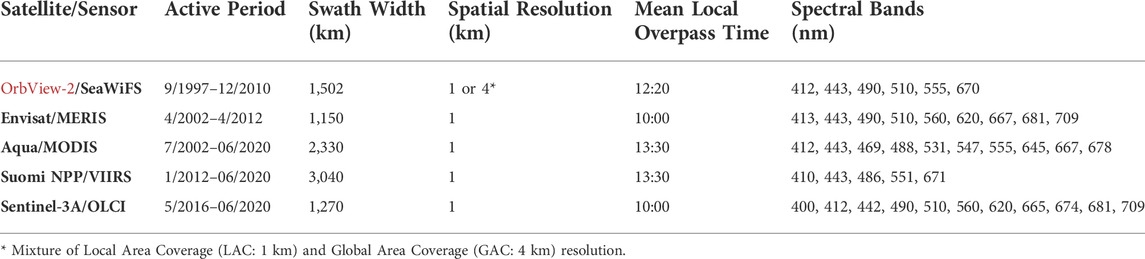
TABLE 1. Overview of satellite missions used in the OC-CCI data set. The spatial resolution is given for values prior to combining the data sets from the different missions (from Jackson, 2020).

SeaWiFS Global Area Coverage (GAC) may contribute ∼16 times fewer observations per 4-km-pixel compared to the other sensors in the data set, because SeaWiFS GAC has a spatial resolution of 4 km, whereas the other sensors and SeaWiFS Land Area Coverage (LAC) have a spatial resolution of 1 km before binning (Jackson, 2020). VIIRS has the largest swath width and therefore covers a larger area compared to the other sensors. Consequently, it provides a relatively large number of daily observations (Figure 1A).

FIGURE 1

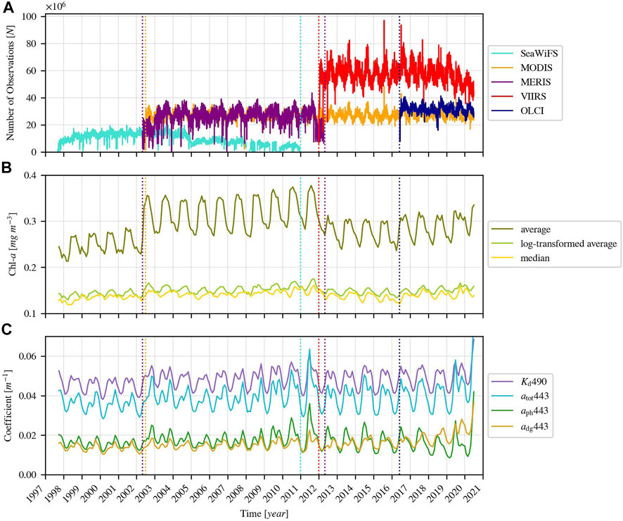
FIGURE 1. Time series of global OC-CCI data: (A) Sum of pixels daily observed by each sensor (see legend), globally (B) Monthly-averaged and median Chl-a: shown are the original monthly mean, median and “logarithmically transformed” mean (see text for details) (C) Monthly-averaged diffuse attenuation coefficient at 490 nm, K_d490, and total-, phytoplankton-, and detritus + gelbstoff absorption coefficients at 443 nm, a_tot, a_ph, a_dg, respectively (see legend). Vertical lines indicate times when the combination of active sensors has changed (see Table 1).

SeaWiFS is the only sensor that is atmospherically corrected with the l2gen algorithm (Franz et al., 2007) in the OC-CCI data set. Because the OC-CCI group decided to utilise the best individual atmospheric correction per sensor but are increasingly using the same atmospheric correction to provide consistency (Groom et al., 2022). The other sensors are atmospherically corrected using POLYMER based on pixel-by-pixel spectral optimisation. One feature of POLYMER is that it provides stable R_rs under moderate Sun glint. L2gen, on the other hand, is based on the estimation of the path radiance in near-infrared spectral bands using a linear model. It masks Sun glint affected pixels and hence significant parts of the swath (see Müller et al., 2015b). Brewin et al. (2014) found that using POLYMER or l2gen results in ∼90% significant correlation between the atmospherically corrected global Chl-a data sets. Areas that show a lower correlation between POLYMER and l2gen processed MERIS Chl-a data sets are located in minimal cloud-covered regions that generally have a weak seasonality in Chl-a, such as the Sargasso Sea and the North Pacific subtropical gyre. Djavidnia et al. (2010) reported similar patterns when comparing MERIS to either MODIS or SeaWiFS. Djavidnia et al. (2010) attribute the differences between Chl-a values, measured by the different sensors, to the sensitivity of the final product to the geometry of the seasonal cycle of solar illumination in the atmospheric correction. High solar zenith angles cause larger discrepancies between the R_rs product of SeaWiFS, MODIS and VIIRS (Barnes and Hu, 2015).

Pixel classification (or flagging) is used to determine whether a satellite observation is suitable for processing (Sathyendranath et al., 2019). All the OC-CCI sensor data were analysed using IdePix. Since the SeaWiFS L2 data are processed with SeaDAS, an extra flagging step has been applied to these data (Jackson, 2020). This additional flagging for invalidity includes areas experiencing glint, cloud shadows, brightness, and high solar and sensor zenith angles (Müller et al., 2015a).

2.2 The remaining inter-mission inconsistencies

Despite the many efforts made to remove inter-mission biases, some inconsistencies inevitably remain (Mélin et al., 2016; Jackson, 2020). Even though trends in the OC-CCI-v3 data set are consistent compared to single missions (Mélin et al., 2017), major discontinuities in the OC-CCI data set are present, corresponding to the introduction or discontinuation of a specific sensor (Hammond et al., 2018). The level of agreement between the Chl-a estimates by different sensor data sets varies temporally and geographically (Djavidnia et al., 2010; Brewin et al., 2014; Hammond et al., 2018). High latitude, coastal regions, areas with high cloud cover and those with high aerosol loads show, in general, the largest differences in Chl-a between the different sensors. Some areas show clear seasonal patterns of inter-mission inconsistencies (Gregg and Casey, 2007; Djavidnia et al., 2010). Additionally, different spatial sampling rates of the sensors may affect long-term trend detection (Brewin et al., 2014). These studies did not use the OC-CC-v5 data set, but we consider them relevant because the sensors included are similar and the construction method has not changed significantly between the different OC-CCI data set versions.

Few studies have produced time series of Chl-a on a global or regional scale using version 5 of the OC-CCI data set (Kulk et al., 2020; Joseph et al., 2021). The consistency of the version 5 data set shows some limitations, as steps were found in the Chl-a/primary production time series, coinciding with the time that MERIS commenced in April 2002 and discontinued in April 2012. Jackson (2020) reported inter-mission inconsistencies, appearing as such significant steps in the global monthly-averaged Chl-a time series. These were attributed to the increase in coverage of highly productive coastal regions by MERIS and the processing of MERIS data with POLYMER. Multiple ocean colour products, including the fundamental remote sensing reflectance, show these steps in the monthly-averaged time series (Figures 1B,C). Application of logarithmical transformation was suggested by several studies to reduce effects of high Chl-a values on statistics (Campbell, 1995; Brewin et al., 2014; Jackson, 2020). In these studies, logarithmical transformation refers to transforming the original Chl-a data set to its natural logarithm, which is then averaged and transformed back to a normal distribution. We will not use logarithmical transformation in this study because we are specifically interested in the inconsistencies in merged satellite data sets. Above that, by applying logarithmical transformation to the data set, these inconsistencies are still present (Figure 1B). We also focus on Chl-a from here on, because it is the variable with the best in situ validation (Valente et al., 2019) and it is the most widely used ocean colour product. Note that the gradual increase at the end of the time series in both Figures 1B,C is an artefact that arises during the production of the OC-CCI data set. This problem not yet solved and the consequences of this artefact are not yet established, but is beyond of the scope of this study.

3 Methods

The irregular spatio-temporal coverage of ocean colour sensors can result in bias when producing statistics (Gregg and Casey, 2007). A previously un-investigated cause of inconsistencies between data from different missions could be the different ability of the sensors to observe specific geographic positions (pixels) consistently in time. Therefore, we investigate non-random observation gaps over the seasons for all geographical pixels and present a new method to homogenise merged data sets temporally.

3.1 Temporal gap detection method

The Temporal Gap Detection Method (TGDM) is introduced to enable the construction of an annually equally represented daily time series for every geographical pixel. Each day within the data of a pixel is scanned for observation availability in a time window of ±n days of a respective day. If there are no observations for that day or in the temporal vicinity (the time window around), this day of the year is masked out in every year for the selected geographical pixel. The following steps illustrate the method in more detail for one random pixel (56° 56′ N, 4° 21′ E) located in the North Sea (see Figure 2):

1) The black markers in Figure 2A illustrate all observations in this geographical pixel. There are no observations in the middle of the winter at any point in time, because, the solar zenith angle at local noon is too large (∼80°) at its location of 56° 56′ N. Therefore, the signal-to-noise ratio of the radiance used to calculate the reflectance from the satellite sensor is too low (IOCCG, 2000). Furthermore, it is mostly cloudy here in winter.

2) A time window is moving over every day of the geographic pixel. Within this time window (and its selected day), the amount of observations are summed (Figure 2B). The length of the time window used in this example is 27 days, 13 before and 13 after the specific day. The time window length of 27 days is determined by optimisation, which is described in Section 3.2. A day is marked red if it did not receive any observations on the day itself, nor in its corresponding time window. These observational gaps are generally slightly longer during the first period (9/1997–4/2002), when only the SeaWiFS sensor was active.

3) The summed observations time series in Figure 2B is rearranged to a “day of the year” composition in Figure 2C where the lowest value over all years is taken. The red marked days did not receive any observations for that day of the year (plus its time window) in at least one of the years in the full time series. These days of the year are masked in every year of the full time series. As a result, the time series is no longer affected by missing observations in individual years. Another consequence is that certain time intervals of the year are no longer visible. The pixel in this example has been observed consistently in the local spring and summer months but not in the winter and not during minor gaps around days 90 and 200.

4) The blue markers below the original observations in Figure 2A represent the observations that are kept after temporal filtering using the TGDM. For this specific example of a single pixel, 81% of the total observations remain after applying the TGDM.

FIGURE 2

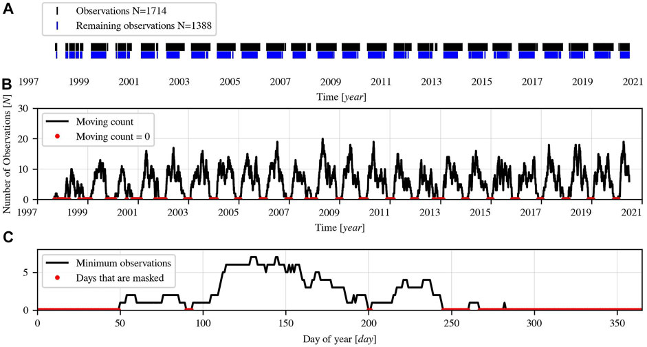
FIGURE 2. The Temporal Gap Detection Method (TGDM) applied as a showcase to one pixel located in the North Sea (using a time window length of 27 days): (A) Original observations for this pixel (in black) and those remaining after TGDM is applied (in blue). (B) Full time series of the summed number of observations for this pixel within the time window calculated per day. Time periods without observations are marked in red. (C) The minimum number of observations of the full time period shown in (B) as a function of the ‘Day of year’. Days of the year without observations (in red) are masked in every year for the full time series.

A hypothetically fully observed geographical pixel in the OC-CCI-v5 data set contains N = 8,336 daily data records. Consequently, the TGDM method could potentially mask ∼4.3% data records for every non-observed day of the year in a geographical pixel (length of data set: ∼23 years). However, this is not the amount that is typically lost, since pixels are not observed daily. The mean number of observations per pixel is substantially lower, namely, N = 978 globally. The pixel used in Figure 2 (N = 1714) contains ∼21% of observations compared to being fully observed. After applying the TGDM to this specific pixel, ∼17% of records are kept (N = 1,388) compared to a hypothetically fully observed pixel. The masked data masked are not bad data but potentially distort a time series due to inhomogeneity over time.

3.2 Finding the optimal time window length

The determination of the time window length presents an optimisation problem. Our objective is to determine the optimal reduction of the magnitude of the inter-mission inconsistencies in the time series caused by coverage differences and its coupled time window length. A too long time window length may not reduce the inconsistencies sufficiently, whereas a time window that is too short results in excessive removal of observations. The global, monthly Chl-a time series based on the median is used for optimisation because it is generally less variable and less susceptible to outliers compared to a time series based on the mean.

3.2.1 Magnitude of inter-mission inconsistencies

The magnitude of the steps in the time series of Chl-a caused by inter-mission coverage changes (hereafter Simc) is quantified by estimating the difference between the sub-periods and the corresponding times of the full period. The Simc can also be estimated by using another variable than Chl-a. An adapted version of standard deviation is used to calculate Simc:

1) The Chl-a time series is divided into four broad sub-periods. These sub-periods are defined as; the first period when only SeaWiFS is available in orbit (9/1997–4/2002), the second period when MERIS and MODIS join (5/2002–4/2012), the third period when VIIRS is launched and MERIS terminates (5/2012–5/2016) and the fourth period when OLCI joins the time series (6/2016–6/2020).

2) The trend lines of the monthly mean or median Chl-a time series of the full period and the four sub-periods are estimated by decomposition into a trend-, seasonal- and residual-component with Seasonal-Trend decomposition using Loess (STL) (Cleveland et al., 1990).

3) Linear least-squares regression analysis is performed to produce regression lines of the trend lines of the full period and the four sub-periods.

4) The differences between the means of the regression lines of the sub-periods ($C_{1i}$) and the means of corresponding parts ($C_{2i}$) of the regression line of the full period are calculated and squared.

5) The Simc is quantified by taking the square root from the mean of these four squared differences.

The associated equation is

$Simc =\sqrt{\frac{{{\displaystyle \sum }}_{i=1}^P{(C_{1i} - C_{2i})}^2}{P}},(1)$

where Simc is the magnitude of the steps in the time series of Chl-a caused by inter-mission coverage changes, $C_{1i}$ the average Chl-a of the regression lines of the sub-periods, $C_{2i}$ the corresponding sub-periods of the regression line of the full period, and $P$ is the number of sub-periods ($P$ =4, in this study).

3.2.2 Optimisation

The TGDM is applied to the global Chl-a data repeatedly, using a gradually increasing (+ 2 days) time window length between 15 (1+2 × 7) days and 365 (1+2 × 182) days. The Simc is calculated for each time window length. A threshold value is introduced, which is defined as the standard deviation of the residuals time series (estimated with LOESS). The Simc is deemed sufficiently low when it matches this threshold value. The corresponding time window length to this Simc and threshold value is used for the TGDM as the optimal time window length.

3.3 Validation methods

It is well known that specific geographical areas, such as coastal regions or regions at higher latitudes, consist of waters with varying phytoplankton concentrations. For a time series that analyses such areas, it is crucial that the observed part of the area is not changing with each active sensor. As an example, MERIS provided data from higher latitudes than other sensors. Consequently, during the period when MERIS is active, the observed area at higher latitudes increases compared to the period when MERIS is not available. The coverage of an area should be as homogeneous as possible over time to avoid inconsistencies. Inter-mission coverage differences should therefore be minimised after applying the TGDM. The OC-CCI data set includes products of the observation count for every sensor. These are used to derive the per-sensor contribution to a pixel. The average count of observations per month in a pixel for every sensor is calculated for the original- and the temporally homogenised data set. The dependency of the observation count (before and after TGDM) on the distance to coast, latitude, and latitude in December is determined. December was chosen to show the effect of adverse viewing geometries during mid-winter at Northern latitudes. This validation method is independent since the TGDM–except for optimisation–does not use information from the sensor observation variables (e.g., Chl-a).

A second validation method is carried out to confirm whether the TGDM performs similarly on densely- and scarcely covered areas. An example with data from the Mediterranean Sea is used because it is one of the most densely covered areas in the OC-CCI data set. A second data set of the Mediterranean Sea is prepared with an artificially diminished coverage density. The TGDM is then applied to the original- and the artificial Mediterranean Sea data set. If the Simc is reduced similarly in the time series of both data sets, the coverage density of the area has an insignificant influence on the functioning of the TGDM.

This artificial Mediterranean Sea data set is prepared by introducing data gaps along the date dimension in every geographical pixel. These data gaps were not randomly chosen. Instead, the irregularly and scarcely observed Bay of Bengal is used as a reference to create the observational gaps for every date per geographic pixel. The coordinate indices of the Bay of Bengal region are reconstructed artificially to match the coordinate indices of the Mediterranean Sea with a similar distance to the coast. The date dimension of each geographical pixel in the Mediterranean Sea is compared to the accompanying “Bay of Bengal pixel”. If a “Bay of Bengal pixel” does not contain data for a certain date, the observation of that day is removed in the related “Mediterranean Sea pixel”. This results in a heavily diminished coverage density in the artificial Mediterranean Sea data set because now it contains significant observational gaps.

3.4 Data set without SeaWiFS

The goal of the TGDM is to make the distribution of observations per geographic pixel more similar for all years and therefore periods (>1 year) with the fewest observations are limiting. Consequently, the resulting coverage after applying the TGDM is mainly determined by the first period (09/1997–04/2002) in the OC-CCI data set. It contains the poorest coverage during this time, since SeaWiFS is the sole active mission (Figure 1A). This directly affects the days of the year that are masked in every geographical pixel during the full period. Since it is impossible to acquire additional data during this time, because this data does not exist, the only way to increase coverage density for the full data set is to either accept a larger Simc or to exclude this first period. The length of the time series is shortened significantly when removing this first period. However, for some studies coverage density may be more important than the length of the time series. The TGDM is applied to the data set without the inclusion of the first period, to assess the increased coverage density.

4 Results

4.1 Time window length

4.1.1 Effects on the data set

Using not only a single day in question to homogenise the data set but also allowing observations in a time window around that day leads to fewer masked observations. The length of the time window influences the number of pixels and the associated Chl-a values that are masked. Figure 3 shows a strong sensitivity of the rigorousness of the mask to high Chl-a values: a small time window length (a strong cut) of 15 days leaves only ∼50% of pixels with low Chl-a and ∼10% of pixels with high Chl-a (>40 mg m⁻³). Using a relatively long time window length of 149 days, leaves ∼100% of the pixels with low Chl-a and ∼35% of pixels with Chl-a above 40 mg m⁻³.

FIGURE 3

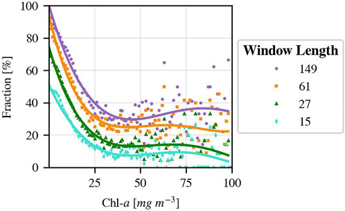
FIGURE 3. The fraction of data remaining compared to the full data set after applying the TGDM as a function of Chl-a and used time window length (in days). Lines represent the results of polynomial fits.

4.1.2 Optimal time window length

Figure 4 shows the trend line of the original global Chl-a, determined by STL decomposition of the monthly median time series. The calculated Simc of this trend line is 0.0039 mg m⁻³, which is almost twice the calculated threshold value of 0.0026 mg m⁻³. Figure 5 shows that after applying the TGDM, the Simc can be reduced to <0.0015 mg m⁻³ with a time window length of 15 days. By using this time window length, 61% of the records in the data set are masked. If a time window length of 365 days is used, 1% of the data records are masked and the corresponding Simc is 0.0035 mg m⁻³. The Simc increases rapidly from 15 until a time window length of approximately 50 days. After that, the Simc does not increase much further (Figure 5). The Simc surpasses the threshold value at a time window length of 27 days. Therefore, a time window length of 27 days is used in the following analysis. With a cut based on this time window length, 30% of all data are masked. The masked pixels contain a large proportion of high Chl-a values (see Figure 3).

FIGURE 4

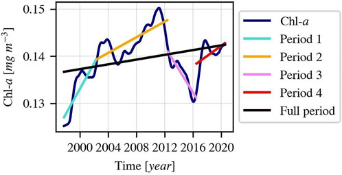
FIGURE 4. The trend component, derived with STL, of the global, monthly median Chl-a time series. Additionally shown are linear regression lines for the full period of OC-CCI data and the four sub-periods of varying mission combinations: 1: SeaWiFS only, 2: +MODIS/MERIS, 3: MERIS/+VIIRS, 4: +OLCI.

FIGURE 5

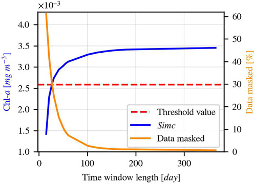
FIGURE 5. The magnitude of the inter-mission inconsistencies of the Chl-a (Simc) in the global time series as a function of time window length (blue) used in the TGDM (see text for details) and the coupled amount of data records masked after TGDM (orange). The dashed red line represents a threshold value defined by the standard deviation of the noise in the time series.

4.2 Validation of TGDM

4.2.1 Coverage area and timing

The top panels (A, B, and C) in Figure 6 show that differences in coverage between different ocean colour sensors are found in terms of latitude, seasonality and distance to the coast in the original data set. In the northern hemisphere, VIIRS does not observe pixels further north of 82.5° N, while MERIS observes the most northerly pixels, and reaches 86.5° N. In the winter months, SeaWiFS is the most limited sensor; in December, it reaches ∼48° N, whereas other satellite sensors extend to ∼54° N. These differences in latitudinal coverage arise from the individual restriction of acceptable Sun zenith angles in the data processing chain of each sensor. For comparison, all satellite missions reach a similar latitude - up to approximately 79.5° S - because of Antartica’s land and ice masses in the Southern Hemisphere (data not shown). OLCI has the highest monthly mean of observations per-pixel located nearest to the coast (4.9) and SeaWiFS the least (2.4). The bottom panels (D, E, and F) in Figure 6 show that the application of the TGDM to the original data set successfully reduces the differences in coverage between sensors. The maximum latitudes where pixels are observed have equalised in both the data set of the full time series and that of only December. The coverage differences related to the distance to the coast have become more equal (Figure 6D) as the range between the least mean observations per month nearest to the coast by SeaWiFS (3.1) and the most observations by VIIRS (4.5) has decreased. The corresponding mean Chl-a values of the different sensors at the pixels nearest to the coast have equalised from a range of 2.7–3.8 to 2.1–2.4 mg m⁻³ (see Table 2). MERIS has the highest average Chl-a near the coast (3.8 mg m⁻³) and SeaWiFS the lowest (2.7 mg m⁻³) in the original data set. The highest values of Chl-a were masked in all sensors after applying the TGDM, which is expected from the results shown above (Figure 3).

FIGURE 6

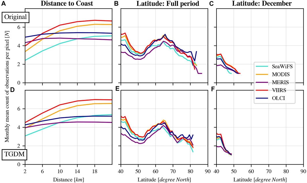
FIGURE 6. Global monthly-averaged number of observations per pixel for each satellite sensor (see legend) as a function of: the pixel centre’s distance to the coastline (binned on 4 km and the x-axis shows the bin centre) (A,D), the latitude for the full period (binned on 1° for the northern hemisphere) (B,E), and the latitude for only the northern winter month December (C,F). Shown are the results for the original data set (top: (A–C) and the data set after applying the TGDM (bottom: (D–F).

TABLE 2

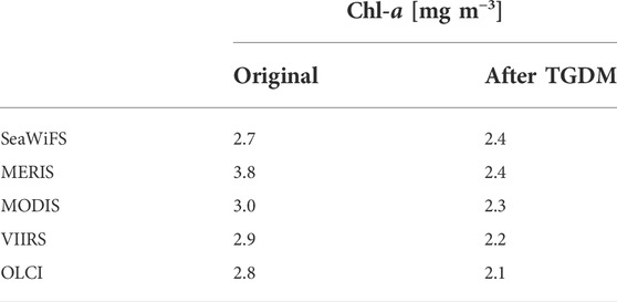
TABLE 2. The average Chl-a per sensor of the pixels nearest to the coast (centre of the pixel located between 0 and 4 km from the coastline) of the original data set and the temporally homogenised data set (i.e. after applying the TGDM).

4.2.2 Coverage density

The original monthly-averaged Chl-a time series of the Mediterranean Sea is shown in Figure 7A. The time series of the Mediterranean Sea data set, which had its coverage density artificially diminished, is shown in Figure 7B. The “artificial” data set consists of only 18.6% of the number of observations compared to the original data set. In both time series, the initial Simc’s are the same: ∼0.021 mg m⁻³ Figures 7C,D demonstrate that the inter-mission inconsistencies in the monthly-averaged Chl-a time series are minimised after the TGDM. The percentage of data kept of the original Mediterranean Sea data set after applying the TGDM is 97.7%. The number of observations in the artificial Mediterranean data set is reduced to 26.3%. This means that a significant number of observations in the artificial data set is masked to achieve temporal consistency. The Simc is now minimised to 0.005 mg m⁻³ for the original time series and to 0.006 mg m⁻³ for the artificial time series. Hence, the initial Simc’s and the Simc’s after applying the TGDM are similar for both the Mediterranean Sea and the artificial Mediterranean Sea. This shows that coverage density does not significantly affect the Simc and thus the behaviour of TGDM.

FIGURE 7

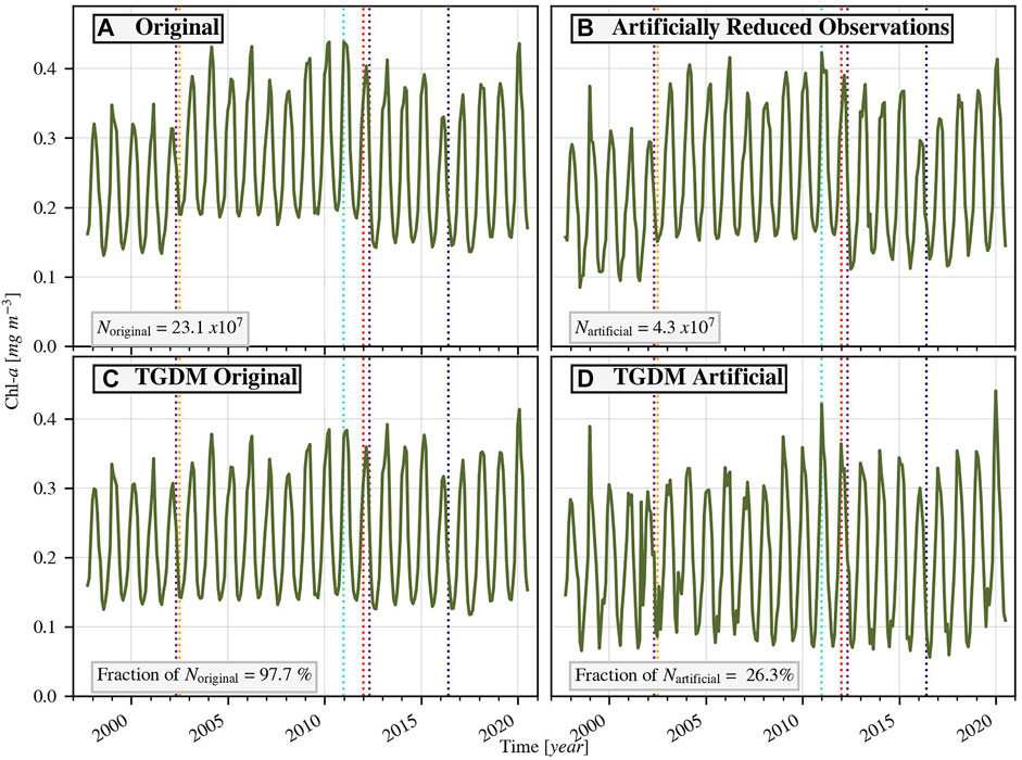
FIGURE 7. The performance of the TGDM on data sets with differing coverage densities: (A) The monthly-averaged Chl-a time series of the Mediterranean Sea and (B) the Mediterranean Sea data set with artificially reduced observations. The indicated numbers N_original and N_artificial represent the total count of observations. Panels (C) and (D) represent the monthly-averaged Chl-a time series after applying the TGDM to the original Mediterranean Sea and the artificial Mediterranean Sea, respectively. The fractions of the total observations that remain after TGDM are indicated as “Fraction of N”. Vertical lines indicate changes in sensor contributions (colouring specified in Figure 1).

4.3 Temporally homogenised data set

The original time series of monthly-averaged global Chl-a clearly shows the inter-mission inconsistencies (Figure 8A). After applying the TGDM, the Simc is reduced from 0.024 mg m⁻³ to 0.004 mg m⁻³ (see Table 3). The original and the temporally homogenised time series ofChl-a are shown in Figures 8B–D for the regions north of the tropics (>23° 26′ N), the tropics (23° 26′ N to 23° 26′ S) and south of the tropics (>23° 26’ S), respectively. These regions are chosen to separate the data set into areas with similar solar geometries. The Simc in the original Chl-a time series during the MERIS period is particularly pronounced north of the tropics and the tropics (Figures 8B,C, respectively). The smaller Simc south of the tropics (Figure 8D) is likely caused by the lower number of coastal shelve pixels in this region as well as the latitudinal observational reach of the satellites is distributed more equally here. The Simc is minimised in all regions after applying the TGDM. The TGDM improves the Simc more in tropics and north of the tropics compared to south of the tropics because Simc is more pronounced in these regions in the original data set. The average of Chl-a also decreased in the global data set and its subsets, especially during the period when MERIS is active. MERIS is able to observe more pixels near the coast, i.e., from regions with a generally higher productivity. Hence, the MERIS data contain more coastal pixels with high Chl-a values. As observations near the coast, consisting of higher Chl-a values, are masked when applying the TGDM, the variability in the data set is slightly reduced. The monthly median Chl-a time series is lower and less seasonally variable than the mean time series, because the values are (nearly) log-normally distributed (Campbell, 1995). This generally results in a lower Simc in the median time series compared to the Simc of the average time series (Table 3).

FIGURE 8

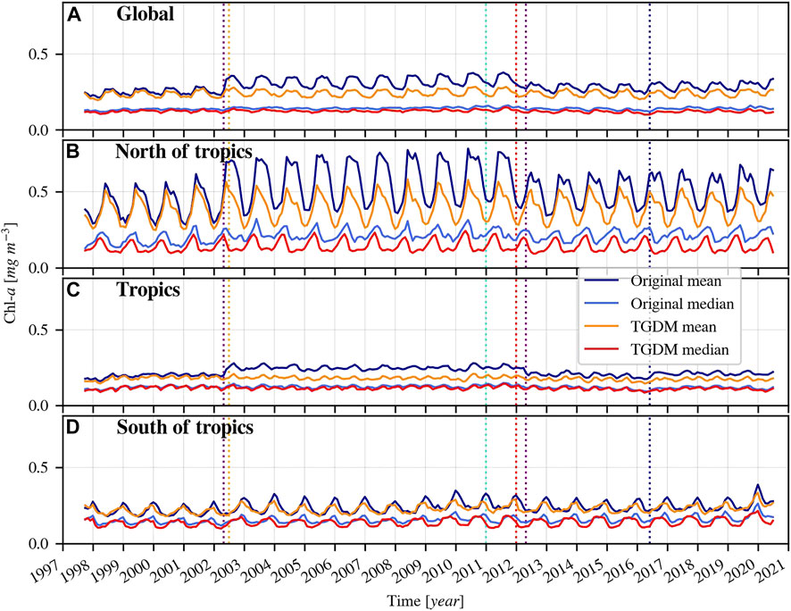
FIGURE 8. Time series of the monthly mean and median Chl-a before and after applying the TGDM: (A) global (B) north of the tropics (C) the tropics, and (D) south of the tropics. Vertical lines indicate changes in sensor contributions (colouring specified in Figure 1).

TABLE 3

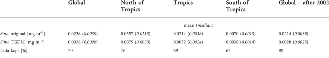
TABLE 3. TGDM effect on the magnitude of the inconsistencies (Simc) of the Chl-a time series (monthly mean and median) and data kept compared to the original data set for several subsets (geographical and temporal).

After applying the TGDM, 70% of the observations in the global data set remain (Table 3). Regional differences are large (Figure 9A) because of the different capabilities of the sensors to observe specific pixels. Somewhat counterintuitively, more observations are masked south of the tropics (67%) as opposed to north of the tropics (76%), while the Simc is considerably larger north of the tropics. This may be explained by the large number of pixels masked in the latitudes south of 40° S, which are often covered by clouds, but are quite constant in terms of variability within the ocean colour product. The Intertropical Convergence Zone (ITCZ) is clearly visible in Figure 9 as a band near the equator. Higher latitudes are filtered quite extensively because of high solar zenith angles in the local winter and due to restrictions of data processing for high wind speeds, which are common in these areas.

FIGURE 9

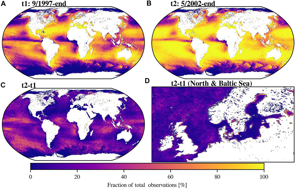
FIGURE 9. Data kept after applying the TGDM: (A) The fraction of observations of the full period, t1, and (B) the period t2 (5/2002–6/2020). In t2 the period when only SeaWiFS is active, is not included. Difference in data coverage between t1 and t2, globally (C) and in detail, its subset (D) for the Baltic-, North Sea, and surrounding sea.

If the first sub-period, observed by SeaWiFS only, is removed (t2: 5/2002–6/2020), the coverage density is greatly improved and the amount of data kept after applying the TGDM globally is 89%. The number of observations after applying the TGDM, has increased for all sensors, and slightly more gained observations originate from MERIS and OLCI (Table 4). The coverage density increases predominantly in high latitudes, areas with high cloud cover (Figure 9C), and near the coast (Figure 9D). These gained records were not included before because the SeaWiFS data set processed with l2gen, has smaller latitudinal range and a lesser ability to observe pixels near the coast. Therefore the first sub-period is the limiting factor when applying the TGDM to the full data set.

TABLE 4

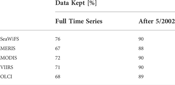
TABLE 4. The fraction of data kept after applying the TGDM for the two periods, separately shown for each sensor.

5 Discussion and Conclusion

The importance of temporal consistency in long-term time series cannot be stressed enough (GCOS, 2011). This study demonstrates that differences in data coverage of ocean colour satellite missions result in significant inter-mission inconsistencies in a merged data set. These inconsistencies appear as sudden steps when a satellite mission is introduced or terminated in the OC-CCI-v5 time series. We suspect that coverage discrepancies between sensors potentially affects multiple studies that use merged satellite data sets - in context with ocean colour, since similar patterns have been found earlier (e.g., Kahru et al., 2012, 2015; Navarro et al., 2017; Sankar et al., 2019; Kulk et al., 2020; Joseph et al., 2021). A novel method, the TGDM, is introduced that leads to a temporal homogenisation of observations per geographic pixel in the data set and effectively reduces the observed inter-mission inconsistencies in the time series. In our view, the results offer improved insights by enhancing the interpretation of merged data sets, and in particular that of ocean colour time series.

5.1 Coverage homogenization

Jackson (2020) suggests that inter-mission inconsistencies can be minimised by applying a logarithmic transformation to the data set. In effect, this approach reduces the contribution from areas consisting of relatively high Chl-a, making the global average approximately ∼30% lower. The Simc is reduced, but it remains significant after applying the logarithmic transformation to the OC-CCI-v5 Chl-a data set (Figure 1B) as the proposed approach does not account for differences in data coverage of the different satellite missions. The TGDM statistically removes irregularly observed records independent of the absolute values of the variable in focus. The optimal time window length in the TGDM is found when the Simc is insignificant, i.e., in the same order of magnitude as the noise of the time series. The length of the optimal time window also has a direct influence on how many data can be used for analysis. By using the optimal time window length of 27 days on the full data set, approximately 30% of daily records are masked globally. This may seem excessive, however, masking these (potentially high quality) records is necessary to create a temporally consistent time series that contains minimal inter-mission inconsistencies caused by irregular coverage. This is essential for a correct interpretation of long-term data analysis that includes data from different satellite missions.

5.2 Characteristics of the masked records

The first period (9/1997–4/2002) in the OC-CCI data set is solely observed by SeaWiFS. The global number of daily-averaged observations by SeaWiFS is lower than by the other ocean colour sensors because of the initially lower spatial resolution (4 km for SeaWiFS GAC vs. 1 km) and the additional flagging for invalidity of the atmospheric correction (l2gen). Consequently, it is the dominant factor in the TGDM as the observational gaps of SeaWiFS determine the records that are masked to a great degree. By excluding this first period, the coverage density after applying the TGDM is increased significantly (Figures 9C,D). Particularly in areas near the coast, with high cloud cover, and at high latitudes. The disadvantage is that the time series initiates ∼4.5 years later. The records masked with the TGDM are not of lower quality, but are excluded because they are not observed consistently over time in the merged data set due to the different coverage capabilities of the sensors. OLCI and MERIS have a relatively early local overpass time (10:00) compared to SeaWiFS (12:20), MODIS (13:30) and VIIRS (13:30). Clouds commonly develop during the day, thus sensors with a later overpass time may encounter more obscured pixels. Many observations are gained in generally cloudy areas when applying the TGDM to the time series without the SeaWiFS-only period (after 5/2002) when comparing the patterns of Figure 9C to the composite cloud coverage between 2001 and 2010 presented by Mercury et al. (2012). The lack of coverage during the SeaWiFS-only period in commonly cloudy areas, is caused by the overpass timing along with observing fewer pixels overall, since it was the only sensor operating during that time. It must be pointed out that changes in coverage over time may not solely be caused by the change of satellites, but possibly also by shifts and trends in global cloud coverage (Mao et al., 2019). Pixels at regions with high solar zenith angles are masked more frequently in the full time series because of differences in the Level-2 processing, i.e. the atmospheric correction. Pixels from highly-scattering waters, i.e., turbid waters, are also more often flagged for invalidity when conducting atmospheric correction with l2gen. This results in a lower contribution of SeaWiFS observations of bright pixels. These pixel exist, for example, near river mouths, and within blooms of coccolithophores. Calcite-producing coccolithophores are highly scattering single-celled organisms that are generally confined to temperate to subpolar waters in the upper part of the euphotic zone (Balch et al., 2018). MERIS and OLCI provide a better coastal coverage than the other satellite sensors present in the data set (Figure 6A). The global average of Chl-a is highest during the period when MERIS is active because it observes a greater number of pixels of high Chl-a, e.g., on productive, coastal shelves. This presents itself as sudden steps in a time series when the MERIS mission starts and ends. After applying the TGDM, the average Chl-a values near the coast have equalised for all sensors (Table 2). The highest latitudes observed in the full time series and in December have levelled as well for all sensors after applying TGDM (Figures 6E,F).

5.3 Temporal composition

On a daily basis, clouds, aerosols, inter-orbit gaps, Sun glint, and high solar zenith angles prevent complete daily coverage by either obscuration or lack of sampling. This irregular spatio-temporal sampling of ocean colour sensors can produce inconsistencies in monthly and annual mean Chl-a estimates (Gregg and Casey, 2007). Monthly composites have better data coverage, but daily and weekly processes cannot be resolved (Cole et al., 2012). Monthly composite time series are used extensively for analysing long-term trends, seasonal variability, and anomalies in ocean colour data sets (e.g., Henson et al., 2010; Djavidnia et al., 2010; Mélin, 2016; Hammond et al., 2018; Sankar et al., 2019; Gittings et al., 2021). They rely on a sub-sample of days, which may introduce uncertainty (IOCCG, 2019). Several studies have shown that statistics of inter-mission comparisons are degraded when comparing monthly averages concerning daily values, particularly when the number of days is relatively low (Barnes and Hu, 2015). Using monthly composites reduces differences due to noise, but also integrates differences created by irregular sampling by each sensor (Djavidnia et al., 2010). Monthly composites can be safely used after applying the TGDM because the irregular sampling inconsistency is minimised.

5.4 Consequences for phenology

The average daily coverage increases significantly by merging multiple ocean colour data sets (IOCCG, 2007; Maritorena et al., 2010). Caution is advised, when producing long-term statistics on this type of data, since the coverage is distributed unequally in both time and space. This has implications also for performing and interpreting phenology studies. The amount of missing data is directly related to the initiation, peak, and duration of an algal bloom (Cole et al., 2012; Racault et al., 2014). A greater amount of missing data records result in determining a later initiation and peak timing of a bloom, and a decreasing duration of a bloom. For example, the study by Kahru et al. (2011) found that in the Foxe Basin, Baffin Bay, and Kara Sea, the annual maximum Chl-a of the bloom to become seasonally earlier, and also of longer duration over the years. They used the merged GlobColour data set (SeaWiFS, MERIS, and MODIS). Our results here show that SeaWiFS coverage is poor in these areas (which are all located above the Arctic Circle) because the number of observations has increased significantly in these areas when the SeaWiFS-only period (9/1997–4/2002) is not included in the TGDM (Figure 9C). This means that the first period of the time series consists not only of fewer observations but also of seasonally, unequally observed pixels, compared to later years when the data sets from other satellites are added. SeaWiFS does not observe pixels as far north as other sensors. Thus, it may observe the spring bloom later, or not at all. For example, the study by Staehr et al. (2022), who used a merged data set consisting of the SeaWiFS, MODIS, MERIS, and VIIRS sensors in the Kattegat, found that the number of spring blooms are severely underestimated between 1998 and 2002, compared to the in situ data. Which is exactly the period when only SeaWiFS is active. In later years, the satellite data improved by matching the in situ data better. Gittings et al. (2021), who used the OC-CCI-v4 data set, found anomalies that seem to coincide with the presence of sensors as well, specifically when MERIS commences. During the period when MERIS is active, from 2002 to 2012, the spring bloom initiates earlier and terminates later in the Red Sea. The amount of observed data points increases after 2002, particularly in coastal waters when MERIS joins the data set. Our findings here suggest that these results may (partly) be artefacts due to the use of different satellite sensors, since the amount of missing data is directly related to bloom initiation and duration.

5.5 Recommendations

Merging ocean colour data sets is essential for ensuring continuity and consequently enabling the derivation of long-term statistics and trends. Our results demonstrate that inconsistencies in inter-mission coverage introduce significant artefacts in the time series of ocean colour products, which are not caused by a true change of the water surface leaving reflectance or poor correction of sensor sensitivities. Therefore, we recommend to temporally homogenise the coverage of merged data sets and presented a method (TGDM) to perform such a correction.

Future research is certainly required to investigate the effect of coverage differences between sensors in merged data sets on, e.g., trends regarding bloom initiation, peak and duration of a bloom. The TGDM homogenises the coverage of merged data sets and can therefore be used reliably for long-term phenology studies. One disadvantage of the TGDM is that areas of potentially high interest are partly masked out, which may lead to under-sampling for frequency analysis. Phenology studies generally profit from more observations–but only, if these are distributed equally over time. TGDM masks observations that are unequally distributed over time in the data set, and therefore reduces potentially biased trends. The coverage density can be improved considerably when the period before 5/2002 is excluded from the OC-CCI-v5 data set. Another approach that may be beneficial to phenology studies is decreasing the amount of missing data points. This can be achieved by, e.g., using weekly composites or decreasing the spatial resolution after applying a temporal homogenisation method, such as the TGDM.

The Simc, caused by inter-mission coverage differences, is smaller in the median and the logarithmically transformed Chl-a time series compared to the average Chl-a time series (Figures 1B, 8). Additionally, the Simc of the Chl-a time series is reduced by not including pixels located on the coastal shelf or at high latitudes. Therefore, using the median or the logarithmically transformed Chl-a as well as not including the coastal shelf or areas at high latitudes may reduce the Simc sufficiently for some type of studies, even without applying our method.

The TGDM is most useful in quantitative, large merged data sets where it is possible to mask just a few percent of the data set. A goal of this study is to construct a temporally consistent data set where the variable values (e.g., Chl-a) do not change because the inter-mission coverage changes. The TGDM masks irregularly observed pixels. To increase the number of observations when applying the TGDM, it may be useful to determine the optimal time window length per region. Areas with an initial insignificant Simc can likely be processed using a longer time window for the TGDM. This ensures that more data remains available. For example, many data records can be recovered south of the tropics because the initial Simc is not as pronounced there compared to north of the tropics (Figure 8). The initial Simc is smaller because this area consists of more pixels with relatively constant ocean colour properties. However, relative to the tropics and north of the tropics, more data are masked because of more persistent cloud cover. More research is needed to investigate these local differences to avoid unnecessary data loss.

For the production of merged ocean colour data sets, we recommend using a similar atmospheric correction for all sensor data, when possible. This ensures that pixels with similar ocean colour properties are flagged for invalidity in the data set. Areas that are inconsistently observed between sensors are unsuitable for in situ or virtual monitoring stations that aim to assess long-term trends or statistics because these can result in artefacts. Ideally, before setting up monitoring stations, the coverage differences between sensors should be evaluated for the location of the monitoring station. For existing monitoring stations, it is important to make sure that there are no coverage inconsistencies before drawing any long-term conclusions. If observational inconsistencies do exist, TGDM could be applied to correct for this. To ensure further continuity of the ocean colour Environmental Climate Data records and ability to analyse long-term time series, more satellite data sets should be added (e.g., Sentinel-3B) and new missions should be deployed to maintain sufficient overlap between data sets.

Surely, long-term analysis of satellite data based on several missions of varying sensor types, must consider the consequences of the differences in the capacity of different sensors to observe specific regions and times. Temporal coverage homogenisation is advised on this type of data to avoid introducing artefacts in long-term statistical analysis.

Data availability statement

The raw data supporting the conclusions of this article will be made available by the authors, without undue reservation.

Author contributions

All authors jointly developed the concept and work plan. MvO developed the TDGM method, all the calculations, preparation of figures, lead on writing the manuscript. All authors reviewed and provided comments on the draft manuscript and reviews.

Conflict of interest

The authors declare that the research was conducted in the absence of any commercial or financial relationships that could be construed as a potential conflict of interest.

Publisher’s note

All claims expressed in this article are solely those of the authors and do not necessarily represent those of their affiliated organizations, or those of the publisher, the editors and the reviewers. Any product that may be evaluated in this article, or claim that may be made by its manufacturer, is not guaranteed or endorsed by the publisher.

Acknowledgments

This work is a contribution to the Ocean Colour Climate Change Initiative of the European Space Agency and was supported by the Helmholtz Association within the Earth and Environment research program. We would like to thank Arnold G. Dekker and the OC-CCI team for their valuable input and discussions. Thanks also to Geoffrey Bonning for his helpful suggestions. Finally, we would like to thank the reviewers for taking the time and effort to review the manuscript.

References

Balch, W. M., Bowler, B. C., Drapeau, D. T., Lubelczyk, L. C., and Lyczkowski, E. (2018). Vertical distributions of coccolithophores, PIC, POC, biogenic silica, and chlorophyll a throughout the global ocean. Glob. Biogeochem. Cycles 32 (1), 2–17. doi:10.1002/2016GB005614

PubMed Abstract | CrossRef Full Text | Google Scholar

Barnes, B. B., and Hu, C. (2015). Cross-sensor continuity of satellite-derived water clarity in the gulf of Mexico : Insights into temporal aliasing and implications for long-term water clarity assessment. IEEE Trans. Geosci. Remote Sens. 53 (4), 1761–1772. doi:10.1109/TGRS.2014.2348713

CrossRef Full Text | Google Scholar

Brewin, R. J. W., Mélin, F., Sathyendranath, S., Steinmetz, F., Chuprin, A., and Grant, M. (2014). On the temporal consistency of chlorophyll products derived from three ocean-colour sensors. ISPRS J. Photogrammetry Remote Sens. 97, 171–184. doi:10.1016/j.isprsjprs.2014.08.013

CrossRef Full Text | Google Scholar

Campbell, J. W. (1995). The lognormal distribution as a model for bio-optical variability in the sea. J. Geophys. Res. 100 (C7), 13237. doi:10.1029/95jc00458

CrossRef Full Text | Google Scholar

Cleveland, R. B., Cleveland, W. S., McRae, J. E., and Terpenning, I. (1990). Stl: A seasonal-trend decomposition procedure based on loess. J. Official Statistics 6 (1), 3–73. doi:10.1007/978-1-4613-4499-5_24

CrossRef Full Text | Google Scholar

Cole, H., Henson, S., Martin, A., and Yool, A. (2012). Mind the gap : The impact of missing data on the calculation of phytoplankton phenology metrics. J. Geophys. Res. 117 (July), 2–9. doi:10.1029/2012JC008249

CrossRef Full Text | Google Scholar

Djavidnia, S., Mélin, F., and Hoepffner, N. (2010). Comparison of global ocean colour data records. Ocean. Sci. 6 (1), 61–76. doi:10.5194/os-6-61-2010

CrossRef Full Text | Google Scholar

Dutkiewicz, S., Monier, E., Hickman, A. E., Jahn, O., Henson, S., Beaulieu, C., et al. (2019). Ocean colour signature of climate change. Nat. Commun. 10 (1), 578. doi:10.1038/s41467-019-08457-x

PubMed Abstract | CrossRef Full Text | Google Scholar

Falkowski, P. G., and Raven, J. A. (2001). An introduction to photosynthesis. J. Phycol. 36 (2), 445–446. doi:10.1046/j.1529-8817.2000.99br2.x

CrossRef Full Text | Google Scholar

Field, C. B., Behrenfeld, M. J., Randerson, J. T., and Falkowski, P. (1998). Primary production of the biosphere : Integrating terrestrial and oceanic components. Science 281, 237–240. doi:10.1126/science.281.5374.237

PubMed Abstract | CrossRef Full Text | Google Scholar

Franz, B. A., Bailey, S. W., Werdell, P. J., and Mcclain, C. R. (2007). Sensor-independent approach to the vicarious calibration of satellite ocean color radiometry. Appl. Opt. 46 (22), 5068. doi:10.1364/AO.46.005068

PubMed Abstract | CrossRef Full Text | Google Scholar

Garnesson, P., Mangin, A., D’Andon, O. F., Demaria, J., and Bretagnon, M. (2019). The CMEMS GlobColour chlorophyll &lt;i&gt;a&lt;/i&gt; product based on satellite observation: Multi-sensor merging and flagging strategies. Ocean. Sci. 15 (3), 819–830. doi:10.5194/os-15-819-2019

CrossRef Full Text | Google Scholar

GCOS (2011). Systematic observation requirements for satellite-based products for climate 2011 update: Supplemental details to the satellite-based component of the “implementation plan for the global observing system for climate in support of the UNFCCC (2010 update). World meteorological organization. Available at: www.wmo.int/pages/prog/gcos/Publications/gcos-154.pdf.

Google Scholar

GCOS (2016). The global observing system for climate: Implementation needs. Available at: https://library.wmo.int/doc_num.php?explnum_id=3417.200138

Google Scholar

Gittings, J. A., Raitsos, D. E., Brewin, R. J. W., and Hoteit, I. (2021). Links between phenology of large phytoplankton and fisheries in the northern and central red sea. Remote Sens. 13 (2), 231. doi:10.3390/rs13020231

CrossRef Full Text | Google Scholar

Gregg, W. W., and Casey, N. W. (2010). Improving the consistency of ocean color data: A step toward climate data records. Geophys. Res. Lett. 37 (4), 1–5. doi:10.1029/2009GL041893

CrossRef Full Text | Google Scholar

Gregg, W. W., and Casey, N. W. (2007). Sampling biases in MODIS and SeaWiFS ocean chlorophyll data. Remote Sens. Environ. 111 (1), 25–35. doi:10.1016/j.rse.2007.03.008

CrossRef Full Text | Google Scholar

Groom, S., Sathyendranath, S., Jackson, T., Melin, F., Chuprin, A., Steinmetz, F., et al. (2022). the Ocean colour climate change initiative : Version 5 and preview of version 6. Living planet symposium 2022. Available at: climate.esa.int/media/documents/OC_CCI_poster_V5_V6a.pdf.

Google Scholar

Hammond, M. L., Beaulieu, C., Henson, S. A., and Sahu, S. K. (2018). Assessing the presence of discontinuities in the ocean color satellite record and their effects on chlorophyll trends and their uncertainties. Geophys. Res. Lett. 45 (15), 7654–7662. doi:10.1029/2017GL076928

CrossRef Full Text | Google Scholar

Harris, G. P. (1986). Phytoplankton ecology: Structure, function and fluctuation. 1st edn. Dordrecht: Springer. doi:10.1007/978-94-009-3165-7

CrossRef Full Text | Google Scholar

Henson, S. A., Sarmiento, J. L., Dunne, J. P., Bopp, L., Lima, I., Doney, S. C., et al. (2010). Detection of anthropogenic climate change in satellite records of ocean chlorophyll and productivity. Biogeosciences 7 (2), 621–640. doi:10.5194/bg-7-621-2010

CrossRef Full Text | Google Scholar

IOCCG (2000). Dartmouth in Remote sensing of ocean colour in coastal, and other optically-complex, waters. Editor S. Sathyendranath (Canada: International Ocean-Colour Coordinating Group), No. 3. doi:10.25607/OBP-95

CrossRef Full Text | Google Scholar

IOCCG (2007). International Ocean-Colour Coordinating Group in ocean-colour data merging. Editor W. W. Gregg (Canada: Dartmouth), No. 6. doi:10.25607/OBP-100

CrossRef Full Text | Google Scholar

IOCCG (2019). “,”. International Ocean-Colour Coordinating Group in Uncertainties in ocean colour remote sensing. Editor F. Mélin (Canada: Dartmouth), No 18. doi:10.25607/OBP-696

CrossRef Full Text | Google Scholar

Jackson, T. (2020). Product user guide for v5.0 dataset. D4.2. ESA. Available at: https://docs.pml.space/share/s/okB2fOuPT7Cj2r4C5sppDg.

Google Scholar

Jackson, T., Volpe, G., Sathyendranath, S., and Groom, S. (2021). Product validation and inter-comparison report. D4.1(1.0 ESA/ESRIN), pp. 1–17. Plymouth: Plymouth Marine Laboratory. Available at: https://docs.pml.space/share/s/xztLpM-NRka9rqoeSQFw5A.

Google Scholar

Joseph, D., Rojith, G., Zacharia, P. U., Sajna, V. H., Akash, S., and George, G. (2021). Spatio-temporal variations of chlorophyll from satellite derived data and CMIP5 models along Indian coastal regions. J. Earth Syst. Sci. 130 (153), 153. doi:10.1007/s12040-021-01663-6

CrossRef Full Text | Google Scholar

Kahru, M., Brotas, V., Manzano-Sarabia, M., and Mitchell, B. G. (2011). Are phytoplankton blooms occurring earlier in the Arctic? Glob. Change Biol. 17 (4), 1733–1739. doi:10.1111/j.1365-2486.2010.02312.x

CrossRef Full Text | Google Scholar

Kahru, M., Kudela, R. M., Manzano-Sarabia, M., and Greg Mitchell, B. (2012). Trends in the surface chlorophyll of the California Current: Merging data from multiple ocean color satellites. Deep-Sea Res. Part II Top. Stud. Oceanogr. 77–80, 89–98. doi:10.1016/j.dsr2.2012.04.007

PubMed Abstract | CrossRef Full Text | Google Scholar

Kahru, M., Lee, Z. P., Kudela, R. M., Manzano-Sarabia, M., and Greg Mitchell, B. (2015). Multi-satellite time series of inherent optical properties in the California Current. Deep-Sea Res. Part II Top. Stud. Oceanogr. 112, 91–106. doi:10.1016/j.dsr2.2013.07.023

CrossRef Full Text | Google Scholar

Kirk, J. T. O. (2011). Light and photosynthesis in aquatic ecosystems. 3rd edn. Cambridge, UK: Cambridge University Press. doi:10.1017/CBO9781139168212

CrossRef Full Text | Google Scholar

Kulk, G., Platt, T., Dingle, J., Jackson, T., Jönsson, B. F., Bouman, H., et al. (2020). Primary production, an index of climate change in the ocean: Satellite-based estimates over two decades. Remote Sens. 12 (5), 826. doi:10.3390/rs12050826

CrossRef Full Text | Google Scholar

Lee, Z. P., Darecki, M., Carder, K. L., Davis, C. O., Stramski, D., Rhea, W. J., et al. (2005). Diffuse attenuation coefficient of downwelling irradiance: An evaluation of remote sensing methods. J. Geophys. Res. 110 (2), C02017. doi:10.1029/2004JC002573

CrossRef Full Text | Google Scholar

Lee, Z. P., Lubac, B., Werdell, J., and Arnone, R. (2009). ‘An update of the quasi-analytical algorithm (QAA_v5)’, technical report, international ocean colour coordinating group (IOCCG). Available at: http://www.ioccg.org/groups/software.html.

Google Scholar

Mao, K., Yuan, Z., Zuo, Z., Xu, T., Shen, X., and Gao, C. (2019). Changes in global cloud cover based on remote sensing data from 2003 to 2012. Chin. Geogr. Sci. 29 (2), 306–315. doi:10.1007/s11769-019-1030-6

CrossRef Full Text | Google Scholar

Maritorena, S., D’Andon, O. H. F., Mangin, A., and Siegel, D. A. (2010). Merged satellite ocean color data products using a bio-optical model: Characteristics, benefits and issues. Remote Sens. Environ. 114 (8), 1791–1804. doi:10.1016/j.rse.2010.04.002

CrossRef Full Text | Google Scholar

Mélin, F., Chuprin, A., Grant, M., Jackson, T., and Sathyendranath, S. (2016). ‘ocean colour data bias correction and merging’. ESA, 9-25. Available at: https://docs.pml.space/share/s/2RVhiuK2SWyhbSthqDDoxg.

Google Scholar

Mélin, F. (2016). Impact of inter-mission differences and drifts on chlorophyll-a trend estimates. Int. J. Remote Sens. 37 (10), 2233–2251. doi:10.1080/01431161.2016.1168949

CrossRef Full Text | Google Scholar

Mélin, F., and Sclep, G. (2015). Band shifting for ocean color multi-spectral reflectance data. Opt. Express 23 (3), 2262. doi:10.1364/oe.23.002262

PubMed Abstract | CrossRef Full Text | Google Scholar

Mélin, F., Vantrepotte, V., Chuprin, A., Grant, M., Jackson, T., and Sathyendranath, S. (2017). Assessing the fitness-for-purpose of satellite multi-mission ocean color climate data records: A protocol applied to OC-CCI chlorophyll- a data. Remote Sens. Environ. 203, 139–151. doi:10.1016/j.rse.2017.03.039

PubMed Abstract | CrossRef Full Text | Google Scholar

Mercury, M., Green, R., Hook, S., Oaida, B., Wu, W., Gunderson, A., et al. (2012). Global cloud cover for assessment of optical satellite observation opportunities: A HyspIRI case study. Remote Sens. Environ. 126, 62–71. doi:10.1016/j.rse.2012.08.007

CrossRef Full Text | Google Scholar

Moore, T. S., Campbell, J. W., and Dowell, M. D. (2009). A class-based approach to characterizing and mapping the uncertainty of the MODIS ocean chlorophyll product. Remote Sens. Environ. 113 (11), 2424–2430. doi:10.1016/j.rse.2009.07.016

CrossRef Full Text | Google Scholar

Moss, B. R. (2009). Ecology of fresh waters: Man and medium, past to future. 3rd edn. John Wiley & Sons.

Google Scholar

Müller, D., Krasemann, H., Brewin, R. J. W., Brockmann, C., Deschamps, P., Doerffer, R., et al. (2015a). Remote sensing of environment the Ocean colour climate change initiative : II . Spatial and temporal homogeneity of satellite data retrieval due to systematic effects in atmospheric correction processors. Remote Sens. Environ. 162, 257–270. doi:10.1016/j.rse.2015.01.033

CrossRef Full Text | Google Scholar

Müller, D., Krasemann, H., Brewin, R. J. W., Brockmann, C., Deschamps, P. Y., Doerffer, R., et al. (2015b). the Ocean colour climate change initiative: I. A methodology for assessing atmospheric correction processors based on in-situ measurements. Remote Sens. Environ. 162 (April), 242–256. doi:10.1016/j.rse.2013.11.026

CrossRef Full Text | Google Scholar

Navarro, G., Almaraz, P., Caballero, I., Vázquez, Á., and Huertas, I. E. (2017). Reproduction of spatio-temporal patterns of major mediterranean phytoplankton groups from remote sensing OC-CCI data. Front. Mar. Sci. 4 (AUG), 1–16. doi:10.3389/fmars.2017.00246

CrossRef Full Text | Google Scholar

Racault, M.-F., Sathyendranath, S., and Platt, T. (2014). Impact of missing data on the estimation of ecological indicators from satellite ocean-colour time-series. Remote Sens. Environ. 152, 15–28. doi:10.1016/j.rse.2014.05.016

CrossRef Full Text | Google Scholar

Sankar, S., Ramachandran, A. T., Ghomsi, K., Eitel, F., Kondrik, D., Sen, R., et al. (2019). The influence of tropical Indian Ocean warming and Indian Ocean Dipole on the surface chlorophyll concentration in the eastern Arabian Sea. Biogeosciences Discuss., 1–23. (June). doi:10.5194/bg-2019-169

CrossRef Full Text | Google Scholar

Sathyendranath, S., Brewin, R. J. W., Brockmann, C., Brotas, V., Calton, B., Chuprin, A., et al. (2019). An ocean-colour time series for use in climate studies: The experience of the ocean-colour climate change initiative (OC-CCI). Sensors 19 (19), 4285. doi:10.3390/s19194285

CrossRef Full Text | Google Scholar

Sathyendranath, S., Brewin, R. J. W., Jackson, T., Mélin, F., and Platt, T. (2017). Ocean-colour products for climate-change studies: What are their ideal characteristics? Remote Sens. Environ. 203, 125–138. doi:10.1016/j.rse.2017.04.017

CrossRef Full Text | Google Scholar

Sathyendranath, S., Jackson, T., Brockmann, C., Brotas, V., Calton, B., Chuprin, A., et al. (2021). ESA ocean colour climate change initiative (Ocean_Colour_cci): Version 5.0 data. NERC EDS Centre for Environmental Data Analysis. doi:10.5285/1dbe7a109c0244aaad713e078fd3059a

CrossRef Full Text | Google Scholar

Staehr, S. U., Van der Zande, D., Staehr, P. A. U., and Markager, S. (2022). Suitability of multisensory satellites for long-term chlorophyll assessment in coastal waters: A case study in optically-complex waters of the temperate region. Ecol. Indic. 134, 1–12. December 2021. doi:10.1016/j.ecolind.2021.108479

CrossRef Full Text | Google Scholar

Steinmetz, F., Deschamps, P.-Y., and Ramon, D. (2011). Atmospheric correction in presence of sun glint: Application to MERIS. Opt. Express 19 (10), 9783. doi:10.1364/oe.19.009783

PubMed Abstract | CrossRef Full Text | Google Scholar

Steinmetz, F., Ramon, D., and Deschamps, P.-Y. (2016). ATBD v1 - polymer atmospheric correction algorithm. ESA. Available at: https://docs.pml.space/share/s/M05k8Lw3QLeXSIiA3X87UQ.

Google Scholar

Valente, A., Sathyendranath, S., Brotas, V., Groom, S., Grant, M., Taberner, M., et al. (2019). A compilation of global bio-optical in situ data for ocean-colour satellite applications - version two. Earth Syst. Sci. Data. Copernicus Publications. doi:10.5194/essd-11-1037-2019

CrossRef Full Text | Google Scholar