QWIP: A Quantitative Metric for Quality Control of Aquatic Reflectance Spectral Shape Using the Apparent Visible Wavelength

The colors of the ocean and inland waters span clear blue to turbid brown, and the corresponding spectral shapes of the water-leaving signal are diverse depending on the various types and concentrations of phytoplankton, sediment, detritus and colored dissolved organic matter. Here we present a simple metric developed from a global dataset spanning blue, green and brown water types to assess the quality of a measured or derived aquatic spectrum. The Quality Water Index Polynomial (QWIP) is founded on the Apparent Visible Wavelength (AVW), a one-dimensional geophysical metric of color that is inherently correlated to spectral shape calculated as a weighted harmonic mean across visible wavelengths. The QWIP represents a polynomial relationship between the hyperspectral AVW and a Normalized Difference Index (NDI) using red and green wavelengths. The QWIP score represents the difference between a spectrum’s AVW and NDI and the QWIP polynomial. The approach is tested extensively with both raw and quality controlled field data to identify spectra that fall outside the general trends observed in aquatic optics. For example, QWIP scores less than or greater than 0.2 would fail an initial screening and be subject to additional quality control. Common outliers tend to have spectral features related to: 1) incorrect removal of surface reflected skylight or 2) optically shallow water. The approach was applied to hyperspectral imagery from the Hyperspectral Imager for the Coastal Ocean (HICO), as well as to multispectral imagery from the Visual Infrared Imaging Radiometer Suite (VIIRS) using sensor-specific extrapolations to approximate AVW. This simple approach can be rapidly implemented in ocean color processing chains to provide a level of uncertainty about a measured or retrieved spectrum and flag questionable or unusual spectra for further analysis.

1 Introduction

The color of a water body is a complex mixture of light that has been reflected from the water surface (sky and other floating substances) and reflected from within the water column (water color). The aquatic optics community refers to the water color reflectance as “Water-leaving Radiance Reflectance” (R_w) or more commonly, but less descriptively, “Remote Sensing Reflectance” (R_rs). Many methods are available to estimate R_rs both from instruments within and above the water surface and from aircraft and satellites orbiting the Earth. Each method to approximate R_rs involves some level of estimation to either remove the specular reflectance from the air-water interface from the above water measurement or to propagate the underwater upwelling signal to and across the interface, as well as to compensate for instrument shading and other measurement artifacts (Ruddick et al., 2019; Zibordi et al., 2019; Lee et al., 2020). To meet the needs of a growing list of applications for water color imagery (Dierssen et al., 2021), more automated data analysis is essential to develop and validate different approaches to assess regional and global aquatic optical properties and phytoplankton and benthic biodiversity. Automated systems are being developed to estimate R_rs from drones, moorings, profilers, and offshore platforms (summarized in Dierssen et al., 2020). As systems become more automated going forward and more “big data” hyperspectral datasets are generated routinely for use by the broader science community, new metrics are needed to provide automated quality control of data from different water types, as well as to assess the quality of satellite-retrievals of R_rs.

1.1 How Can I Assess the Data Quality of a Water Spectrum?

This simple sounding question is quite complex to answer objectively because R_rs is a derived parameter and the uncertainties are quite challenging to quantify for each method under a wide array of environmental conditions. Spectra are not only influenced by the optical properties of a large diversity of dissolved and particulate components and the potential contribution from the benthos, but also by measurement artifacts related to the solar and viewing angles, sky and wave conditions, air−water interface, platform disturbance, spatial inhomogeneity in the water column, and distance from land masses (Voss et al., 2017; Bulgarelli and Zibordi, 2020; Shang et al., 2020). If we screen out field data to encompass only a set of predefined or “ideal” conditions with calm seas, clear skies, and constrained solar and viewing angles, for example, then the measurement uncertainty is decreased significantly. This can be justified for the generation of fiducial reference spectra for satellite valiation and calibration, such as data from the Aeronet-OC program (Zibordi et al., 2009). However, as noted by a recent intercomparison exercise, there can still be considerable uncertainty in R_rs even under ideal conditions and with well-calibrated sensors (Tilstone et al., 2020). Moreover, such ideal conditions are rarely met in the field and represent only a fraction of the diverse environmental conditions encountered in natural ecosystems across latitudes and seasons. Retrieval models applied to satellite imagery also contain a much broader set of conditions, in terms of water column, atmosphere and surface states, as well as observation and illumination geometries. As retrieval approaches are diversifying, the community is finding that even non-optimal spectral information can still be useful for algorithm development and parameter validation for a variety of applications. For example, algorithms with narrowband indices or relying on derivatives may be less influenced by surface reflected sunlight than full inversion-type algorithms (Dierssen et al., 2021).

Many standard options are available for processing radiometric data, including flags for low solar zenith angles and low light conditions and for identifying rain, outlined in processing software such as HyperInSpace (Aurin, 2022). Operationally, site-specific criteria and thresholds are often developed based on careful examination of the data from that region. For example, spurious ship-based radiometric data were identified using five different spectral shape metrics tuned for highly absorbing and weakly scattering conditions characteristic of the Baltic Sea (Qin et al., 2017). The thresholds in such metrics are set based on human evaluation and interpretation of the expected data for a region.

1.2 Does My Water Spectrum Look Like Other Spectra?

For many aquatic data, there are clear standards that can be used to assess the quality of data. Such metrics are still being defined in the aquatic optics community due to the large range in environmental conditions and the many corrections that must be considered for any measurement (e.g., most absorption measurements have an associated scattering correction and most scattering measurements have an associated absorption correction). Commonly, intercomparisons between instruments and methods are the primary means to assess the operational uncertainties (Tilstone et al., 2020) or through simulation and closure studies (Zaneveld, 1994; Tzortziou et al., 2006), although assessing the accuracy of a measurement still remains an outstanding problem (Ruddick et al., 2019; Zibordi et al., 2019). In this paper we do not assess the accuracy of R_rs, but rather develop a method to assess the quality of a water spectrum using data collected and filtered using community standard practices.

Experienced researchers tend to have a “gut” sense for what looks like a reasonable spectrum, but definitive approaches for assessing spectral shape are limited. Questionable spectral shapes are readily identifiable when reflectance values in the near-infrared wavelengths are much higher than anticipated for the type of water collected or when spectra exhibit an exponentially increasing tail from blue to ultraviolet, indicating that reflected diffuse skylight may not be removed fully from the spectrum (Mobley, 1999; Gould et al., 2001). A recent work by Wei et al. (2016) provides a means of scoring a spectrum compared to 23 different simulated optical water types at a maximum of nine wavebands (Wei et al., 2016). This spectral matching approach provides a score as to how close a spectrum matches one of the predefined water types. As noted below, this approach may be limited to standard simulated conditions and may not represent all water types encountered across the vast aquascape (Barnes et al., 2019).

1.3 Are There Other Simple Metrics That Can be Used to Assess the Quality of a Water Spectrum?

Here, we present a simple quantitative index approach to conduct quality control of an R_rs spectrum and thereby determine whether it appears similar to other ocean color spectra from a wide variety of blue, green and brown water types. The Quality Water Index Polynomial (QWIP) is founded on the Apparent Visible Wavelength (AVW) a one-dimensional geophysical metric of “color,” calculated as the weighted harmonic mean of the reflectance spectrum across a range of wavelengths (Vandermeulen et al., 2020). This metric reduces the hyperspectral or multispectral (after applying sensor-specific correction factors) data to a continuous variable representing the mean “color” in wavelength (expressed in nm). As noted in Figure 10B of Vandermeulen et al. (2020), a good correlation is found between AVW and chlorophyll a concentrations using a global dataset. Building upon this, we developed a relationship between AVW and standard multi-channel waveband indices to identify spectra that fall outside the general trends observed in aquatic optics for optically deep waters. The approach was developed with a large global dataset representing blue, green, and brown waters and was further tested extensively with field and satellite datasets. This simple approach can be rapidly implemented in ocean color processing chains to provide a level of uncertainty about the spectrum and flag questionable or unusual spectra for further analysis.

2 Methods

The method was developed using a large global dataset of remote sensing reflectance compiled from different studies (CASCK-P dataset) and then tested using several different regional field datasets collected with above-water methodology and on satellite-retrievals of water-leaving reflectance data.

2.1 Field Datasets

2.1.1 CASCK Dataset (Casey, Castagna, and Knaeps)

The majority of the training dataset was obtained from a recent global compilation of hyperspectral optical data that includes profiled and buoy mounted in-water radiometers, as well as ship-mounted and hand-held above-water methods (Casey et al., 2020). Because intense green and brown water spectra are underrepresented in this dataset, we have augmented it with two additional coastal and inland water datasets. As such, a dataset comprised primarily of green water spectra with pronounced red edge reflectance, collected with a hand-held single spectrometer using the skylight-blocked method in nine different Belgian lakes and a lagoon, was included (Castagna et al., 2020). Above-water spectra of brown water from the Scheldt River Delta were also included (Castagna et al., submitted). An additional dataset collected with a hand-held single radiometer system in the river deltas of the Scheldt (Belgium), Gironde (France), and Río de la Plata (Argentina) with total suspended matter up to 1,400 g m⁻³ was also incorporated to represent extremely turbid conditions (Knaeps et al., 2015). In total, the CASCK dataset contains 1,029 R_rs spectra, and is provided in the Suplementary Material. The global distribution of the CASCK dataset is shown in Figure 1.

FIGURE 1

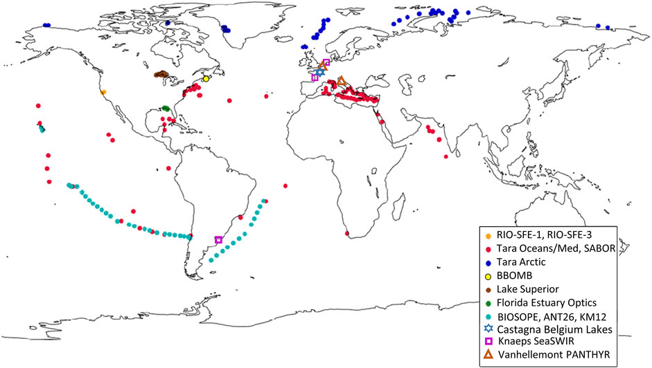
FIGURE 1. Sampling locations from the global hyperspectral training data (CASCK-P) used to develop the polynomial spanned open ocean, coastal, and inland waters. Adapted from Casey et al. (2020).

2.1.2 PANTHYR Venice and Ostend Datasets

Data from two autonomous hyperspectral PANTHYR radiometer systems (Vansteenwegen et al., 2019) deployed in the Adriatic Sea at the Acqua Alta Oceanographic Tower in the Gulf of Venice, Italy (AAOT, 45.3139°N, 12.5083°E) (n = 1,622) and in the North Sea at Research Tower 1 near Ostend, Belgium (RT1, 51.2464°N, 2.9193°E) (n = 4,945) from September to December 2019 were also included (Vanhellemont, 2020). The locations of the two towers is shown in Figure 1. These data were subject to considerable quality control and assessment including removing spectra collected under sub-optimal conditions as described in Vanhellemont (2020). A data paper further describing these data in final format is forthcoming.

2.1.3 WISP-3 Raw Dataset

Above-water data have been collected using the hand-held WISP-3 measurements as part of the Belgian coast Lifewatch program since April 2019 (Mortelmans et al., 2019). For this analysis, no quality assessment criteria were applied and the dataset included all training measurements including spectra taken of land, on deck, and with lens cap on in order to test the QWIP on wide array of good and bad spectra (n = 869). The instrument has three hyperspectral radiometers that simultaneously capture the downwelling plane irradiance, E_d, upwelling water system (surface + water-leaving) radiance (L_ws), and skylight radiance (L_sky) (Hommersom et al., 2012) The data were processed to remote sensing reflectance R_rs using a solar-zenith angle dependent ρ factor to account for spectral sea surface reflectance of skylight (Zhang et al., 2017). The ρ factor was calculated for a viewing angle of 40° to water, 135° azimuth from sun with an Aerosol Optical Thickness at 555 nm of 0.1. For these data, a wind speed of 5 m s⁻¹ was used and data collected under solar zenith angles greater than 60°, outside the scope of typical values, used a ρ comparable to SZA of 60°. Mean visible ρ used here ranged from 0.032 to 0.036. Residual skylight was removed with a baseline subtraction following a semi-analytical correction using two narrow band features in the near-infrared red at 715 and 735 nm following Gould et al. (2001). A spectrally flat residual baseline correction, B, was estimated from the measurements of radiance reflectance of skylight (R_sky = L_sky/E_d) and of the water system including water-leaving and surface reflected signal (R_ws=L_ws/E_d) according to:

$B=R_{\text{ws}}\left(735\right)-\rho \left(735\right) R_{\text{sky}}\left(735\right)-\frac{R_{\text{ws}}\left(715\right)-R_{\text{ws}}\left(735\right)}{\left(\frac{a_{\text{w}}\left(735\right)}{a_{\text{w}}\left(715\right)}-1\right)}(1)$

This correction assumes that absorption at 715 and 735 nm is dominated by pure water (a_w) and that the combined effects of backscattering, b_b, and the f/Q bidirectional factor, and residual skylight are well approximated by a spectrally flat value (equivalent in magnitude) between 715 and 735 nm. It is further assumed that the residual skylight signal is well approximated by B in the visible range. The assumption of spectrally flat pattern of b_b and f/Q is this narrow range is well justified (cf. Ruddick et al., 2006). The absorption by pure water at 715 and 735 nm were set at 1.0242 and 2.2780 m⁻¹, respectively (Röttgers et al., 2016).

2.2 Satellite Datasets

2.2.1 Hyperspectral Imager for the Coastal Ocean Dataset

We tested the proposed radiometric quality control procedure on a series of retrieved scenes from the Hyperspectral Imager for the Coastal Ocean (HICO), in order to examine the algorithm’s efficacy in the identification of low-quality satellite returns. HICO Level-1B files were downloaded from the NASA Ocean Biology Processing Group (https://oceancolor.gsfc.nasa.gov/l2), and processed using l2gen program packaged as part of the NASA SeaDAS (Ocean Biology Processing Group, 2022). A heritage atmospheric correction procedure was used (Gordon and Wang 1994; Bailey et al., 2010), with the additional use of the ATmospheric REMoval code (ATREM; Gao and Davis, 1997) built into l2gen, which provides hyperspectral compensation of the water vapor absorption for the atmospheric correction process, following Ibrahim et al. (2018). Data were processed to output a pixel-wise continuous spectra of R_rs from 398 to 702 nm, including all standard SeaDAS Level-2 flags. This includes the default masking threshold in l2gen that can exclude the most turbid waters. The AVW (Eq. 2) over the range of 400–700 nm was subsequently calculated for every pixel after interpolation of the spectrum to 1 nm resolution using cubic splines.

2.2.2 Visual Infrared Imaging Radiometer Suite Matchup Dataset

In an effort to examine the impact of applying automated quality control criteria on a multi-spectral validation stream, we retrieved all R_rs validation matchups for the Visual Infrared Imaging Radiometer Suite (SNPP-VIIRS) from the SeaWiFS Bio-optical Archive and Storage System (SeaBASS; https://seabass.gsfc.nasa.gov/search#val), for all SeaBASS and AERONET matchups (n = 2,850). The exclusion criteria followed NASA processing recommendations (Bailey and Werdell, 2006). An empirical conversion of the multispectral AVW values to a hyperspectral-equivalent AVW was applied to the VIIRS satellite and in situ matchups prior to analysis (Vandermeulen et al., 2020; Vandermeulen, 2022).

2.3 Water Color Classification

A simple decision tree was implemented to determine whether the spectral shape of R_rs would be classified as blue-green, green, or brown in color following from the approach presented in (Balasubramanian et al., 2020). This simplified classification (Figure 2) was used to indicate where different types of waters fall within the QWIP schema.

FIGURE 2

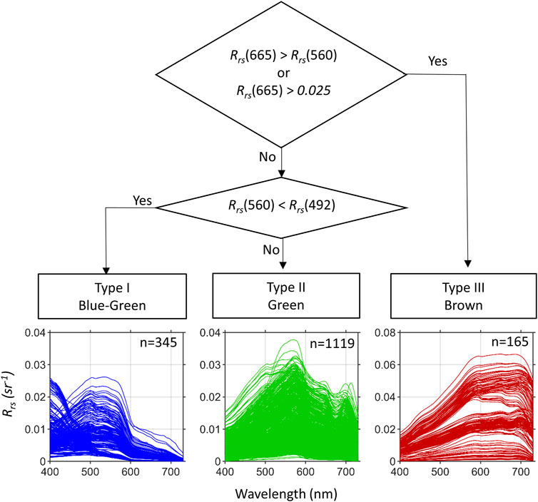
FIGURE 2. A simple screening approach modified from Balasubramanian et al. (2020) was used to evaluate the QWIP approach for three water types: Blue-green, Green, and Brown. The remote sensing spectra shown are from the (CASCK-P) training dataset and are identified with color and shape in Figures 3, 4 based on this schema.

2.4 Wei Score

Quality of all spectra was assessed according to the Wei et al. (2016) approach, using the Matlab-based code provided therein. Specifically, a multispectral subset was extracted for each spectrum (at wavelengths (nm): 412, 443, 488, 510, 531, 547, 555, 667, and 678), which was then normalized and compared to each of 23 reference spectra representing disparate optical water types. A spectral angle mapper was used to identify the most spectrally similar reference spectrum. Normalized reflectance data at each wavelength of the subset were then compared to the corresponding reference spectrum and associated boundaries. The final QA score was determined as the number wavelengths for which the reflectance datum fit within the reference boundaries, divided by the total number of wavelengths assessed (nine for this work). Thus QA scores ranged from 0 (at no wavelength does the target spectrum fit within boundaries of the identified water type) to 1 (target spectrum is fully within identified water type boundaries). Wei et al. (2016) qualitatively discusses “very high scores (>0.9)” and “very low QA scores (<0.5),” and reports that 90% of the evaluation spectra had “high QA scores” of >0.8. Based on this, a Wei score of >0.5 was considered as “Passing” and ≤0.5 was considered “Failing.”

2.5 Statistical Analyses

The equations used in the QWIP calculation include the Apparent Visible Wavelength (AVW) calculated from 400 to 700 nm at 1 nm intervals and the Normalized Difference Index (NDI) at two wavelengths as formulated below. Any negative values of R_rs are included in the calculations. We note that the QWIP and NDI acronyms are used in the equations below for clarity, such that:

$AVW=\left(\frac{{{\displaystyle \sum }}_{i=1}^n{R}_{\text{r}\text{s}}\left({\lambda }_i\right)}{{{\displaystyle \sum }}_{i=1}^n\frac{R_{\text{r}\text{s}}\left({\lambda }_i\right)}{{\lambda }_i}}\right)(2)$

$NDI= \frac{\left(R_{\text{r}\text{s}}\left({\lambda }_2\right)-R_{\text{r}\text{s}}\left({\lambda }_1\right)\right)}{\left(R_{\text{r}\text{s}}\left({\lambda }_2\right)+R_{\text{r}\text{s}}\left({\lambda }_1\right)\right)}(3)$

Statistical tests were conducted in Matlab (The Mathworks, Inc.). Model II regression analysis was used presuming similar uncertainty magnitudes in the involved variables.

2.6 Quality Water Index Polynomial Development

The algorithm is first developed using a global dataset covering a diverse set of (mostly) optically deep water types. A training dataset was compiled (n = 1,629) that included the CASCK data (see Supplemental Material) and 300 random points selected from each of the PANTHYR datasets, dubbed here the “CASCK-P” dataset (see Figure 1). We evaluated the relationships between AVW (the mean “color” metric, Eq. 2) and other indices to find trends across the wide range of spectral shapes in the dataset. The objective was to find a simple metric using common spectral bands found in a variety of multi-spectral datasets (i.e., wavebands from the VIIRS sensor wavelengths were selected here) where the central tendency of data formed a well-described continuum across the wide range of AVW values and the amount of deviations from the central tendency could be easily scored. To better visualize the data trends, the water color was further differentiated into the categories of blue-green (blue dots), green (green dots), and brown (red dots) following from the decision tree (see Figure 2). Blue-green waters have AVW values ranging from 400 to 510 nm and green waters have AVW from 510 to 590 nm. The AVW for brown waters overlaps with the upper end of the green waters, ranging from 555 to 575 nm.

The QWIP is formally a mathematical model relating an optical index to the AVW. Different examples of the relationships between AVW and other indices are provided in Figure 3 for illustrative purposes. Blue-to-green band ratios, like those used in chlorophyll algorithms and Vandermeulen et al. (2020), showed a reasonable overall trend, but resulted in the values being spread across a log scale with clustering of the green and red spectra (e.g., Figure 3A). Band difference algorithms provided lower predictive power, especially for the brown waters which had much higher differences than the blue and green waters (Figure 3B). Relationships between AVW and maximum wavelength in visible wavelengths (data not shown) were effective for blue and green waters, but proved to have low predictive power for intense green algal blooms with high red edge values and turbid brown waters. Brown waters can have variable peak wavelengths from green to red to near infrared wavelengths (see Figure 2).

FIGURE 3

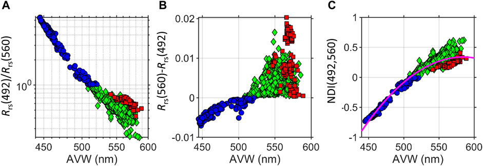
FIGURE 3. Examples of different spectral band math approaches compared to Apparent Visible Wavelength (AVW) evaluated with the CASCK-P training dataset separated by water type: Blue-green (blue circles), Green (green diamonds) and Brown (red squares). Approaches include (A) Band ratios (B) Band differences and (C) Normalized Difference Indices (NDIs) with different band combinations. These approaches were not selected for use due to overall fit and divergence of data from different water types.

The NDI (Eq. 3) provided a means to highlight the variability of logarithmically distributed data on a linear scale such that the distance either above or below the central tendency was scored with a positive or negative value. Different combinations of NDI were systematically evaluated using wavebands found on historic ocean color sensors. For example, the wavebands used in the standard chlorophyll a concentration algorithm (492 and 560 nm) (O’Reilly et al., 1998) did not have high rank correlation with the AVW for green and brown waters (Figure 3C). The best relationship was found using the NDI calculated with blue/green (λ₁ = 492 nm) and red (λ₂ = 665 nm) bands (Figure 4A). A 4th degree polynomial fit between NDI (492,665) and AVW described the variability across the AVW range (R² = 0.974). This QWIP relationship followed the overall objectives in that the central tendency was clearly outlined across a wide range of data and distance was easily scored. To implement, the user would calculate their AVW and NDI (492,665) for a spectrum following from Eqs. 2, 3 and then calculate the QWIP Score as the difference between the measured and the predicted NDI based on the QWIP. Note that the acronyms NDI, AVW, and QWIP are used in the equations below for clarity and the five coefficients in Eq. 4 correspond to five variables p provided below the equation:

$\begin{array}{l}\text{QWIP}=p_1{\text{AVW}}^4+p_2{\text{AVW}}^3+p_3{\text{AVW}}^2+p_4\text{AVW}+p_5\\ p=(-8.399885x{10}^{-9}, 1.715532x{10}^{-5},-1.301670x{10}^{-2},4.357838x{10}^0,-5.449532x{10}^2)\end{array}(4)$

$\text{QWIP score}=\text{NDI}\left(\mathrm{492,665}\right)-\text{QWIP}(5)$

FIGURE 4

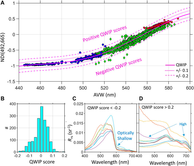
FIGURE 4. (A) The QWIP relationship between Apparent Visible Wavelength (AVW) and the Normalized Difference Index (NDI) with the CASCK-P training dataset showing the final tuned QWIP polynomial (thick magenta line) with different levels of QWIP scores (±0.1 dotted magenta and ±0.2 dashed magenta). Water types include: Blue-green (blue circles), Green (green diamonds) and Brown (red squares). (B) Histogram of the QWIP scores from (A) are predominantly within ±0.1 for the training data. (C) The remote sensing reflectance (R_rs) of outliers with negative QWIP scores < −0.2 were associated with optically shallow water features. (D) Outliers with QWIP scores > 0.2 exhibited higher blue associated with surface reflected skylight and higher overall magnitude spectra.

As shown in Figure 4A, 97.5% of the CASCK-P data used in the calibration of the QWIP fell within ± 0.1 of the QWIP and 99.4% within ± 0.2 (Figure 4B). Outlier data with QWIP scores greater than ± 0.2 were subject to additional screening to determine any evident spectral anomalies. The points with more negative QWIP scores (Figure 4C) appeared to be related to some types of optically shallow water where the red wavelengths were much lower than anticipated for highly green peaked waters due to water absorption between the scattering seafloor and the sea surface (e.g., Dierssen et al., 2003) suggesting the QWIP score may prove a useful metric for identifying certain types of optically shallow water. Data with high positive QWIP scores often had rising tails in the blue end of the spectrum consistent with data containing residual surface reflected skylight (Gould et al., 2001) (Figure 4C). In such cases, the AVW would be weighted incorrectly towards the blue end of the spectrum resulting in a positive QWIP score.

3 Results

The algorithm is evaluated on two different field datasets collected with above water methodology and two different satellite datasets (HICO and VIIRS).

3.1 Quality Water Index Polynomial Applied to Field Datasets

QWIP scores were calculated for two different above water field datasets for evaluation across a variety of water types with different instruments.

3.1.1 Quality-Controlled Data

The QWIP approach was tested on a highly calibrated above-water dataset collected from two different moorings (PANTHYR) (Vansteenwegen et al., 2019; Vanhellemont, 2020). The Ostend dataset (n = 1,622) contained primarily water that clustered as the water type 16 from Wei et al. (2016) with a strongly green-peaked spectral shape with a fluorescence/red edge characteristic of high phytoplankton. In contrast, the PANTHYR Aqua Alta dataset (n = 4,945) contained primarily water that ranged from Wei et al. (2016) types 6–10 with a high dynamic spectral range, more rounded blue/green spectral shape and very little fluorescence/red edge features. The mean QWIP score was 0.0135 with a small standard deviation of only 0.03 indicating that the data closely followed the mean tendency of the QWIP polynomial (Figures 5A,B). Over 98.7% of the data had a QWIP score within ± 0.1 and 100% within ± 0.2. With a maximum magnitude of |0.13|.

FIGURE 5

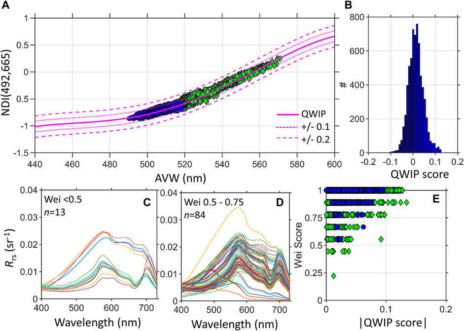
FIGURE 5. (A) The QWIP scores from highly quality controlled hyperspectral PANTHYR reflectance data from Vanhellemont (2020). (B) QWIP scores were predominantly within <± 0.1. Water types include: Blue-green (blue circles), Green (green diamonds) and Brown (red squares). Remote sensing reflectance of data with Wei scores (C) less than 0.5 (D) between 0.5 and 0.75. (E) Comparison of Wei scores (Wei et al., 2016) and the absolute value of QWIP scores for the entire dataset.

When compared to the spectral quality score proposed by Wei et al. (2016) (“Wei score”), the Wei score for the blue-green data of Aqua Alta were all >0.7 with a mean Wei score of 0.99. However, the Wei score predicted lower values for the more green-peaked water types of Ostend with a mean score of 0.93. Although all spectra passed QWIP, there were 13 spectra deemed failing with Wei scores <0.5 (Figure 5C) and 84 spectra of lower quality with Wei Scores of 0.5–0.75 (Figure 5D). The relationship between QWIP and Wei Score was not linear and did not follow the negative trend predicted by each method (Figure 5E), likely because of the use of only a select number of predefined water types using multi-spectral information in the Wei method, but both methods passed 99.8% of the spectra.

3.1.2 Raw WISP-3 Data

In addition to highly quality controlled data, we assessed how well the QWIP method would identify outliers in a raw dataset that included measurements made with the lens cap on as well as non-water targets (Figure 6) (n = 869). In general, the data across all water types followed the same patterns from the CASCK-P training dataset with QWIP scores within ± 0.2 (Figures 6A,B). The high QWIP scores were related to the outliers of bad data with unusual spectral shapes or noisy data taken with too little light at dusk (Figure 6D). False positives did occur with the QWIP approach where a failing spectrum had a passing QWIP score. The circled region of Figure 6A, for example, indicated the presence of several brown water data points that coincidentally fell within the passing region of the QWIP polynomial. These data had errant spectral shapes that could be easily screened out with some other quality control test such as adding an additional screening for the appropriate range of AVW for a given water type (“blue,” “green,” “brown”) or the Wei score (see below). Specifically, the AVW values of the brown water type was much too low in this instance and could easily be identified with a simple screen of AVW values less than 540 nm (Figure 6E). From the training data here, the acceptable ranges in AVW calculated from 400 to 700 nm for different water types are: blue-green points ranging 440–530 nm, green ranging from 510 to 580 nm and brown water from 550 to 590 nm (Figure 7).

FIGURE 6

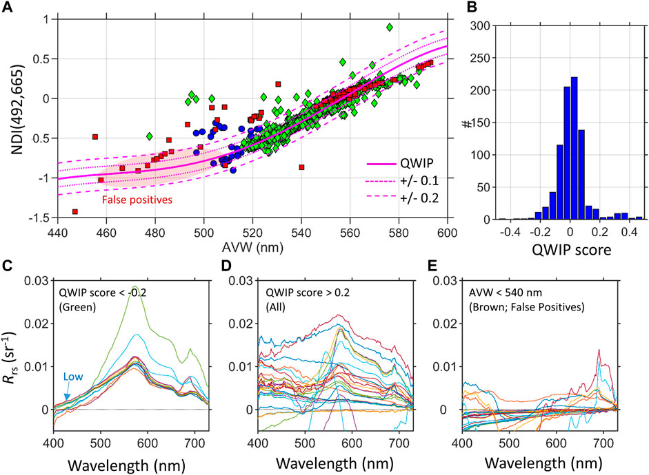
FIGURE 6. (A) The QWIP approach was used for quality control of a raw WISP dataset. Water types include: Blue-green (blue circles), Green (green diamonds) and Brown (red squares) following from Figure 2. The red circle highlights false positive data of brown water type that coincidentally fall within the polynomial limits. (B) The majority of the data had QWIP scores of ±0.2. (C) Remote sensing reflectance (R_rs) of green outliers with slightly negative scores had good spectral shapes but too low in the blue. (D) High QWIP scores were related to the outliers of bad data with unusual spectral shapes. (E) Brown outliers with failing spectral shapes were identified as having lower AVW than expected for the water type (AVW <540 nm).

FIGURE 7

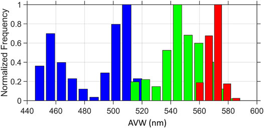
FIGURE 7. Histogram of the distribution of Apparent Visible Wavelength (AVW) from Blue-green (blue), Green (green), and Brown (red) water types showing the overlap and general ranges expected for each water type. Ranges from the CASCK-P training data from Figure 4.

In addition to major outliers, the QWIP score can be useful for diagnosing subtle issues with data quality. For example, R_rs of green outliers with slightly negative scores revealed spectra that were reasonable overall in spectral shape (Figure 6C), but had potentially too low values in the blue range shorter than 440 nm. This is likely due to a high uncertainty in the removal of surface reflected skylight and potentially too high of a ρ value. Hence, the QWIP diagnostic can lead to a more nuanced processing of above water spectra.

We compared the absolute value of the QWIP score with the spectral quality score proposed by Wei et al. (2016) (“Wei score”) on the raw WISP data (Figure 8). As tabulated in Table 1, there was consistency between the two approaches using an absolute value |QWIP| threshold of >0.2 and a Wei score of <0.5, with 737 data points identified as passing in both techniques and 54 data points as failing with both techniques (highlighted as the colored portions of Figure 8). The 12 data points with passing Wei scores and failing QWIP scores had QWIP scores that were just slightly above 0.2 and would pass a screen of QWIP threshold of 0.3, however at the expense of passing spectra in the QWIP score that had failed the Wei score. The Wei approach did correctly fail the “false positive” brown water spectra discussed above. However, there was discrepancy between the two methods in roughly 5% of the dataset. Similar to the PANTHYR data, the Wei score was potentially too low for green data with large red edge reflectance and certain brown water types (Table 1). Such waters can be challenging to assess given the limited band set, particularly in orange and red wavelengths, used in the Wei method. Barnes et al. (2019) also found that several seemingly high quality spectra had very low Wei scores.

FIGURE 8

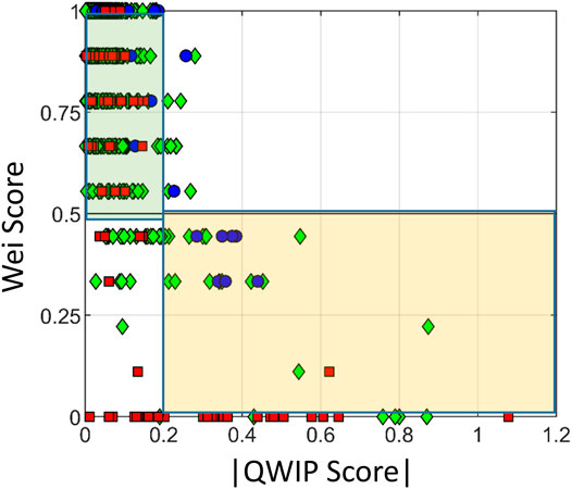
FIGURE 8. Comparisons of the absolute value of the QWIP score with the spectral quality score proposed by Wei et al. (2016) (“Wei score”). A QWIP threshold of >0.2 and a Wei score of <0.5 were considered failing spectra and vice versa. Colored boxes highlight where both approaches pass (green) and fail (yellow) data. Water types include: Blue-green (blue circles), Green (green diamonds) and Brown (red squares) following from Figure 2.

TABLE 1

TABLE 1. Comparison of approaches for WISP Lifewatch data.

3.2 Quality Water Index Polynomial Applied to Satellite Datasets

The QWIP procedure was applied to a hyperspectral HICO image (H2012236112610), covering the complex waters of the Nile Delta, and extending north into the clear waters of the Mediterranean Sea (Figure 9A). Pseudo-true color composites of the HICO imagery can be found in Supplementary Figure S1 (see Supplementary_README.pdf). For this demonstration, a binary exclusion flag was set to distinguish spectra that pass/fail a nominal threshold value, as defined below. Using rigid exclusion criteria, 99.55% of the spectra from the atmospherically-corrected HICO image passed quality control with QWIP score < ± 0.2), while 0.29% fell above the QWIP score threshold, and 0.16% fell below the QWIP score threshold (Figure 9B). The average gradient of integral-normalized R_rs(λ) spectra (as a function of AVW) are plotted for these three scenarios, showcasing instances in which data were above/failed (Figure 9C), between/passed (Figure 9D), and below/failed (Figure 9E) the threshold QWIP score. Most flagged spectra were characterized by continuous negative reflectance either below 500 nm, or above 600 nm, and sometimes both. Note, that anomalous negative data should have been screened out in the SeaDAS processing prior to this analysis.

FIGURE 9

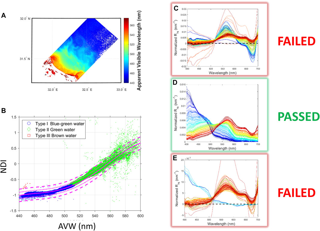
FIGURE 9. (A) Mapped HICO scene on which the QWIP procedure was tested. (B) The AVW is compared to NDI, and (C,E) spectra deviating from the QWIP are nominally deemed to fail quality control criteria, and those (D) within the uncertainty bounds of the polynomial pass. The spectral color scheme relates to the corresponding AVW values, as defined in (A).

Notably, a series of quality flags already exist within the SeaDAS framework to identify pixels that fail various levels of quality control (https://oceancolor.gsfc.nasa.gov/atbd/ocl2flags/). Pixels identified as land (LAND flag), radiance saturation (HILT flag), and clouds or ice (CLDICE flag) are masked during processing (blue in Figure 10), thus no R_rs data were returned for these pixels. The only other standard flags that were indicated over water for this scene were the ATMWARN and MAXAERITER, which indicate a warning in the atmospheric correction procedure, and that the aerosol model reached the maximum amount of iterations, respectively. The ATMWARN flag included all instances of MAXAERITER, and this flag comprises <1% of the ocean pixels (Figure 10) in the HICO scene. The QWIP identified questionable pixels from regions along the edge of the scan line, inland, and even a few offshore patches that were not flagged by ATMWARN (brown regions). In addition, some of the pixels flagged with ATMWARN had spectral shapes with passing QWIP scores (yellow regions).

FIGURE 10

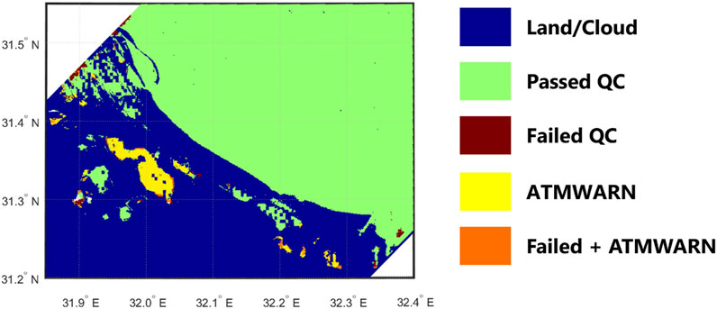
FIGURE 10. A binary quality control (QC) map of a HICO satellite image, illustrating locations in which the NASA processing “l2gen” flags identified pixels with suspect quality (ATMWARN) and pixels identified as either passing (|QWIP|<0.2) or failing (|QWIP|>0.2) QC with the QWIP method. Orange pixels were flagged by both QWIP and l2gen.

A series of additional HICO scenes representing a diverse range of optical water types (H2012237230813, Columbia River outflow, OR, USA; H2014191103614, Danube River Outflow, Romania; H2009344060219, QLD, Australia; see Supplementary Figures S1B–D) were sub-sampled by a range of incremental QWIP score threshold values, to illustrate the connection between QWIP score and spectral shape. Figures 11A−F identify more satellite-derived spectra that failed the nominal quality control criteria, as color coded by discretized QWIP scores. The spectra are often characterized by sharp increases or decreases in the blue range of R_rs(λ) and/or contain negative values. In most cases, as spectral data increasingly deviate from the polynomial relationship between AVW and NDI (492,665), the anomalous spectral features become more prominent.

FIGURE 11

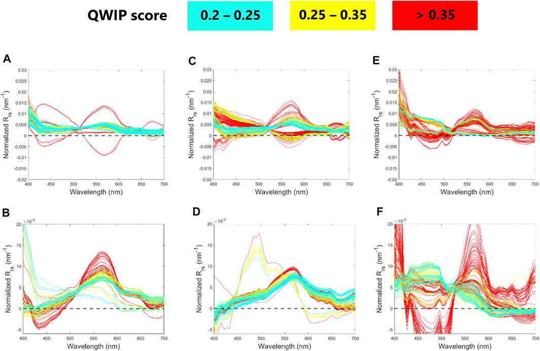
FIGURE 11. HICO spectra that fail quality control criteria by falling above (A,C,E) or below (B,D,F) a nominal QWIP threshold (0.2), for a diverse range of images from the (A,B) Columbia River outflow, USA, (C,D) Danube River outflow, Romania, and (E,F) Queensland, Australia.

3.3 Quality Water Index Polynomial Applied to Multi-Spectral Validation Data

While the QWIP was developed for hyperspectral measurements, the approach can be applied to multi-spectral data using sensor-specific coefficients to derive the hyperspectral-equivalent AVW as per Vandermeulen et al. (2020). Here, we test the algorithm efficacy using multi-spectral validation measurements (in this case, for SNPP-VIIRS) retrieved from NASA’s SeaBASS. In order to use the QWIP as defined in this manuscript, the AVW derived from multi-spectral measurements must first be translated to a hyperspectral-equivalent AVW through the use of sensor-specific polynomial offsets (Vandermeulen et al., 2020). The most recent updates to the coefficients for all satellite sensors processed by OBPG have been developed and published (Vandermeulen, 2022) (also see Matlab scripts in Supplemental Material).

Applying the same procedure as the HICO analysis, 5.2% and 12.1% of the VIIRS satellite data were flagged as falling above/below a QWIP threshold of 0.2, respectively, and 0.2% and 4.2% of in situ data were flagged as falling above/below the QWIP threshold of 0.2. Note, given that SNPP-VIIRS has the fewest number of spectral channels relative to the other validation data streams, it exhibits a higher uncertainty in the calibrated AVW values relative to many other heritage sensors, with a mean absolute error (MAE) of 1.21 nm, and bias of −0.15 nm. Such uncertainty is expected when converting a product derived from five bands into an approximation of its hyperspectral equivalent. To account for this additional uncertainty, we chose here to relax the nominal threshold value to 0.3 for subsequent reporting, as the 0.2 threshold appeared too stringent for practical application.

Using a nominal threshold of 0.3, we found that 2.1% and 8.2% of the VIIRS satellite data were flagged as falling above/below the QWIP threshold, respectively, and 0.0% and 1.0% of in situ data were flagged as falling above/below the QWIP threshold. The flagged spectra were mostly characterized by elevated blue reflectance when the QWIP scores are above the threshold (Figure 12A), and negative/depressed blue reflectance when the QWIP scores are below the threshold (Figure 12B). A scatter plot comparison between in situ (410 nm) and VIIRS (410 nm) R_rs matchups (Figure 12C) shows that the flagged outliers tend to form tightly grouped clusters with independent trends that deviate significantly from the overall linear regression fit. A modest reduction can be seen in the MAE, and bias between the in situ v. satellite matchups for R_rs (412) (Figure 12C), while differences at all other wavelengths were negligible. Notably, the removal of flagged pixels improves the matching of data frequency distributions at R_rs (412) (Figure 12E) relative to the native dataset (Figure 12D).

FIGURE 12

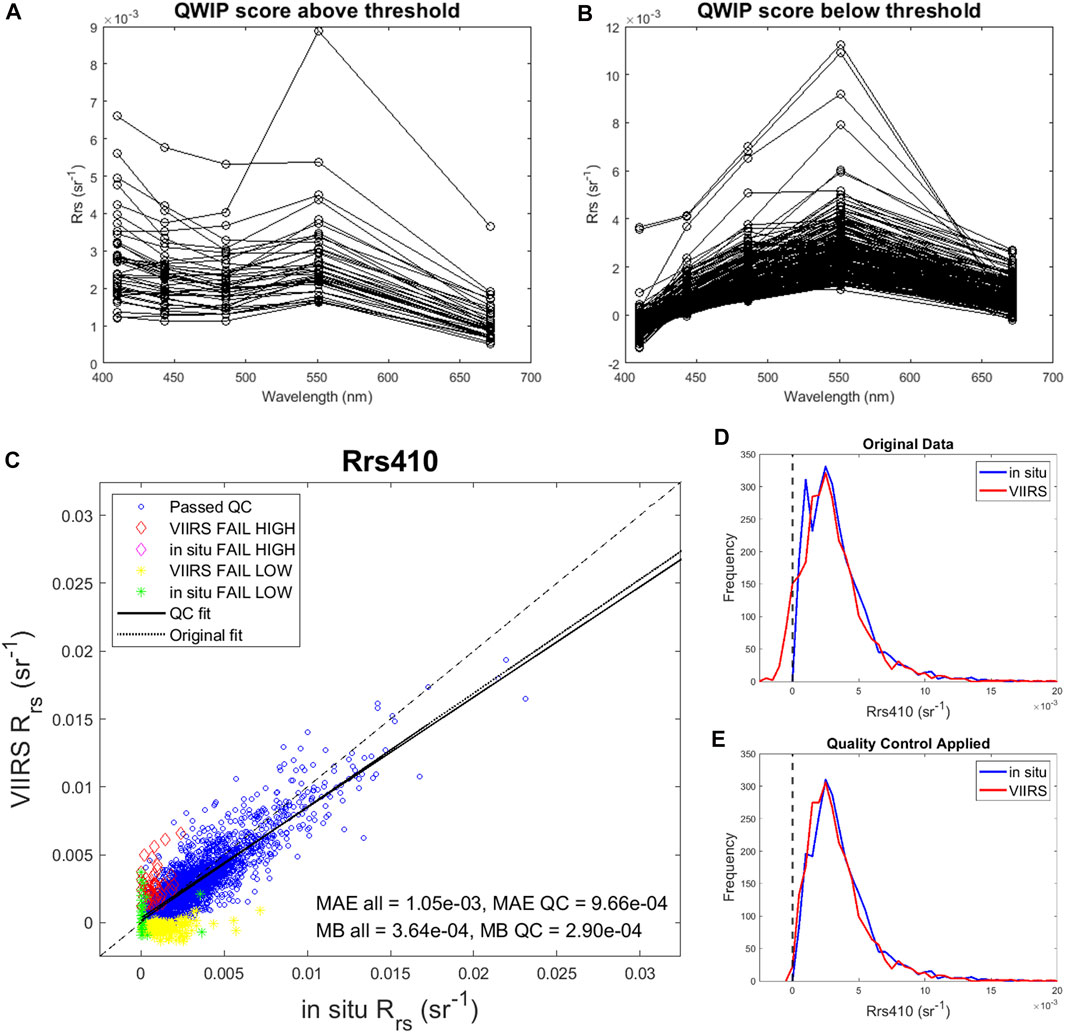
FIGURE 12. Remote sensing reflectance (R_rs) estimated from SNPP-VIIRS that (A) exceeded and (B) fell below a nominal QWIP score of 0.3. (C) Scatter plot of R_rs (410) for in situ obtained from the SeaBASS archive compared to matchup data retrieved from VIIRS imagery. Blue dots represent passing data with QWIP scores less than ±0.3. A modest reduction in mean absolute error and mean bias between in situ and VIIRS measurements was found when only passing values (blue dots) are used. (D,E) The frequency distribution of data improves after the removal of those spectra flagged by the QWIP approach.

4 Discussion and Future Outlook

The QWIP approach provides a simple quantitative tool to evaluate the quality of both field and satellite spectra. The QWIP polynomial based on Apparent Visible Wavelength (AVW) and a red and green band difference index was developed using a broad global training dataset that included blue, blue-green, green, very green with strong fluorescence, and turbid brown waters. A QWIP score represents the spectral deviation from the polynomial with scores less than 0.2 generally considered to be passing. Here, we show how the QWIP can be useful to diagnose major and minor outliers and potentially correctable spectral anomalies like inaccurate removal of surface reflected skylight from above water measurements and provide a quantitative means to screen databases for realistic aquatic spectra both in magnitude and spectral shape. It also has high utility for evaluating different approaches for atmospheric correction of satellite imagery.

The AVW values calculated from field data collected in turbid brown and bright green waters overlapped in magnitude with each other across red wavelengths and were all less than 600 nm. This result is different from the initial work of Vandermeulen et al. (2020) who found values of AVW with increasing chlorophyll up to 617 nm using a synthetic database (Craig et al., 2020). This suggests caution when using synthetic data that has highly sloped backscattering and other features (e.g., inelastic scattering) that may not be representative of real world conditions. The brown and green waters could potentially be better separated with AVW by increasing the spectral range into the near infrared (NIR) out to 800 nm. Tuning the QWIP with AVW calculated from the ultraviolet to NIR wavelengths could provide further discrimination of spectral quality and will be further considered in the future as more datasets become available that cover this larger spectral domain.

Spectra with negative QWIP scores resulted from data that were overcorrected for surface reflected skylight, resulting in lower than expected magnitude in the blue end of the spectrum. Additionally, several optically shallow spectra that were included in the CASCK training dataset were identified as having lower than expected QWIP scores due to the sharp decrease from green to red wavelengths. Future research will evaluate how sensitive this metric is to surface reflected skylight, glint, foam, sensor tilt, and other common issues related to collection of field spectra. Additional analyses will also be conducted to see whether the method can be further adapted to identify a wide variety of optically shallow water spectra including coral reefs, seagrasses, and other benthic features (Garcia et al., 2018; Garcia et al., 2020).

While the QWIP was useful for quality control of a raw field dataset, our research shows that it cannot be the sole quality flag used to process raw datasets. We found obviously bad spectra (i.e., dark spectra with lens covered) that coincidentally had a passing QWIP score. With our training data, these false positives were easily identified by adding an additional screen to limit the range of acceptable AVW for blue, green and brown water types (see Figure 7) or assessing quality using an addition approach like the spectral-matching approach (Wei et al., 2016). While the two approaches yielded very similar results, differences were found between QWIP and Wei scores for certain water types. Specifically, the Wei approach had challenges in assessing the quality of certain green and brown waters compared to QWIP (see Figures 5, 8).

The QWIP approach also proved useful as a quality control metric applied to satellite data. Here, QWIP was successfully used to flag questionable data from atmospherically-corrected ocean color satellite imagery from the hyperspectral HICO, as well as the multi-spectral SNPP-VIIRS. Satellite processing chains do have flags that can identify pixels that fail various levels of quality control; however, those flags can still let through some questionable spectra. Comparisons between VIIRS and in situ match-up data, for example, showed that removal of pixels with high absolute QWIP scores improved the correspondence between the field and satellite data. Additional comparisons between satellite data which is not masked by quality flags would also prove useful. Further improvement could involve development and tuning of sensor-specific polynomial offsets used to extrapolate AVW for multi-channel sensors for more optically complex waters. The technique could also be tested for 3−4 channel broadband “RGB-type” sensors allowing for greater uncertainty.

It is worth emphasizing that the discontinuity in multi-spectral sampling relative to the more continuous hyperspectral measurements creates a bias in the AVW values, and that the QWIP values presented in this manuscript are specifically relevant for 1 nm interval hyperspectral R_rs data. This relationship between multi- and hyperspectral AVW is non-linear, and varies as a function of spectral channels and bandwidth (Vandermeulen et al., 2020; Castagna et al., 2022). In order to use the QWIP on multi-spectral data streams, one of two methods may be employed: 1) convert the multispectral AVW values to a hyperspectral equivalent value, following Vandermeulen (2022), and then utilize the QWIP relationship as presented in this manuscript, or 2) derive an independent multispectral QWIP relationship by subsampling a library of quality-controlled hyper-spectral R_rs to the relevant multispectral wavelengths, and use this information to derive a new QWIP polynomial that would only be used with data of that specific spectral resolution.

Because of its simplicity and highly visual component, we foresee high applicability for the QWIP method across a wide array of applications. Data and scripts we provide in the Supplementary Material would enable users to employ either approach. The quality of various atmospheric correction routines can be quickly assessed by comparing retrieved results to the QWIP. The QWIP can also be used to fine tune approaches used to remove surface reflected skylight and other data processing choices from above water reflectance measurements. The QWIP method provides a simple tool to help evaluate spectral shape and magnitude for a variety of aquatic water-leaving reflectance spectra. Indeed, most researchers are well-equipped to apply the QWIP method to “qwip” their data into shape.

Data Availability Statement

The original contributions presented in the study are included in the article/Supplementary Material, further inquiries can be directed to the corresponding author.

Author Contributions

HD and RV wrote and conceived of this approach and did the primary data analysis and manuscript preparation. BB calculated Wei scores. BB, AC, EK and QV contributed data, wrote methods, and contributed to the final editing of the manuscript. Preliminary PANTHYR data were obtained thanks to platform access, maintenance and installation support of the Institute of Marine Sciences of the Italian National Research Council (CNR-ISMAR) for the AAOT platform, and The Flemish Marine Institute (VLIZ) and POM West-Vlaanderen for the Blue Accelerator platform.

Funding

Funding for this research was provided by BELSPO Stereo III TIMBERS project (SR/00/381) and NASA Ocean Biology and Biogeochemistry (80NSSC20K1518). AC acknowledges funding provided by BELSPO Stereo III PHYTOBEL project (SR/02/213). RV acknowledges funding by the National Aeronautics and Space Administration (NASA) Plankton, Aerosol, Cloud, ocean Ecosystem (PACE) mission.

Conflict of Interest

Author RV was employed by the company Science Systems and Applications Inc.

The remaining authors declare that the research was conducted in the absence of any commercial or financial relationships that could be construed as a potential conflict of interest.

Publisher’s Note

All claims expressed in this article are solely those of the authors and do not necessarily represent those of their affiliated organizations, or those of the publisher, the editors and the reviewers. Any product that may be evaluated in this article, or claim that may be made by its manufacturer, is not guaranteed or endorsed by the publisher.

Acknowledgments

The authors acknowledge all of the individuals who participated in collection of the data used in this paper.

Supplementary Material

The Supplementary Material for this article can be found online at: https://www.frontiersin.org/articles/10.3389/frsen.2022.869611/full#supplementary-material

References

Aurin, D. A. (2022). Hyperspectral in Situ Support for PACE. Available at: https://github.com/nasa/HyperInSPACE.

Google Scholar

Bailey, S. W., Franz, B. A., and Werdell, P. J. (2010). Estimation of Near-Infrared Water-Leaving Reflectance for Satellite Ocean Color Data Processing. Opt. Express 18 (7), 7521–7527. doi:10.1364/oe.18.007521

PubMed Abstract | CrossRef Full Text | Google Scholar

Bailey, S. W., and Werdell, P. J. (2006). A Multi-Sensor Approach for the On-Orbit Validation of Ocean Color Satellite Data Products. Remote Sens. Environ. 102, 12–23. doi:10.1016/j.rse.2006.01.015

CrossRef Full Text | Google Scholar

Balasubramanian, S. V., Pahlevan, N., Smith, B., Binding, C., Schalles, J., Loisel, H., et al. (2020). Robust Algorithm for Estimating Total Suspended Solids (TSS) in Inland and Nearshore Coastal Waters. Remote Sens. Environ. 246, 111768. doi:10.1016/j.rse.2020.111768

CrossRef Full Text | Google Scholar

Barnes, B. B., Cannizzaro, J. P., English, D. C., and Hu, C. (2019). Validation of VIIRS and MODIS Reflectance Data in Coastal and Oceanic Waters: An Assessment of Methods. Remote Sensing Environ. 220, 110–123. doi:10.1016/j.rse.2018.10.034

CrossRef Full Text | Google Scholar

Bulgarelli, B., and Zibordi, G. (2020). Adjacency Radiance Around a Small Island: Implications for System Vicarious Calibrations. Appl. Opt. 59, C63–C69. doi:10.1364/ao.378512

PubMed Abstract | CrossRef Full Text | Google Scholar

Casey, K. A., Rousseaux, C. S., Gregg, W. W., Boss, E., Chase, A. P., Craig, S. E., et al. (2020). A Global Compilation of In Situ Aquatic High Spectral Resolution Inherent and Apparent Optical Property Data for Remote Sensing Applications. Earth Syst. Sci. Data 12, 1123–1139. doi:10.5194/essd-12-1123-2020

CrossRef Full Text | Google Scholar

Castagna, A., Amadei Martínez, L., Bogorad, M., Daveloose, I., Dassevile, R., Dierssen, H. M., et al. (2022). Optical and Biogeochemical Properties of Belgian Inland and Coastal Waters. Earth Syst. Sci. Data. doi:10.1594/PANGAEA.940240

CrossRef Full Text | Google Scholar

Castagna, A., Simis, S., Dierssen, H., Vanhellemont, Q., Sabbe, K., and Vyverman, W. (2020). Extending Landsat 8: Retrieval of an Orange Contra-band for Inland Water Quality Applications. Remote Sensing 12, 637. doi:10.3390/rs12040637

CrossRef Full Text | Google Scholar

Craig, S. E., Lee, Z., and Du, K. (2020). Top of Atmosphere, Hyperspectral Synthetic Dataset for PACE (Phytoplankton, Aerosol, and Ocean Ecosystem) Ocean Color Algorithm Development. National Aeronautics and Space Administration. doi:10.1594/PANGAEA.915747

CrossRef Full Text | Google Scholar

Dierssen, H., Bracher, A., Brando, V., Loisel, H., and Ruddick, K. (2020). Data Needs for Hyperspectral Detection of Algal Diversity across the globe. Oceanography 33, 74–79. doi:10.5670/oceanog.2020.111

CrossRef Full Text | Google Scholar

Dierssen, H. M., Ackleson, S. G., Joyce, K., Hestir, E., Castagna, A., Lavender, S. J., et al. (2021). Living up to the Hype of Hyperspectral Aquatic Remote Sensing: Science, Resources and Outlook. Front. Environ. Sci. 9, 134. doi:10.3389/fenvs.2021.649528

CrossRef Full Text | Google Scholar

Dierssen, H. M., Zimmerman, R. C., Leathers, R. A., Downes, T. V., and Davis, C. O. (2003). Ocean Color Remote Sensing of Seagrass and Bathymetry in the Bahamas Banks by High-Resolution Airborne Imagery. Limnol. Oceanogr. 48, 444–455. doi:10.4319/lo.2003.48.1_part_2.0444

CrossRef Full Text | Google Scholar

Gao, B. C., and Davis, C. O. (1997). Development of a Line-By-Line-Based Atmosphere Removal Algorithm for Airborne and Spaceborne Imaging Spectrometers. Imaging Spectrom. 3118, 132–141.

Google Scholar

Garcia, R. A., Lee, Z., Barnes, B. B., Hu, C., Dierssen, H. M., and Hochberg, E. J. (2020). Benthic Classification and IOP Retrievals in Shallow Water Environments Using MERIS Imagery. Remote Sens. Environ. 249, 112015. doi:10.1016/j.rse.2020.112015

CrossRef Full Text | Google Scholar

Garcia, R., Lee, Z., and Hochberg, E. (2018). Hyperspectral Shallow-Water Remote Sensing with an Enhanced Benthic Classifier. Remote Sens. 10, 147. doi:10.3390/rs10010147

CrossRef Full Text | Google Scholar

Gordon, H. R., and Wang, M. (1994). Retrieval of Water-Leaving Radiance and Aerosol Optical Thickness over the Oceans with SeaWiFS: a Preliminary Algorithm. Appl. Opt. 33 (3), 443–452. doi:10.1364/ao.33.000443

PubMed Abstract | CrossRef Full Text | Google Scholar

Gould, R. W., Arnone, R. A., and Sydor, M. (2001). Absorption, Scattering, and Remote Sensing Reflectance Relationships in Coastal Waters: Testing a New Inversion Algorithm. J. Coastal Res. 17, 328–341.

Google Scholar

Hommersom, A., Kratzer, S., Laanen, M., Ansko, I., Ligi, M., Bresciani, M., et al. (2012). Intercomparison in the Field between the New WISP-3 and Other Radiometers (TriOS Ramses, ASD FieldSpec, and TACCS). J. Appl. Remote Sens. 6, 063615. doi:10.1117/1.jrs.6.063615

CrossRef Full Text | Google Scholar

Ibrahim, A., Franz, B., Ahmad, Z., Healy, R., Knobelspiesse, K., Gao, B.-C., et al. (2018). Atmospheric Correction for Hyperspectral Ocean Color Retrieval with Application to the Hyperspectral Imager for the Coastal Ocean (HICO). Remote Sens. Environ. 204, 60–75. doi:10.1016/j.rse.2017.10.041

CrossRef Full Text | Google Scholar

Knaeps, E., Ruddick, K. G., Doxaran, D., Dogliotti, A. I., Nechad, B., Raymaekers, D., et al. (2015). A SWIR Based Algorithm to Retrieve Total Suspended Matter in Extremely Turbid Waters. Remote Sens. Environ. 168, 66–79. doi:10.1016/j.rse.2015.06.022

CrossRef Full Text | Google Scholar

Lee, Z., Wei, J., Shang, Z., Garcia, R., Dierssen, H. M., Ishizaka, J., et al. (2020). “On-Water Radiometry Measurements: Skylight-Blocked Approach and Data Processing,” in IOCCG Ocean Optics & Biogeochemistry Protocols for Satellite Ocean Colour Sensor Validation.

Google Scholar

Mobley, C. D. (1999). Estimation of the Remote-Sensing Reflectance from Above-Surface Measurements. Appl. Opt. 38, 7442–7455. doi:10.1364/ao.38.007442

PubMed Abstract | CrossRef Full Text | Google Scholar

Mortelmans, J., Deneudt, K., Cattrijsse, A., Beauchard, O., Daveloose, I., Vyverman, W., et al. (2019). Nutrient, Pigment, Suspended Matter and Turbidity Measurements in the Belgian Part of the North Sea. Sci. Data 6, 22–28. doi:10.1038/s41597-019-0032-7

PubMed Abstract | CrossRef Full Text | Google Scholar

Ocean Biology Processing Group (2022). NASA SeaDAS Software Package. Available at: https://seadas.gsfc.nasa.gov.

Google Scholar

O’Reilly, J. E., Maritorena, S., Mitchell, B. G., and Siegel, D. A. (1998). Ocean Color Chlorophyll Algorithms for SeaWiFS. J. Geophys. Res. 103 (24), 937953–938024.

Google Scholar

Qin, P., Simis, S. G. H., and Tilstone, G. H. (2017). Radiometric Validation of Atmospheric Correction for MERIS in the Baltic Sea Based on Continuous Observations from Ships and AERONET-OC. Remote Sens. Environ. 200, 263–280. doi:10.1016/j.rse.2017.08.024

CrossRef Full Text | Google Scholar

Röttgers, R., Doerffer, R., McKee, D., and Schönfeld, W. (2016). The Water Optical Properties Processor (WOPP): Pure Water Spectral Absorption, Scattering, and Real Part of Refractive Index Model. ATBD.

Google Scholar

Ruddick, K. G., De Cauwer, V., Park, Y.-J. J., and Moore, G. (2006). Seaborne Measurements of Near Infrared Water-Leaving Reflectance: The Similarity Spectrum for Turbid Waters. Limnol. Oceanogr. 51, 1167–1179. doi:10.4319/lo.2006.51.2.1167

CrossRef Full Text | Google Scholar

Ruddick, K. G., Voss, K., Boss, E., Castagna, A., Frouin, R., Gilerson, A., et al. (2019). A Review of Protocols for Fiducial Reference Measurements of WaterLeaving Radiance for Validation of Satellite Remote-Sensing Data over Water. Remote Sens. 11, 2198. doi:10.3390/rs11192198

CrossRef Full Text | Google Scholar

Shang, Z., Lee, Z., Wei, J., and Lin, G. (2020). Impact of Ship on Radiometric Measurements in the Field: A Reappraisal via Monte Carlo Simulations. Opt. Express 28, 1439–1455. doi:10.1364/OE.28.001439

PubMed Abstract | CrossRef Full Text | Google Scholar

Tilstone, G., Dall’Olmo, G., Hieronymi, M., Ruddick, K., Beck, M., Ligi, M., et al. (2020). Field Intercomparison of Radiometer Measurements for Ocean Colour Validation. Remote Sens. 12, 1587. doi:10.3390/rs12101587

CrossRef Full Text | Google Scholar

Tzortziou, M., Herman, J. R., Gallegos, C. L., Neale, P. J., Subramaniam, A., Harding, L. W., et al. (2006). Bio-optics of the Chesapeake Bay from Measurements and Radiative Transfer Closure. Estuarine, Coastal Shelf Sci. 68, 348–362. doi:10.1016/j.ecss.2006.02.016

CrossRef Full Text | Google Scholar

Vandermeulen, R. A. (2022). Apparent Visible Wavelength (AVW): NASA Algorithm Theoretical Basis Document. Available at: https://oceancolor.gsfc.nasa.gov/atbd/avw/.

Google Scholar

Vandermeulen, R. A., Mannino, A., Craig, S. E., and Werdell, P. J. (2020). 150 Shades of green: Using the Full Spectrum of Remote Sensing Reflectance to Elucidate Color Shifts in the Ocean. Remote Sens. Environ. 247, 111900. doi:10.1016/j.rse.2020.111900

CrossRef Full Text | Google Scholar

Vanhellemont, Q. (2020). Sensitivity Analysis of the Dark Spectrum Fitting Atmospheric Correction for Metre- and Decametre-Scale Satellite Imagery Using Autonomous Hyperspectral Radiometry. Opt. Express 28, 29948–29965. doi:10.1364/oe.397456

PubMed Abstract | CrossRef Full Text | Google Scholar

Vansteenwegen, D., Ruddick, K., Cattrijsse, A., Vanhellemont, Q., and Beck, M. (2019). The Pan-And-Tilt Hyperspectral Radiometer System (PANTHYR) for Autonomous Satellite Validation Measurements-Prototype Design and Testing. Remote Sens. 11, 1360. doi:10.3390/rs011111360

CrossRef Full Text | Google Scholar

Voss, K. J., Johnson, C. B., Yarbrough, M. A., Gleason, A., Flora, S. J., Feinholz, M. E., et al. (2017). “An Overview of the Marine Optical Buoy (MOBY): Past, Present and Future,” in Proceedings of the D-240 FRM4SOC-PROC1 Proceedings of WKP-1 (PROC-1) Fiducial Reference Measurements for Satellite Ocean Colour (FRM4SOC), Tartu, Estonia, 8–13.

Google Scholar

Wei, J., Lee, Z., and Shang, S. (2016). A System to Measure the Data Quality of Spectral Remote-Sensing Reflectance of Aquatic Environments. J. Geophys. Res. Oceans 121, 8189–8207. doi:10.1002/2016jc012126

CrossRef Full Text | Google Scholar

Zaneveld, J. R. V. (1994). “Optical Closure: from Theory to Measurement,” in Ocean Optics (Oxford University Press). doi:10.1093/oso/9780195068436.003.0007

CrossRef Full Text | Google Scholar

Zhang, X., He, S., Shabani, A., Zhai, P.-W., and Du, K. (2017). Spectral Sea Surface Reflectance of Skylight. Opt. Express 25, A1–A13. doi:10.1364/oe.25.0000a1

PubMed Abstract | CrossRef Full Text | Google Scholar

Zibordi, G., Mélin, F., Berthon, J.-F., Holben, B., Slutsker, I., Giles, D., et al. (2009). AERONET-OC: a Network for the Validation of Ocean Color Primary Products. J. Atmos. Oceanic Tech. 26, 1634–1651. doi:10.1175/2009jtecho654.1

CrossRef Full Text | Google Scholar

Zibordi, G., Voss, K., Johnson, B. C., and Mueller, J. L. (2019). Protocols for Satellite Ocean Color Data Validation: In Situ Optical Radiometry. IOCCG Protocols Document.

Google Scholar