 Asmamaw Gebrehiwot
 Leila Hashemi-Beni
- Geomatics Program, Department of Built Environment, North Carolina A&T State University, Greensboro, NC, United States
Inundation mapping is a critical task for damage assessment, emergency management, and prioritizing relief efforts during a flooding event. Remote sensing has been an effective tool for interpreting and analyzing water bodies and detecting floods over the past decades. In recent years, deep learning algorithms such as convolutional neural networks (CNNs) have demonstrated promising performance for remote sensing image classification for many applications, including inundation mapping. Unlike conventional algorithms, deep learning can learn features automatically from large datasets. This research aims to compare and investigate the performance of two state-of-the-art methods for 3D inundation mapping: a deep learning-based image analysis and a Geomorphic Flood Index (GFI). The first method, deep learning image analysis involves three steps: 1) image classification to delineate flood boundaries, 2) integrate the flood boundaries and topography data to create a three-dimensional (3D) water surface, and 3) compare the 3D water surface with pre-flood topography to estimate floodwater depth. The second method, i.e., GFI, involves three phases: 1) calculate a river basin morphological information, such as river height (hr) and elevation difference (H), 2) calibrate and measure GFI to delineate flood boundaries, and 3) calculate the coefficient parameter (α), and correct the value of hr to estimate inundation depth. The methods were implemented to generate 3D inundation maps over Princeville, North Carolina, United States during hurricane Matthew in 2016. The deep learning method demonstrated better performance with a root mean square error (RMSE) of 0.26 m for water depth. It also achieved about 98% in delineating the flood boundaries using UAV imagery. This approach is efficient in extracting and creating a 3D flood extent map at a different scale to support emergency response and recovery activities during a flood event.
1 Introduction
Flooding is one of the most common and frequently occurring natural hazards that affects lives, property, and the environment around the world (Eccles et al., 2019). Climate change has played a vital role in the current increase in flooding occurrence in last few years. The impacts of flooding such as the loss of lives, properties, infrastructures, and agricultural harvests, cost in the range of millions to billions of dollars per single event in the United States (Huang et al., 2018). For example, Hurricane Harvey in 2017 caused massive flooding in Houston, Texas and the damage associated with it was estimated over $125 billion. Rapid detection and mapping of floods are essential for emergency response, damage assessment, prioritizing relief efforts, and assessing future flood risk.
Remote sensing optical and synthetic aperture radar (SAR) methods have been widely used for flood mapping applications for decades (Shen et al., 2019; Anusha and Bharathi, 2020). The optical sensor can see the world like the human eye and acquire high-resolution data, but it does not work effectively when the site becomes cloudy and dark (Psomiadis et al., 2020). Although SAR is one of the effective sensors to detect flood areas even under cloud cover regardless of time (day/night), it is still challenging to create accurate flood maps using this data due to its spatial resolution and speckle noises (Rahman and Thakur, 2018). Recently, unmanned aerial vehicles (UAVs) have been considered reliable remote sensing sources for acquiring geospatial data for flood mapping applications because of their ability to collect high-resolution imagery with flexibility in the frequency and time of data acquisition (Annis et al., 2020; Coveney et al., 2017). In contrast, their short flight endurance and small-scale coverage remain areas of weakness for their wide-scale implementation in remote sensing.
Several researchers have studied and proposed different remote sensing methods for flood extent mapping (Gao et al., 1996; Long et al., 2014; Feng et al., 2015; Nandi et al., 2017; Gebrehiwot and Hashemi-Beni, 2020a; Gebrehiwot and Hashemi-Beni, 2020b; Gebrehiwot et al., 2021; Hashemi-Beni and Gebrehiwot, 2021). Among these methods, deep learning algorithms such as CNNs have shown promising performance for flood extent mapping. CNN can automatically extract features, learn directly from the input images, and successfully handle large training datasets (Krizhevsky et al., 2012). Recent studies used CNNs to extract two-dimensional (2D) inundation extents automatically and achieved promising results (Gebrehiwot et al., 2019; Peng et al., 2019; Sarker et al., 2019). For example, Gebrehiwot et al. (2019) modified pre-trained fully convolutional neural network (FCNs) models to generate an inundation extent using UAV optical images and achieved more than 95% accuracy on extracting the flood extent compared to 87% accuracy of support vector machine method (SVM). Similarly, Peng et al. (2019) used CNN to generate a flood extent map using pre-Hurricane and post-Hurricane Harvey flood imagery and achieved a precision of 0.9002 and a recall of 0.9302.
In addition to the flood extent, it is essential to monitor inundation levels because they determine the magnitude of floods. Many studies have applied structure from motion (SfM) for flood applications (Meesuk et al., 2012; Meesuk et al., 2015; Hashemi-Beni et al., 2018). The SfM technique is used to reconstruct the objects’ 3D structure from a series of 2D sequential images. Unlike the traditional photogrammetric methods, SfM solves the multi-camera viewing problem, and generates high-density point clouds from high-resolution images (Hashemi-Beni et al., 2018).
In addition to the flood extent mapping methods, many researchers estimated inundation depth using flood models and characteristic analysis (Sanders et al., 2007; Wing et al., 2017). For example, Sanders et al. (2007) investigated the effect of the spatial resolution of digital elevation model (DEM) on the accuracy of floodwater depth estimation using an inundation model. Wing et al. (2017) developed a hydrodynamic-based model for water level estimation. However, the simulation analysis does not always provide accurate results due its dependency to numerous model parameters and hydrological assumptions. This situation is particularly noticeable where limited hydrological data are available. There are also several work proposing to measure floodwater depth based on a 2D water extent map with an associated DEM (Matgen et al., 2007; Schumann et al., 2007; Gebrehiwot et al., 2021). Matgen et al. (2007) used flood extent and lidar data to estimate floodwater depth. The flood extent edges intersected with DEM to calculate the water polygons’ boundary line elevation based on their approach. Similar research was conducted by Schumann et al. (2007), who retrieved the floodwater depth by combining the regression model and TIN generation. Manfreda et al. (2019) developed a DEM-based inundation depth prediction method based on a geomorphic descriptor—GFI. The GFI was first proposed by Samela et al. (2017) to generate flood extent maps in data-poor environments and large-scale analyses based on available information worldwide. This approach was tested in a case study in southern Italy and showed satisfactory performance. This method is particularly suitable for the area where there is data scarcity. However, the method is effective only for a large study area, in which the flow accumulation values of the whole river basin or subbasin are needed to the GFI calculation and floodwater depths analysis. In all of the DEM-based approaches, the accuracy of water depth heavily depends on the quality of flood extent map and DEM accuracy. Since deep learning algorithms such as CNNs have been proven to be an efficient technique for flood extent mapping, integrating deep learning-based water extent maps and DEM is expected to provide high accuracy floodwater depth (Gebrehiwot et al., 2021). Based on that context, this research aims to compare and evaluate the performance of two main state-of-the-art methods for 3D inundation mapping: a deep learning-based image analysis and Geomorphic Flood Index (GFI). To make the methods comparable, the inundation mappings were implemented over the same study area and the same topography information was applied for spatial analyses.
2 Methodology
2.1 Inundation Depth Estimation Using Fully Convolutional Neural Network Image Segmentation and Digital Elevation Model
The research uses the FCN method studied by Gebrehiwot and Hashemi-Beni (2021). Thus, we briefly explain the methodology here, for more details about the method and its implementation please read the reference. The method for estimating a 3D flood map (flood extent and water depth) consists of three main steps: 1) Flood extent map generation, 2) 3D water surface generation, and 3) 3D flood mapping (Figure 1). Each phase of the study is explained in the following sections.
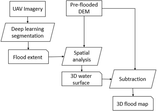
FIGURE 1. Inundation depth estimation using deep learning image classification and DEM.
2.1.1 2D Flood Extent Map Generation
In this stage, the flood extent map is created using a deep learning-based model called FCN-8s. The FCN-8s was proposed by Long et al. (2015) for semantic segmentation application. It is the modified version of the VGG-16 CNN model developed by Simonyan et al. (2014). The network was adjusted so that the convolutional layers replace the fully connected layers of the VGG-16 network. This enables the network to implement pixel-level classification rather than per-image class prediction, as VGG-16 initially used. The study used FCN-8s to delineate the flood boundaries because it applied for flood extent mapping in literature and demonstrated promising results (Gebrehiwot et al., 2019).
The flood dataset including 150 optical UAV images with 4,000 × 40,000 pixels was used to fine-tune and train the FCN-8s. We manually annotated the UAV dataset into a flood, vegetation, and other classes to create training and validation data. During training, the 15-fold cross-validation strategy was used to avoid overfitting the data and improve the performance of the models. For this, we partitioned the data (150 images) randomly into 15 folds. At each run, the union of 14 folds was put together for training the FCN model, and the remaining one-fold was used as a testing or validation set to measure the classification errors. We repeated the above steps 15 times, using a different fold as the testing set each time. Finally, the error from all folds was averaged to estimate the total classification errors. The model is trained using Stochastic Gradient Descent (SGD) algorithm for 10 epochs with a learning rate of 0.001 and a maximum batch size of 2. The FCN-8s is trained by applying data augmentation techniques such as randomly cropping, translation, and random rotation to artificially generate new training data from existing training data (Gebrehiwot et al., 2021). These operations are applied to images in the input space. The study also used the median frequency balancing method to solve the class imbalance issue. Once the FCN-8s network is trained, a flood extent raster is generated for our test area, and it is converted to inundation polygons for further spatial data analysis, integration, and visualization. By spatial overlaying the polygon of permanent waters in Princeville on top of the flood extend results, the floodwater were extracted.
2.1.2 3D Water Surface Creation
This stage will use the hydro flattening concept, assuming that the surfaces of water are flat within each flooded area. The local 3D floodwater surface is created by intersecting the floodwater polygons (plans) with the pre-flood DEM using geospatial analysis. This process assigns an elevation to each polygon vertices. Statistical and spatial analysis will be done to detect and remove noises within each polygon.
2.1.3 3D Flood Mapping
The floodwater depth for each cell in the raster or for each polygon is estimated by subtracting the calculated floodwater surface/elevation from topographic elevation at each grid cell within the flooded area. The elevation difference between the 3D water surface (H) and its corresponding pixel point on the DEM (h) gives the inundation depth (I.D.):
The water depth measurements can be updated based on gauge datum if it needed.
2.2 Inundation Depth Estimation Using Geomorphic Flood Index
2.2.1 Inundation Extent Estimation
This study adopted a hydrogeomorphic method based on the GFI (Manfreda et al., 2019) to generate inundation depth for our study area. Thus, we briefly explained the methodology here, for more details about the method and its implementation please read the reference.
GFI is a descriptor of the basin’s morphology proposed to indicate flood susceptibility in a specific area. This approach provide reliable inundation extent maps in data-scarce regions and large-scale applications (Samela et al., 2017; Manfreda et al., 2019). According to Samela et al. (2017), the GFI at each study point (e.g., green point in Figure 2) is computed as the logarithm of the ratio between river depth (hr) and the elevation difference (H) (see Eq. 1).
Where hr is the river depth, the parameter H represents the difference between the cell’s elevation under exam and the elevation of the above-identified path’s final point. The depth of the river (hr) is estimated as a function of the upslope contributing area using a hydraulic scaling relationship
Where Ar is the contributing area, a is a scale factor, and n is a dimensionless exponent. Based on Eq. 1, locations with GFI values ≥0 are in the flood-prone areas.
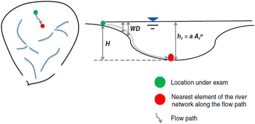
FIGURE 2. A basin cross-section and its parameters to calculate the geomorphic GFI and the inundation depth (Source: Manfreda et al., 2019).
Manfreda et al. (2019) used the GFI approach for floodwater level estimation. The GFI is computed by assuming the coefficient using the threshold calibrated with the linear binary classification. The coefficient is estimated using Eq. 3.
2.2.2 Inundation Depth Estimation
Finally, the water depth (W.D.) within the delineated flood-prone areas estimated by using hr and H as follows (Figure 2):
2.3 Comparison and Evaluation
2.3.1 Flood Extent
The study used a confusion matrix to analyze the accuracy of the FCN-based image classification and the delineation of the flood extent. A confusion matrix provides detailed information on how the classifier is performing. The information include: 1) true positive, i.e., the classification results correctly indicate the positive class as positive; 2) true negative (T.N.), i.e., when the algorithm correctly predicts the negative class as negative (T.P.); 3) false positive (F.P.), i.e. when the classifier incorrectly predicts the negative class as positive; and 4) false negative (F.N.) refers to the number of predictions where the algorithm incorrectly predicts the positive class as negative. In addition to the classification accuracy, the kappa coefficient was used to summarize the information obtained from the confusion matrix. The Kappa coefficient is a metric used to compare an observed accuracy with an expected accuracy or random chance. On the other hand, the performance of the GFI-based flood extent mapping approach is evaluated using the receiver operating characteristic curve (ROC). This curve plots two parameters: True Positive Rate and False Positive Rate at different classification thresholds.
2.3.2 Flood Depth
The study used the RMSE assessment technique to quantify the two methods’ performance in estimating the inundation depth. The RMSE is the square root of the average squared distance between the true and estimated scores and is used as an error metric for predicting quantitative data. The water gauge measurements during the flood events were used as ground truth data to validate and evaluate these inundation depth estimation approaches.
3 Study Area and Data
Two flood-prone areas in North Carolina were selected for the research: Town of Princeville, and the city of Lumberton; because high resolution UAV datasets of the areas during two flooding events were available to the study. The Town of Princeville is located along the Tar River in Edgecombe County in North Carolina (Figure 3). Princeville has gained national attention over the years because of recurring storm flooding. Several flood events have repeatedly affected Princeville for many years since its founding because of its low-lying location. Hurricane Floyd (1999), Hurricane Matthew (2016), and Hurricane Florence (2018) resulted in massive flooding in Princeville and caused enormous destruction and loss of human lives.
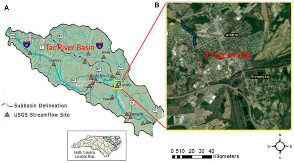
FIGURE 3. Study area: Princeville. (A) The area used to calculate the GFI—Tar River Basin; (B) The study area used for inundation depth calculation for deep learning approach.
Lumberton is a city in Robeson County, North Carolina, United States and is located on the Lumber River in the coastal plains region of North Carolina (Figure 4). The Lumber River has a long history of flooding problems. In the 1960s, the Natural Resources Conservation Service (NRCS) developed a plan to mitigate the flooding issues and allow safer land development for commercial, agricultural, and residential uses. It included constructing a levee system along the Lumber River and operation and maintenance plans to maintain the channels and levee system.
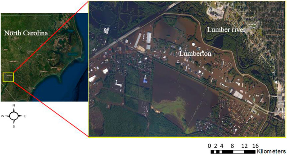
FIGURE 4. The study area used to train the CNN network—Lumberton, NC, and during-event aircraft imagery taken in October 2016.
The data used for the research include:
• UAV Imagery: The UAV high-resolution imagery was captured by the North Carolina Emergency Management (NCEM) during hurricane Matthew in 2016 and Hurricane Florence in 2018 ver the study areas. The size of each image is 4,000 × 4,000, with a resolution of 2.6 cm. The FCN method was employed to segment the UAV imagery into flood and non-flood class and create flood extent map of the study areas.
• LiDAR Data: The pre-flood LiDAR data was used to estimate floodwater depth over the study areas using both method. The LiDAR with two pulses per square meter (pls/m2) with an accuracy of 0.0925 m RMSE was collected by the North Carolina Emergency Management in 2014.
• Flood Map: The Flood hazard map for Hurricane Matthew was employed as an input and for calibration of the GFI method. This map was created by the Natural Conservancy and the Arizona State University center using a random forest algorithm using synthetic aperture radar data (Schaffer-Smith et al., 2019; Schaffer-Smith et al., 2020) (Figure 5).
• USGS Gauge Reading: The USGS water gauge measurements during the flood events were used as ground truth to validate and evaluate the water depth estimations by the methods. The USGS Gauge Stations collect time-series data that describe stream level, streamflow, reservoir and lake levels, surface-water quality, and rainfall. They are used to collect continuous streamflow data year-round. The floodwater depth at the USGS Surface Water Gauge Station, 02083500 Tar River at Tarboro, NC, was collected for evaluation. The Tar River at the Tarboro, NC site is located along with US HWY 64 Business, directly across the Tar River from Princeville (Figure 2B). This site is ideal for measurements of stream levels during a flood event due to its proximity to the study area makes (Hashemi-Beni et al., 2018).
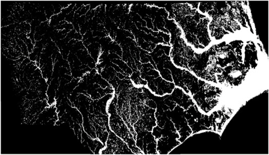
FIGURE 5. Flood extent map of North Carolina during Hurricane Matthew in 2016 Source: (Schaffer-Smith et al., 2020).
4 Results
In this study, the flood extent maps were implemented in MATLAB and Python. The geospatial data integration and spatial analyses were conducted in ArcGIS. The computing unit was configured with 32 GB memory, an Intel(R) Xeon(R) ES-2620 v3 @ 2.40 GHz × 2 processors memory, and a single NVIDIA Quadro M4000 GPU.
4.1 Deep Learning and Digital Elevation Model-Based Inundation Depth Estimation
4.1.1 Inundation Extent Extraction
This section presented the flood extent mapping results obtained using Method 1. Figure 6 shows one sample flood extent result generated using the fine-tuned FCN-8s model. The results shows that the image calcification approach can effectively extract the flooded area from the input image. The overall accuracy calculated by the confusion matrix and kappa index achieved by FCN-8s was about 98% and 0.93, respectively.
FIGURE 6. One sample flood extent map result. (A) Test image; (B) Flood extent map.
4.1.2 Floodwater Depth
Figure 7 shows the flood depth maps generated using the presented approach for the study area. Figure 7B illustrates the inundation map created for the test image (Figure 7A) using FCN-8s. The result shows the FCN-8s accurately extracted the flood extent from the test UAV image. Floodwater depth map results obtained are illustrated in Figure 7C. These maps were created by subtracting water surface raster data and pre-flood DEM using Eq. 1. The highest water depth measured using the proposed method is 1.9—this depth value is recorded in the Tar River area, as shown in Figure 7C (red zone). The site with zero water depth or non-flooded regions is shown in black.
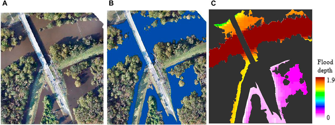
FIGURE 7. Flood depths results; (A) Test image; (B) Flood extent from CNN; (C) Depth result (Unit: meter).
4.2 Geomorphic Flood Index-Based Inundation Depth Estimation Results
For the GFI-based mapping, LiDAR-based DEM and a small portion of the flood hazard map of the basin of interest (The Natural Conservancy and the Arizona State University center) are used as input for mapping and calibration purposes (Figure 5).
GFI approach results the following outputs that are essential to estimate floodwater depth. 1) the water level in each cell of the river network (hr) (Figure 8A); 2) difference in elevation of each DEM cell (basin location) to the nearest river (H) (Figure 8B); 3) derivation of the GFI (Figure 8C); and 4) optimal threshold (τ). The DEM is generated in ArcGIS using LiDAR data. Figure 9 shows the flood depth map generated using GFI in the extent of the deep learning flood map.
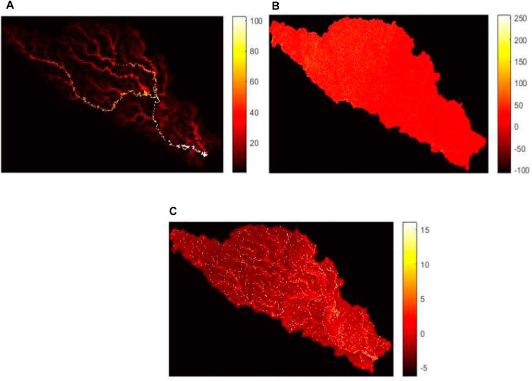
FIGURE 8. Tar River basin morphological features measured form the LiDAR DEM. (A) River depth (hr); (B) Elevation difference (H); (C) Geomorphological flood index (GFI).
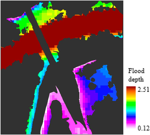
FIGURE 9. Depth results for GFI in the deep learning-based flood extent (Unit: meter).
Then, water level values (hr) in each cell of the river network were used to estimate the floodwater depth (W.D.) in all hydrologically linked cells of the study area estimated using the water level values (hr) in each cell of the river network and the difference in elevation H between the location under examination (H) Eq. 5.
An inundation depth comparison between the two methods is shown in Figure 10. Flood depth maps are compared to determine if the spatial distribution of water depth measurements is correlated. The floodwater depth rasters compared cell-by-cell, and a water depth difference surface was created. A report of statistics calculated from inundation differences maps is also presented in Figure 10B—the performance of the method was evaluated by comparing the I.D.s against the water gauge data. The RMSE measured for the proposed method and GFI using the gauge elevation data is 0.26 and 0.39 m, respectively. Method 1 (image classification) offers better estimation performance than GFI based on the research results.
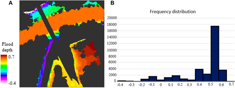
FIGURE 10. Floodwater Depth Comparison. (A) Water depth difference map between the image classification-based method and GFI method; (B) Histograms that shows the distribution of the flood depth difference between the two methods.
The frequency distribution chart shows most of the depth difference recorded between these two methods. The resulting maximum and minimum absolute flood depth differences between GFI and deep learning-based flood map are 0.74 and 0.006 m, respectively. The highest water depth difference values were recorded in the center of the river area. The mean difference value was 0.42 m, with a standard deviation of 0.16 m. The inundation extent map and DEM quality are the two main factors that affect the two approaches’ quality and performance. For various remote sensing applications, including flood mapping, accurate digital DEM is indispensable. Deep learning has been proven to be efficient for segmentation tasks and achieved promising results in extracting flooded areas, reducing the issue of overestimation or underestimating floodwater depths. Overall, using accurate flood extent and DEM can improve the performance of flood depth estimations. In addition, the estimated floodwater depth values give additional information that can use for rescue and damage assessment tasks.
Like the deep learning-based floodwater depth mapping approach, the GFI-based inundation depth mapping approach is highly affected by the quality and accuracy of DEM since the algorithm primarily uses it as input. The pre-flood LiDAR data was used to create DEM in this study for the implementation of the both methods. However, unlike the deep learning method, the GFI approach is unsuitable for estimating floodwater depth for a small area. Because it requires studying an entire hydrographic basin or subbasin to calculate the flow accumulation values coherent with reality (Manfreda et al., 2019). For that purpose, the DEM, slope, flow accumulation, and flow direction of the whole basin or subbasin need to be created as input for any area (small or large) floodwater depth estimation purposes based on the GFI mapping method. Unless this method leads to a wrong result, only if a portion of the basin or subbasin is used.
In contrast, the classification method can effectively estimate floodwater depth for any area of interest (small or large area) because these methods use the flood extent and DEM size equal to the area of interest or the study area. This saves computational time as well as issues related to data shortage. Using an accurate flood extent map is vital to estimate the water level precisely. Inaccurate flood extent extraction can lead to overestimating or underestimating flood depths. Deep learning algorithms such as CNN can automatically create inundation extent from the input images based on training. The FCN-8s trained with Hurricane Matthew (2018) images acquired in Lumberton in this study. The network was tested with Hurricane Florence image obtained in Princeville and achieved more than 98% accuracy.
The integrated method (method 1) seems providing better performance in extracting and creating 3D flood map in comparison with tradition methods such as thresholding and active contour modeling (e.g., Matgen et al., 2007) when the radar signal only gradually increases in the transient shallow water zone between the flooded and the non-flooded areas, and obtaining accurate and timely flood segmentation remains subject to uncertainties. However, the use of SAR data in the studies addressed the segmentation issue in the flooded vegetation areas where the methods based on optical data fail. Regarding the water depth estimation, the integrated method seems being more straightforward approach than traditional hydrodynamic-based models (such as Wing et al., 2017) due to their dependency on numerous model parameters and hydrological assumptions, especially when a limited hydrological data are available for mapping.
5 Conclusion
Flooding is a severe natural hazard that poses a significant threat to human life and property worldwide. Generating an inundation map during extreme flood events is vital for planning and efficiently managing affected areas. This research investigated the performance of deep learning-based image analysis and GFI methods for inundation mapping over the same study areas during the same flooding events. The first method employed a FCN-8s to create a flood extent map using UAV imagery and then, overlaid and integrated the flood extent map with DEM to estimate the floodwater depth. While, the second method only applied the DEM of the study area to calculate the river basin morphological features and estimate water level information to delineate the flood boundaries and measure inundation depth. The performance of the methods were evaluated using the USGS gauge data as ground truth data. The flood water depth RMSE calculated for the deep learning-based image analysis and GFI are 0.26 and 0.39 m, respectively. While the GFI approach is relatively simple to implement, it is unsuitable for estimating floodwater depth for a small area. Because it requires studying an entire hydrographic basin or subbasin to calculate the flow accumulation values coherent with reality. While, the deep learning-based image classification method can be applied for flood mapping at any scale. The results show that the high-resolution image classification offer better estimation for floodwater mapping, minimize the overestimation or underestimation of floods and efficiently create a 3D flood extent map to support emergency response and recovery activities during a flood event.
Data Availability Statement
The data that support the findings of this study are available from the corresponding author upon request.
Author Contributions
LH-B and AG: developed the methodology, implementation, wrote the manuscript.
Funding
This material is based upon work supported by the National Science Foundation (NSF) under Grant No. 1800768: UAV Remote Sensing for Flood Management and NOAA award No. NA21OAR4590358: Rapid Floodwater Extent and Depth Measurements Using Optical UAV and SAR.
Conflict of Interest
The authors declare that the research was conducted in the absence of any commercial or financial relationships that could be construed as a potential conflict of interest.
Publisher’s Note
All claims expressed in this article are solely those of the authors and do not necessarily represent those of their affiliated organizations, or those of the publisher, the editors and the reviewers. Any product that may be evaluated in this article, or claim that may be made by its manufacturer, is not guaranteed or endorsed by the publisher.
References
Annis, A., Nardi, F., Petroselli, A., Apollonio, C., Arcangeletti, E., Tauro, F., et al. (2020). UAV-DEMs for Small-Scale Flood Hazard Mapping. Water 12 (6), 1717.
Anusha, N., and Bharathi, B. (2020). Flood Detection and Flood Mapping Using Multi-Temporal Synthetic Aperture Radar and Optical Data. Egypt. J. Remote. Sens. Space Sci. 23 (2), 207–219.
Coveney, S., and Roberts, K. (2017). Lightweight UAV Digital Elevation Models and Orthoimagery for Environmental Applications: Data Accuracy Evaluation and Potential for River Flood Risk Modelling. Int. J. Remote Sens. 38, 3159–3180. doi:10.1080/01431161.2017.1292074
Eccles, R., Zhang, H., and Hamilton, D. (2019). A Review of the Effects of Climate Change on Riverine Flooding in Subtropical and Tropical Regions. J. Water Clim. Chang. 10 (4), 687–707.
Feng, Q., Liu, J., and Gong, J. (2015). Urban Flood Mapping Based on Unmanned Aerial Vehicle Remote Sensing and Random Forest Classifier—A Case of Yuyao, China. Water 7 (4), 1437–1455. doi:10.3390/w7041437
Gao, B.-c. (1996). NDWI-A Normalized Difference Water Index for Remote Sensing of Vegetation Liquid Water from Space. Remote Sens. Environ. 58 (3), 257–266. doi:10.1016/s0034-4257(96)00067-3
Gebrehiwot, A., and Hashemi-Beni, L. (2020a). A Method to Generate Flood Maps in 3d Using dem and Deep Learning. ISPRS-International Archives of the Photogrammetry, Remote Sensing and Spatial Information Sciences. Washington, DC, USA, 44.
Gebrehiwot, A., and Hashemi-Beni, L. (2020b). Automated Indunation Mapping: Comparison of Methods. In IGARSS 2020-2020 IEEE International Geoscience and Remote Sensing Symposium. Waikoloa, HI, USA: IEEE, 3265–3268.
Gebrehiwot, A. A., and Hashemi-Beni, L. (2021). Three-Dimensional Inundation Mapping Using UAV Image Segmentation and Digital Surface Model. Ijgi 10 (3), 144. doi:10.3390/ijgi10030144
Gebrehiwot, A., Hashemi-Beni, L., Thompson, G., Kordjamshidi, P., and Langan, T. (2019). Deep Convolutional Neural Network for Flood Extent Mapping Using Unmanned Aerial Vehicles Data. Sensors 19 (7), 1486. doi:10.3390/s19071486
Hashemi-Beni, L., and Gebrehiwot, A. A. (2021). Flood Extent Mapping: an Integrated Method Using Deep Learning and Region Growing Using UAV Optical Data. IEEE J. Sel. Top. Appl. Earth Obs. Remote Sens. 14, 2127–2135. doi:10.1109/jstars.2021.3051873
Hashemi-Beni, L., Jones, J., Thompson, G., Johnson, C., and Gebrehiwot, A. (2018). Challenges and Opportunities for UAV-Based Digital. Basel, Switzerland: Environmental Science Sensors.
Huang, X., Wang, C., and Li, Z. (2018). A Near Real-Time Flood-Mapping Approach by Integrating Social Media and Post-event Satellite Imagery. Ann. GIS 24 (2), 113–123. doi:10.1080/19475683.2018.1450787
Krizhevsky, A., Sutskever, I., and Hinton, G. E. (2012). Imagenet Classification With Deep Convolutional Neural Networks. Advances in Neural Information Processing Systems. Lake Tahoe, NV, 25.
Long, J., Shelhamer, E., and Darrell, T. (2015). “Fully Convolutional Networks for Semantic Segmentation,” in Proceedings of the IEEE conference on computer vision and pattern recognition (San Juan, PR, USA: IEEE), 3431–3440. doi:10.1109/cvpr.2015.7298965
Long, S., Fatoyinbo, T. E., and Policelli, F. (2014). Flood Extent Mapping for Namibia Using Change Detection and Thresholding with SAR. Environ. Res. Lett. 9 (3), 035002. doi:10.1088/1748-9326/9/3/035002
Manfreda, S., and Samela, C. (2019). A Digital Elevation Model-Based Method for a Rapid Estimation of Flood Inundation Depth. J. Flood Risk Manag. 12, e12541. doi:10.1111/jfr3.12541
Matgen, P., Schumann, G., Henry, J.-B., Hoffmann, L., and Pfister, L. (2007). Integration of SAR-Derived River Inundation Areas, High-Precision Topographic Data and a River Flow Model toward Near Real-Time Flood Management. Int. J. Appl. Earth Observation Geoinformation 9 (3), 247–263. doi:10.1016/j.jag.2006.03.003
Meesuk, V., Vojinovic, Z., Mynett, A. E., and Abdullah, A. F. (2015). Urban Flood Modelling Combining Top-View LiDAR Data with Ground-View SfM Observations. Adv. Water Resour. 75, 105–117. doi:10.1016/j.advwatres.2014.11.008
Meesuk, V., Vojinovic, Z., and Mynett, A. E. (2012). “Using Multidimensional Views of Photographs for Flood Modeling,” in Proceedings of the 2012 IEEE 6th International Conference on Information and Automation for Sustainability (Beijing, China: IEEE), 19–24.
Nandi, I., Srivastava, P. K., and Shah, K. (2017). Floodplain Mapping through Support Vector Machine and Optical/infrared Images from Landsat 8 OLI/TIRS Sensors: Case Study from Varanasi. Water Resour. Manage 31 (4), 1157–1171. doi:10.1007/s11269-017-1568-y
Peng, B., Liu, X., Meng, Z., and Huang, Q. (2019). “Urban Flood Mapping with Residual Patch Similarity Learning,” in Proceedings of the 3rd ACM SIGSPATIAL International Workshop on A.I. for Geographic Knowledge Discovery (Chicago, IL, USA: IEEE), 40–47.
Psomiadis, E., Diakakis, M., and Soulis, K. X. (2020). Combining SAR and Optical Earth Observation With Hydraulic Simulation for Flood Mapping and Impact Assessment. Remote Sens. 12 (23), 3980.
Rahman, M. R., and Thakur, P. K. (2018). Detecting, Mapping and Analysing of Flood Water Propagation Using Synthetic Aperture Radar (SAR) Satellite Data And GIS: A Case Study From the Kendrapara District of Orissa State of India. Egypt. J. Remote. Sens. Space Sci. 21, S37–S41.
Samela, C., Troy, T. J., and Manfreda, S. (2017). Geomorphic Classifiers for Flood-Prone Areas Delineation for Data-Scarce Environments. Adv. water Resour. 102, 13–28. doi:10.1016/j.advwatres.2017.01.007
Sanders, B. F. (2007). Evaluation of On-Line DEMs for Flood Inundation Modeling. Adv. water Resour. 30 (8), 1831–1843. doi:10.1016/j.advwatres.2007.02.005
Sarker, C., Mejias, L., Maire, F., and Woodley, A. (2019). Flood Mapping with Convolutional Neural Networks Using Spatio-Contextual Pixel Information. Remote Sens. 11 (19), 2331. doi:10.3390/rs11192331
Schaffer-Smith, D., Myint, S., Muenich, R., Tong, D., and DeMeester, J. (2019). Hurricane Flooding and Water Quality Issues. San Francisco, CA, USA: Opportunities for Increased Resilience.
Schumann, G., Hostache, R., Puech, C., Hoffmann, L., Matgen, P., Pappenberger, F., et al. (2007). High-Resolution 3-D Flood Information From Radar Imageryfor Flood Hazard Management. IEEE Trans Geosci Remote Sens. 45 (6), 1715–1725.
Schaffer-Smith, D., Myint, S. W., Muenich, R. L., Tong, D., and DeMeester, J. E. (2020). Repeated Hurricanes Reveal Risks and Opportunities for Social-Ecological Resilience to Flooding and Water Quality Problems. Environ. Sci. Technol. 54 (12), 7194–7204. doi:10.1021/acs.est.9b07815
Shen, X., Wang, D., Mao, K., Anagnostou, E., and Hong, Y. (2019). Inundation Extent Mapping By Synthetic Aperture Radar: A review. Remote Sens. 11 (7), 879.
Simonyan, K., and Zisserman, A. (2014). Very Deep Convolutional Networks for Large-Scale Image Recognition. San Diego, CA, USA: arXiv preprint arXiv:1409.1556.
Keywords: remote sensing, natural disasater, automation, geospatial data modeling, UAV
Citation: Gebrehiwot A and Hashemi-Beni L (2022) 3D Inundation Mapping: A Comparison Between Deep Learning Image Classification and Geomorphic Flood Index Approaches. Front. Remote Sens. 3:868104. doi: 10.3389/frsen.2022.868104
Received: 02 February 2022; Accepted: 17 May 2022;
Published: 20 June 2022.
Edited by:
Bahareh Kalantar, RIKEN, JapanReviewed by:
Vahideh Saeidi, Putra Malaysia University, MalaysiaMila Koeva, University of Twente, Netherlands
Copyright © 2022 Gebrehiwot and Hashemi-Beni. This is an open-access article distributed under the terms of the Creative Commons Attribution License (CC BY). The use, distribution or reproduction in other forums is permitted, provided the original author(s) and the copyright owner(s) are credited and that the original publication in this journal is cited, in accordance with accepted academic practice. No use, distribution or reproduction is permitted which does not comply with these terms.
*Correspondence: Leila Hashemi-Beni, bGhhc2hlbWliZW5pQG5jYXQuZWR1