Empirical Remote Sensing Algorithms to Retrieve SPM and CDOM in Québec Coastal Waters

In most coastal waters, riverine inputs of suspended particulate matter (SPM) and colored dissolved organic matter (CDOM) are the primary optically active constituents. Moderate- and high-resolution satellite optical sensors, such as the Operational Land Imager (OLI) on Landsat-8 and the MultiSpectral Instrument (MSI) on Sentinel-2, offer a synoptic view at high spatial resolution (10–30 m) with weekly revisits allowing the study of coastal dynamics (e.g., river plumes and sediment re-suspension events). Accurate estimations of CDOM and SPM from space require regionally tuned bio-optical algorithms. Using an in situ dataset of CDOM, SPM, and optical properties (both apparent and inherent) from various field campaigns carried out in the coastal waters of the estuary and Gulf of St. Lawrence (EGSL) and eastern James Bay (JB) (N = 347), we developed regional algorithms for OLI and MSI sensors. We found that CDOM absorption at 440 nm [a_g (440)] can be retrieved using the red-to-green band ratio for both EGSL and JB. In contrast, the SPM algorithm required regional adjustments due to significant differences in mass-specific inherent optical properties. Finally, the application of regional algorithms to satellite images from OLI and MSI indicated that the atmospheric correction (AC) algorithm C2RCC gives the most accurate remote-sensing reflectance (R_rs) absolute values. However, the ACOLITE algorithm gives the best results for CDOM estimation (almost null bias; median symmetric accuracy of 45% and R² of 0.78) as it preserved the R_rs spectral shape, while tending to yield positively bias SPM (88%). We conclude that the choice of the algorithm depends on the parameter of interest.

1 Introduction

The ability to operationally monitor coastal water constituents such as colored dissolved organic matter (CDOM) and suspended particulate matter (SPM) is critical to understand the physical, chemical, biological, and geological processes governing the coastal ecosystem. These optically active constituents (OACs) are driving light penetration in the aquatic environment (Kirk, 2011) and major biogeochemical (e.g., van der Molen et al., 2017) and photochemical processes (e.g., Zhang and Xie, 2015). During the last decade, new sensors with a spatial resolution of 10–30 m have improved our ability to observe the spatial variability of ocean color (OC) in coastal areas (e.g., Aurin et al., 2013). As a result, high-resolution OC sensors such as the operational land imager (OLI) onboard Landsat-8 and the MultiSpectral Instrument (MSI) on-board Sentinel-2 platforms have shown their importance as monitoring tools for analyzing the spatial and temporal variability of OACs (e.g., Normandin et al., 2019; Chen et al., 2020). These OC sensors allow studying the spatial and temporal dynamics of these constituents in unprecedented ways (Vanhellemont and Ruddick, 2014; Li et al., 2019; Osadchiev and Sedakov, 2019).

On one hand, locally tuned bio-optical algorithms are needed for accurate retrieval of OACs from operational multispectral sensors due to the great optical diversity found in contrasting coastal zones (e.g., Zheng and DiGiacomo, 2017). On the other hand, prior to the application of bio-optical algorithm, satellite data recorded at the top of atmosphere need to be corrected for atmospheric contribution to compute the bottom of atmosphere radiance/reflectance. As a result, atmospheric correction algorithm development is an active field of research and the number of available models has increased significantly over the last decade (Pahlevan et al., 2021). Therefore, here both bio-optical and atmospheric correction algorithms have been considered for practical application to satellite imagery.

Two types of approaches can be followed to retrieve OACs from the marine reflectance signal. Physics-based models in the form of analytical or semi-analytical algorithms (SAAs) present the advantage of retrieving multiple parameters at the same time and allow to associate error to causes through error analysis and error propagation (Odermatt et al., 2012, and ref. therein). However, SAAs require more spectral information than that offered by sensors with broad spectral bands in the visible such as OLI or MSI. Furthermore, atmospheric correction in coastal region can be quite challenging and provide inaccurate values of remote sensing reflectance (Pahlevan et al., 2021), errors which will be more critical for SAAs than for empirical algorithms based on the band ratio.

Nearshore coastal waters of Québec, specifically the eastern shore of James Bay and the north shore of the estuary and Gulf of St. Lawrence (EGSL), are under the freshwater runoff’s influence from the numerous rivers draining the boreal Canadian shield watersheds. The EGSL is one of the major subarctic estuaries characterized by high phytoplankton production sustained by nutrient-rich upwelling in the lower estuary along the north coast (Le Fouest et al., 2006; Cyr et al., 2015), and by fluvial input loaded with nutrients (Therriault and Lacroix, 1976; Hudon et al., 2017). Freshwater runoff brings CDOM and SPM, which by modifying light attenuation and heating the upper part of the water column (Costoya et al., 2016), can affect photosynthesis and primary production of phytoplankton, macroalgae, and seagrass meadows. James Bay, located south of Hudson Bay, is the land of Cree communities that rely on natural resources to maintain their cultural heritage. However, their fishing and hunting grounds are going through profound changes, notably caused by a decline of the eelgrass (Zostera marina L.) beds, a coastal habitat playing a structuring role in the food web (DFO, 2009). Among factors shaping the growth of eelgrass, photosynthetically available radiation (PAR) is a key limiting parameter (Duarte, 1991). Since PAR attenuation is largely driven by CDOM and SPM, the retrieval of these constituents can significantly improve our ability to develop mitigation strategies by defining areas more prone for eelgrass implantation and to respond to this decline (Murphy et al., 2021). In the EGSL coastal waters, chlorophyll-a varies from 0.2 to 17 mg m⁻³ with a mean (standard deviation) value of 2.6 (±2.3) mg m⁻³ (Araújo and Bélanger, 2022). As shown by Araújo and Bélanger (2022), phytoplankton contribution to the non-water absorption budget is marginal in these waters, making the water color (i.e., the remote sensing reflectance) variability mainly driven by CDOM and SPM. A similar conclusion can be drawn from James Bay waters where coastal waters are even more influenced by CDOM-rich boreal rivers inputs, maintaining the surface salinity below 25 PSU. For these reasons, this study focuses on the retrieval of the main driver of the R_rs, i.e., the CDOM and SPM.

Since 2015, we have conducted several oceanographic campaigns in the lower St. Lawrence estuary (PMZA-RIKI buoy) and in nearshore waters along the north coast of St. Lawrence (Sept-Îles Bay, Manicouagan Peninsula, Forestville) and along the eastern shore of James Bay (Figure 1). These campaigns allowed building a biogeochemical–optical database gathering near-simultaneous remote sensing reflectance (R_rs), inherent optical properties (IOPs), and seawater constituents. The main objective of this study was to investigate empirical relationships linking R_rs with CDOM absorption and SPM. We tested various empirical algorithm formulas published in the literature (e.g., Matthews, 2011; Dorji and Fearns, 2016; Houskeeper et al., 2021) with known potential and drawbacks for their application to modern multispectral sensors. The specific objectives were: 1) to develop empirical algorithms for Landsat-8 and Sentinel-2 satellite missions for the Québec coastal waters; 2) to examine the similarity and/or differences between the coastal zones in terms of optical properties and their implications for satellite remote sensing of CDOM and SPM; and 3) to validate the satellite retrievals using OLI and MSI through a matchup analysis. The validation is made with a comparison of six atmospheric correction algorithms.

FIGURE 1

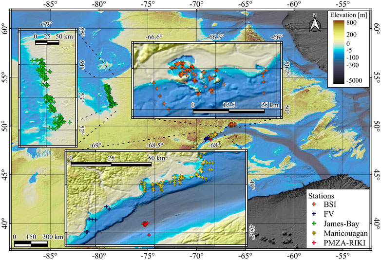
FIGURE 1. Localization map of the datasets, colors correspond to the different areas in which the data were acquired.

We first present the sampling strategy and materials and methods used to build the optical database. Next, we focus on the empirical algorithm development based on in situ data, which highlights similarities and differences among coastal regions. The third section will present the validation of satellite retrievals, based on a matchup analysis of the OLI and MSI sensors with the in situ database. Finally, the main findings in terms of satellite retrievals of SPM and CDOM after the application of atmospheric correction (AC) are discussed.

2 Materials and Methods

2.1 Study Area and Sampling

Acquisition of in situ data has been made within the scope of four different research projects from 2015 to 2019. More detailed information about the projects in the EGSL can be found in Bélanger et al. (2017) and Araújo and Bélanger (2022). Briefly, the lower St. Lawrence estuary was sampled within the framework of the Programme de monitorage de la zone Atlantique (Atlantic Zone Monitoring Program) PMZA (AZMP), initiated and maintained by Fisheries and Oceans Canada (DFO). The station PMZA–RIKI (Figure 1, red symbol), offshore Rimouski, has been visited on 19 occasions in 2015 as detailed in Bélanger et al. (2017). In-water radiometric measurements were performed for the determination of Apparent Optical Properties (AOPs). Concurrently, an optical package was deployed for the determination of bulk IOPs, including particulate backscattering coefficient (b_bp). Along with the IOPs and AOPs, a suite of biogeochemical and optical variables were obtained from discrete water samples, including SPM, spectral CDOM, and particulate absorption coefficients (a_g and a_p).

Within the scope of the Canadian Healthy Oceans Network (CHONe2), 11 field campaigns were conducted in the Bay of Sept-Îles (BSI) area from August 2016 to June 2019 (Figure 1; orange symbols) (for details, see Table 2 in Araújo and Bélanger, 2022). The sampling stations include nearshore coastal waters and optically shallow waters (∼120 stations). In September 2017, with the collaboration of the DFO and the Canadian Hydrographic Service (CHS), fieldwork in support of airborne hyperspectral imagery acquisition was carried along the northern shore of the EGSL. This campaign includes 7 stations in the Forestville (FV) area, sampled on 11 September, where the above-mentioned optical and biogeochemical dataset were collected (Figure 1; black symbols). Finally, in August 2019, a field campaign was organized in the frame of the WaterSat Imaging Spectrometer Experiment in nearshore coastal waters of the Manicouagan Peninsula (Figure 1; yellow symbols), during which more than 50 stations were visited to record optical and biogeochemical data. For all these field campaigns, the protocols detailed in (Bélanger et al., 2017) were followed to compute the desired AOPs, in situ IOPs, and biogeochemical and optical measurements (see below).

The nearshore coastal waters of eastern James Bay were sampled within the framework of a multidisciplinary project in collaboration with the Cree nation to better understand the evolution of eelgrass meadows observed over the last 3 decades (Figure 1; green symbols). The sampling was performed in August–September 2018 and July–August 2019 with the freighter canoes piloted by members of the Cree communities. Due to logistic constraints, different protocols were adopted for in-water AOPs and IOPs (see following subsections).

A total number of 186, 188, and 132 concomitant measurements of R_rs with SPM concentration (C_SPM), a_g, and b_bp, respectively, were available in the EGSL. In James Bay, 161, 155, and 144 concomitant measurements of R_rs with C_SPM, a_g, and b_bp, respectively, were available.

2.2 Derivation of R_rs

Derivation of R_rs (Eq. (1)) follows the NASA protocol (Mueller et al., 2003). Underwater measurement of upwelling radiance L_u (z) and above water measurement of downwelling irradiance E_d (0⁺) were made with different instruments and methods in the EGSL and JB. In the EGSL, vertical profiles of upwelling radiance, L_u (λ, z), where λ is spectral wavelength in nm and z is depth of observation, were measured at 19 wavelengths with different Compact-Optical Profiling System instruments (Morrow et al., 2010). Seventeen common wavelengths were available for the various C-OPS instruments used in the EGSL: 320, 340, 380, 412, 443, 465, 490, 510, 532, 550 (or 560), 589, 625, 665, 683, 694, 710, and 780 nm. In James Bay, underwater hyperspectral upwelling radiance [L_u (z)] below the sea surface (∼5–15 cm depth) was measured using two Satlantic HyperOCR radiometers (HOCR) held away from the boat with a pole and submerged at two different depths, allowing an estimation of the spectral diffuse attenuation coefficient for the upwelling radiance $(K_{L_{\text{u}}})$. The acquisition spectrum of the HOCR spans from 380 to 800 nm by a 3 nm step. In all cases, the incident E_d (0⁺) was measured above water using a radiometer attached to the boat above the structure to avoid shadow. All radiometers were calibrated by the manufacturer less than a year before or after the deployment. In-water radiometry data was processed using the open-source R-packages “Cops” and “HyperocR” available on GitHub (https://github.com/belasi01/). A detailed discussion about the C-OPS instrument and the processing protocols can be found in previous studies (Mueller et al., 2003; Morrow et al., 2010; Antoine et al., 2013; Hooker et al., 2013; Bélanger et al., 2017). Briefly, the processing includes the extrapolation of L_u (z) to the sea surface using the estimated value for $K_{L_{\text{u}}}$ and its transmission across the air-water interface to provide L_w (0⁺), which is used to estimate the remote sensing reflectance:

$R_{\text{rs}}=\frac{L_{\text{w}}\left(0^{+}\right)}{E_{\text{d}}\left(0^{+}\right)}.(1)$

Instrument’s self-shadow correction was applied to C-OPS data following the procedure described by Gordon and Ding (1992) and Zibordi and Ferrari (1995), but considered negligible for HOCR (radius of 3 cm). Radiometric variables were measured at different spectrum limits and were interpolated to obtain values at the same wavelengths through the database. The spectral interpolation (generally a few nanometers) error is assumed to be negligible. We also computed a sensor-equivalent R_rs from our in-water spectral radiometric measurements for OLI and MSI sensor bands through the Relative Spectral Response (RSR) function to develop empirical algorithms specifically for those sensors and to conduct the matchup analysis. Due to the difference in spectral sampling in the near-infrared between C-OPS and HOCR, we could expect some discrepancy between the EGSL and JB dataset for the R_rs (740) channel of MSI.

2.3 Particulate Backscattering

The volume scattering function (VSF) in the backward direction of light propagation was measured with four different backscattering meters: a Hydroscat-6 from HOBI Labs, and ECO-VSF, BB3, and BB9 from Wetlabs. The Hydroscat-6 was used for the sampling of PMZA-RIKI, FV, BSI, and Manicouagan peninsula. Hydroscat-6 measures the VSF at 141° at six waves bands centered at 394, 420, 470, 532, 620, and 700 nm. The BB9 was used at a few stations during WISE-Man (wavebands: 412, 440, 488, 510, 532, 595, 650, 676, and 715 nm). In James Bay, the ECO-VSF (wavebands: 470 and 532 nm) and BB3 (wavebands: 470, 532, and 715 nm) were used in 2018 and 2019, respectively. The Hydroscat-6, mounted on an optical package, which also included a CTD (conductivity-temperature-depth; SBE19 from Seabird scientific) and an a-sphere (HOBI Labs) to measure the total non-water absorption coefficient for vertical profiles of IOPs along the water column. After depth discretization, the data point closest to the surface is selected. Similarly, the BB9 was deployed together with a CTD and an AC-s meter. In James Bay, the BB3 and the ECO-VSF were held by hand in surface water for ∼2 min, and the average value was retained. The raw VSF data, measured at given scattering angle (i.e., ∼ 124° for the ECO-BB and ∼141° for Hydroscat-6; Doxaran et al., 2016), were converted in physical unit (m⁻¹ sr⁻¹) using the manufacturer calibration coefficients with updated dark offsets taken on the field. The conversion of the VSF into a backscattering coefficient (b_b) was performed following the procedure described in Doxaran et al. (2016) for ECO-BB and Hydroscat-6 and in Boss et al. (2004) for the ECO-VSF. The corrections included the loss of signal due to the absorption of the backscattered photons along the optical path length, which was estimated using absorption coefficients for the a-sphere or the AC-s when available, or from the absorption coefficients of CDOM and particles determined on discrete samples (Bélanger et al., 2017; Araújo and Bélanger, 2022). On a few occasions in James Bay, the ECO-BB meters saturated in very turbid waters and the data was flagged.

2.4 Discrete Water Sample Measurements

Water samples were taken near the surface with a bucket or a Niskin bottle, stored away from light and heat in coolers. They were processed in the laboratory as soon (less than 8 h after collection) as the boat returned to harbor. To trace CDOM concentration, spectral absorption coefficients, a_g, were made according to the IOCCG (2018) protocol. Briefly, two filtration steps allow removing all particulate matter, a prefiltration on Whatman GF/F (0.7 µm nominal particle size retained) followed by filtration on Nucleopore 0.2 µm nominal pore size. The absorbance was obtained using a Perkin Elmer double-beam Lambda-850 with quartz cells on 10 cm, 5 cm, or 1 cm path lengths (depending on the concentration) against nano pure water as the reference. The raw data were converted to absorption, and corrected for null offset in the NIR with open source R packages, RspectroAbs, and CDOM available on GitHub (https://github.com/belasi01/RspectroAbs; https://github.com/PMassicotte/cdom).

C_SPM were determined following the recommendations of Neukermans et al. (2012b). Whatman GF/F filters of 47 mm diameter, which effectively retained particles larger than about ∼0.7 µm, were rinsed with distilled water, dried and weighted with a high precision microbalance. Each water sample (volumes depended on turbidity evaluated using the Secchi depth) was filtered in triplicates to assess variation of the measured C_SPM. Additionally, the loss on ignition technique was used by placing the filters at 450°C for 4 hours to determine the fraction of inorganic matter (PIM) and organic matter (POM) in the total SPM pool.

2.5 Algorithm Development and Performance Metrics

For the remote sensing algorithm development, the dataset is divided into training and testing datasets at approximately 70 and 30%, respectively. All regressions were made using the training set, while the performance metrics were calculated on the testing set. Following the recommendations of Seegers et al. (2018), we used three metrics to measure individual algorithms performance and compare them. As outliers may be present (e.g., unflagged optically shallow waters) in our dataset, we choose to compare the accuracy metrics of the relative error (RE) computed with the mean (Mean RE) and the median (Med RE). The former is sensitive to outliers, while the latter is not. Bias is measured with the median of the error, minimizing the impact of the outliers and giving the algorithm systematic error from the bulk of the observation. To assess the relative efficiency of atmospheric correction algorithms, we have used a pairwise comparison metric. Briefly, this method allows the selection of the algorithm with the least residuals (ŷ−y) for each observation. Then, the number of times an algorithm is chosen instead of its competitors is used to compute the percent wins.

To facilitate comparison with the latest literature on atmospheric correction algorithms performance published in Pahlevan et al. (2021), we chose to report the median symmetric accuracy (MdSA, Eq. 3) and the symmetric signed percentage bias (SSPB, Eq. (2)). For a detailed description of those metrics and their proprieties, the reader is referred to Morley et al. (2018).

$\text{SSPB}=100\text{sign}\left(z\right)\left(10^{|z|}-1\right)\left[\%\right]\text{\hspace{0.17em}where\hspace{0.17em}}z=\text{Median}\left({\text{log}}_{10}\left({\widehat{R}}_{\text{rs}}\left({\mathrm{\lambda }}_{\text{i}}\right)/R_{\text{rs}}\left({\mathrm{\lambda }}_{\text{i}}\right)\right)\right),(2)$

$\text{MdSA}=100\left(10^y-1\right)\left[\%\right]\text{\hspace{0.17em}where\hspace{0.17em}}y=\text{Median}|{\text{log}}_{10}\left({\widehat{R}}_{\mathrm{r}\mathrm{s}}\left({\mathrm{\lambda }}_{\text{i}}\right)/R_{\text{rs}}\left({\mathrm{\lambda }}_{\text{i}}\right)\right)|,(3)$

where ${\widehat{R}}_{\text{rs}}({\lambda }_{\text{i}})$ is the retrieved remote sensing reflectance by the satellite at a specific wavelength and R_rs is the measured remote sensing reflectance. They can be replaced by C_SPM or a_g (λ_i) to compute their specific MdSA and SSPB.

2.6 Match-Up Exercise and Atmospheric Correction Comparison

The regional algorithms were applied to satellite imagery from Sentinel-2 and Landsat-8 for which coincident in situ data were available. In total, 72 in situ matchups where found at an interval of ±3 h, 62 with MSI, and 10 with OLI. The matchup data points constitute the testing datasets. L1C images of Landsat-8 OLI and Sentinel-2 MSI A and B, corresponding to a day of an in situ acquisition, were downloaded. We applied six atmospheric correction algorithms:

1 Case 2 Regional Coast Color (C2RCC) (Brockmann et al., 2016);

2 Case 2 extreme (C2X) (Brockmann et al., 2016);

3 Atmospheric Correction for OLI lite (ACOLITE) using the dark spectrum fitting algorithm option (Vanhellemont and Ruddick, 2018; Vanhellemont, 2019a,b, 2020; Vanhellemont and Ruddick, 2021);

4 Sea-viewing Wide Field-of-view Sensor Data Analysis System (SeaDAS) (Franz et al., 2015; Pahlevan et al., 2017);

5 Spectral Shape Parameter (SSP) implemented in SeaDAS (Singh et al., 2019);

6 Image Correction for atmospheric effect (iCOR) (Keukelaere et al., 2018).

C2RCC and C2X are artificial neural network-based models trained with a synthetic dataset generated from radiative transfer simulations of various oceanic and atmospheric conditions. The difference between C2RCC and C2X is that the latter is trained with more extreme cases of optically complex waters, like CDOM-rich and very turbid waters. The others algorithms belong to the tow-steps family. First, they remove the effect of Rayleigh scattering and gaseous absorption using pre-computed look-up-tables (LUTs). The second step estimates the aerosol contribution to the Rayleigh-corrected reflectance. The algorithms are based on different assumptions. For example, SeaDAS is based on the black pixel assumption in the near infrared (NIR) and use it as a baseline to extrapolate the contribution of aerosol in the rest of the spectrum (Gordon and Wang, 1994). The black pixel assumption in the NIR does not hold true in turbid waters where significant amount of light in the NIR (Ruddick et al., 2000). The SSP algorithm is an addendum to the SeaDAS processor to estimate aerosol contribution with the assumption of a non-zero water-leaving radiance in the UV and in the NIR. The ACOLITE and iCOR models are image-based algorithms originally designed to retrieve aerosol optical thickness (AOT) over land surfaces, but with additional correction for water (sky glint corrections). They were adapted to retrieve AOT from the darkest pixels found in a sub-scene (e.g. dense dark vegetation or clear waters). These algorithms have been chosen because they are specifically designed to perform atmospheric correction in coastal waters and are freely available online. After image processing, 44 matchups out of 72 were valid, from which 36 were in the BSI and 8 in JB. Following the methodology described in Pahlevan et al. (2021), the median pixel value was extracted from a 150 m by 150 m box surrounding the measurement location.

3 Results

3.1 Exploratory Data Analysis

The histograms of SPM and CDOM (Figure 2) show different distributions in the EGSL and JB. C_SPM follows a log-normal distribution in the EGSL, while in JB, the distribution is negatively skewed, and presents a higher range of concentrations. CDOM concentration, as expressed by the a_g (440) proxy, exhibits a bimodal distribution in both regions, which is more obvious in JB. In addition, a higher CDOM background is present in JB with most values ranging between 1 and 3 m⁻¹, but with frequent values $>3{\mathrm{m}}^{-\mathrm{1}}$. In addition, the spectral slope (S) of the CDOM spectra was slightly steeper in JB compared to EGSL. The S calculated for 350–500 nm spectral range of 0.0175 ± 0.0006 and 0.0167 ± 0.0010 nm⁻¹ for JB and EGSL, respectively.

FIGURE 2

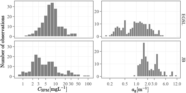
FIGURE 2. Histograms showing the distribution of C_SPM and a_g (400) in the EGSL and JB.

Figure 3 shows the relationships between R_rs at four wavelengths with C_SPM, b_bp (532) and a_g (440). The relationship between C_SPM and R_rs is almost null at 440 nm and becomes positively stronger at longer wavelengths. At 560 nm, the relation is strongly dependent on CDOM concentration (color of the dots), meaning that for a given remote sensing reflectance, high C_SPM are associated with higher CDOM concentration. In JB, for example, for an R_rs value of 0.004 sr⁻¹, we found a_g (440) and C_SPM values of 1 m⁻¹ and 2 mgL⁻¹, respectively, then 4 m⁻¹ and 11 mgL⁻¹, and finally 8 m⁻¹ and 42 mgL⁻¹. If we plot a linear relationship between C_SPM and R_rs, in JB alone, we find that as CDOM increases, the intercept of the relationship also increases. In the same way, but with different relationships, the EGSL R_rs versus C_SPM and CDOM seem to be linked. As CDOM concentration increases, R_rs (560) decreases even if C_SPM increases. These results indicate a significant role of CDOM for the green reflectance in both coastal zones.

FIGURE 3

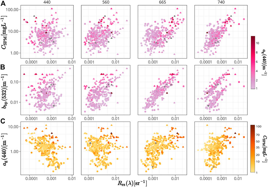
FIGURE 3. Relation between R_rs at 440, 560, 665, and 740 nm, and (A) C_SPM, (B) b_bp (532), and (C) a_g (440). Plot (A) and (B) colors correspond to a_g (440) to assess covariance patterns. Similarly, plot (C) colors correspond to C_SPM in square root space. Triangles and circles represent data from JB and the EGSL, respectively. Grey color represent missing values.

C_SPM versus R_rs in the red (665 nm) also revealed regional differences between the EGSL and JB. For a C_SPM of 10 mgL⁻¹, R_rs is ten times higher in JB than in EGSL. It also shows that the strength of the correlation is weaker in the EGSL comparatively to JB, with a Spearman correlation coefficient of 0.33 and 0.79, respectively. The strongest relationship between R_rs with C_SPM in the two regions is found in the near infrared (740 nm), a spectral region where CDOM is known to have negligible influence on R_rs. The linear relationship for both regions converge (similar slope and intercepts) and higher coefficients of correlation of 0.37 and 0.80 for EGSL and JB, respectively, are reached. Interestingly, at 800 nm (not shown), the two distinct groups, visible at 665 nm, appear again, but the Spearman correlation coefficient (r) reaches its highest values of 0.46 and 0.81 for the EGSL and JB, respectively.

Knowing that remote sensing reflectance is proportional to particulate backscattering coefficient, an inherent optical property (IOP), we further examine the relationship between R_rs and b_bp measured in the green at 532 nm. Figure 3B indicates that the particles sampled in the EGSL and JB likely have distinct specific optical properties. First, the strongest relationship between b_bp (532) and R_rs was found in the red band (665 nm) with no difference between JB and the EGSL. Second, a regional distinction is found at 740 nm, where a linear relationship would yield different intercept, but similar slope. Lower b_bp (532) values for identical R_rs (740) is found in the EGSL compared to JB, indicating that the spectral slope of b_bp or particulate absorption coefficients (a_p) in the NIR are not the same in both regions. Hence, it confirms the regional differences previously observed from the C_SPM versus R_rs relationships. The relationships between the absorption of CDOM at 440 nm and R_rs at the same four wavelengths are shown in Figure 3C. Absorption spectrum of CDOM shows an exponential decay toward longer wavelengths. As expected, knowing the inverse relationship between R_rs and absorption, stronger negative correlation is found at 440 nm than at 560 nm. However and as previously stated for C_SPM, the trend of the a_g (440) relation with R_rs is impacted by C_SPM through the b_bp, but this time with higher R_rs value for high CDOM and C_SPM events. As we move toward longer wavelengths, at 665 and 740 nm, the relation of a_g (440) and R_rs become positive, meaning a potential co-variation between CDOM and particle backscattering and/or SPM, or a direct contribution of CDOM to particle backscattering. However, even at 740 nm, CDOM is suspected to have a significant absorption power. Indeed, the C_SPM concentration follows a diagonal gradient from the top left to bottom right; it shows the interaction of a_g and SPM on R_rs (740), with lower R_rs associated with high a_g (440) and low C_SPM values. Contrary to the C_SPM versus R_rs relationship, we found no difference in a_g (440) with R_rs relation between the EGSL and JB. This indicates that a single algorithm can be fitted to retrieve a_g (440) from marine reflectance.

The mass-specific particulate backscattering ($b_{\text{bp}}^{\ast \mathrm{S}\mathrm{P}\mathrm{M}}=b_{\text{bp}}/C_{\text{SPM}}$, in m²g⁻¹), is a physical quantity used to study the backscattering efficiency of SPM (e.g., (Neukermans et al., 2012a). On average, $b_{\text{bp}}^{\ast \mathrm{S}\mathrm{P}\mathrm{M}}(532)$ of 0.0140 and 0.0021 m² g⁻¹ was found in JB and the EGSL, respectively, indicating that particles are six times more efficient at scattering light in JB compared to those in EGSL. More specifically, we found a negative relationship between C_SPM and $b_{\text{bp}}^{\ast \mathrm{S}\mathrm{P}\mathrm{M}}(532)$ (Figure 4A) in the EGSL, but not in JB. As a result, in the EGSL, as C_SPM increase b_bp will stay approximately the same and $b_{\text{bp}}^{\ast \mathrm{S}\mathrm{P}\mathrm{M}}$ decrease. In JB, in contrast, the slightly positive relationship of C_SPM versus $b_{\text{bp}}^{\ast \mathrm{S}\mathrm{P}\mathrm{M}}$, yields a stronger positive correlation between C_SPM and b_bp and indicates an additive effect of C_SPM on b_bp.

FIGURE 4

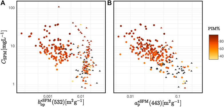
FIGURE 4. (A) Mass-specific particulate backscattering at 532 nm versus C_SPM, (B) mass-specific absorption at 443 nm versus C_SPM. Color corresponds to PIM fraction of total C_SPM, in percent. Black points correspond to the absence of PIM data.

Regarding the mass specific particulate absorption at 443 nm, a difference of magnitude is found between the JB and the EGSL, with an average of 0.083 m²g⁻¹ and 0.033 m²g⁻¹, respectively. A similar negative relationship was found between $a_{\text{p}}^{\ast \mathrm{S}\mathrm{P}\mathrm{M}}$ and C_SPM in both regions (Figure 4B).

3.2 Empirical Algorithms Development

3.2.1 Colored Dissolved Organic Matter Retrieval

Normalization functions such as band ratio algorithms show great potential to assess a_g (λ) accurately. In lower wavelengths, a_g is the main OAC responsible for the total absorption in nearshore zones of the EGSL (Araújo and Bélanger, 2022) and in JB. Thus, its variability can be directly related to the ratio of a wavelength sensitive to its absorption spectrum to a wavelength insensitive to it (Gitelson et al., 1993). Furthermore, band ratio algorithms are less sensitive to atmospheric correction errors (see section 3.3.2), as the ratio will diminish a part of the error. Building up on published studies and the exploratory analysis above, we tested relationships between a_g and R_rs ratio using non-linear algorithms with the non-linear least square (nls, Gauss-Newton algorithm) function of R. Only the best relationships are shown in Figure 5 and Table 1.

FIGURE 5

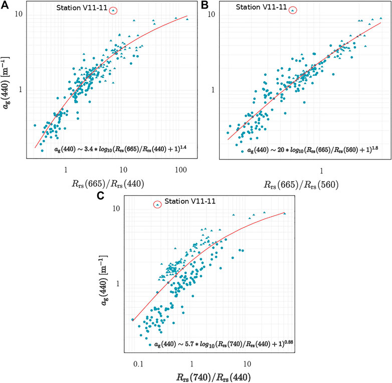
FIGURE 5. Nonlinear empirical algorithms for a_g (440) on log-log space by (A) band ratio R_rs (665)/R_rs (440), (B) band ratio R_rs (665)/R_rs (560), and (C) band ratio R_rs (740)/R_rs (440). Continuous line corresponds to fitted values. Circles and triangles correspond to the data acquired in the EGSL and in JB respectively. Station V11-11 in JB is flagged as optically shallow; the Secchi disk touches the bottom at 1.30 m.

TABLE 1

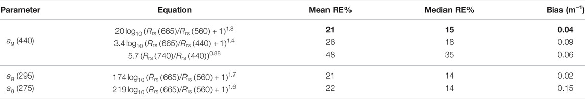
TABLE 1. Algorithms to retrieve a_g (440), a_g (295) and a_g (275), with associated performance metrics. Numbers in bold font highlight the best model.

For comparison, we tested the recently published so-called end-members approach of Houskeeper et al. (2021) with an algorithm based on the R_rs (665) to R_rs (440) ratio (Figure 5). These algorithms show a curvature starting at around a_g (440) values of 2 m⁻¹. An algorithm based on R_rs (740) to R_rs (440) ratio, the end-members of the MSI bands were also tested (Figure 5C). It shows a regional separation likely due to the use of reflectance at 740 nm, and did not prove to have a better accuracy even when fitting the model for the EGSL and JB independently (result not shown). In addition, R_rs (740) estimated from COPS (in the EGSL) is obtained using linear interpolation between 710 and 765 nm, while in JB it is measured using the HOCR, which could partly explain the regional differences.

In the EGSL and JB, respectively, 27 and 47% of the stations had values of a_g (440) > 2 m⁻¹, showing the necessity of an algorithm able to work in CDOM laden coastal waters. We found that the ratio of R_rs (665) to R_rs (560) gives results similar to the R_rs (665) to R_rs (440) ratio in terms of performance metrics, but with a slight curvature that is much less affected by this “saturation” at very high CDOM concentration. In terms of the mean and the median relative errors, R_rs (665) to R_rs (560) ratio yield values of 21 and 15%, respectively, for a range of a_g (440) values spanning from 0.16 to 11.5 m⁻¹, which is slightly better than that of the R_rs (665) to R_rs (440) ratio. Therefore, we chose the red-to-green band ratio algorithm for CDOM to process the satellite imagery because of the linearity of the relationship, the overall best retrieval performance relative to the other algorithm, and finally its weaker sensitivity to atmospheric correction errors (see below). We fitted this algorithm to retrieve CDOM in the UV-B domain, i.e. a_g (295) and a_g (275), which can be used to predict dissolved organic carbon (DOC) concentration in coastal waters (Fichot and Benner, 2011).

3.2.2 Suspended Particulate Matter Retrieval

Several empirical or semi-empirical algorithm formulas have been proposed to retrieve C_SPM from multispectral space-borne sensors in the literature (e.g., Dorji and Fearns, 2016; Tavora et al., 2020). In this study, we found that the best algorithm for C_SPM used a single reflectance at 740 nm (Figure 6), which is slightly better than 665 nm band used in many studies (e.g., Nechad et al. (2010) as shown in Figures 6A,B). The single red-band algorithm has good precision and accuracy in JB, with a bias of 0.30 mgL⁻¹ and a median RE of 27%. An outlier was found in optically shallow water, where the station depth was 0.56 m, which strongly influenced the Mean RE, degrading the algorithm’s overall performance. For the EGSL, we tested the algorithm published by Mohammadpour et al. (2015) based on the R_rs (710)/R_rs (665) ratio. It yields a slight degradation of the precision and accuracy metrics compared to those obtained using the single red-band algorithm with a median RE of 27% and a higher bias of 1.02 mgL⁻¹. Despite a better performance of the near infrared band algorithm (Table 2), we choose the red band algorithm as it is available on both OLI and MSI sensors, whereas 740 nm is only available on the later.

FIGURE 6

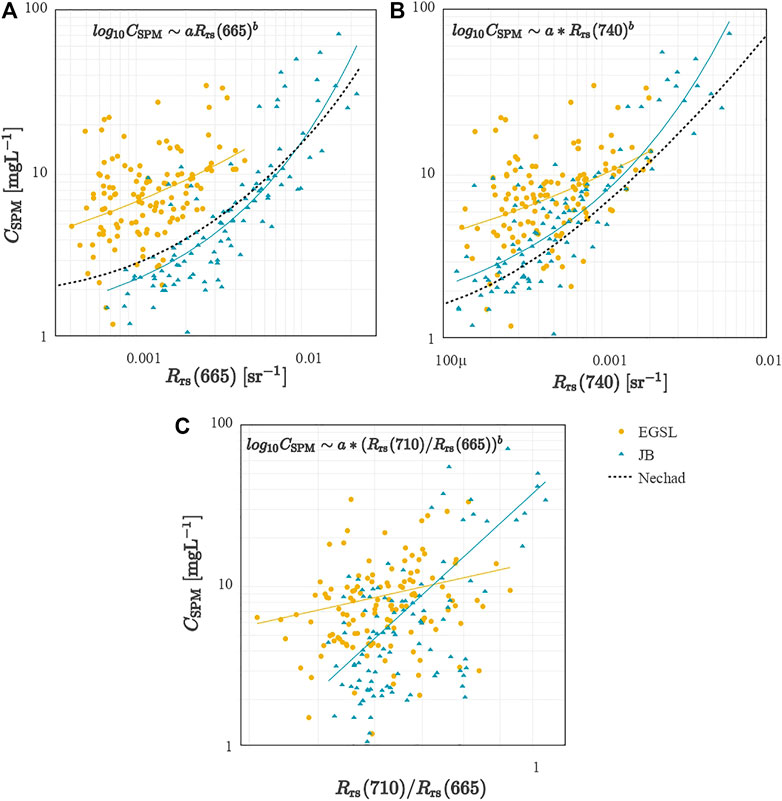
FIGURE 6. Regional empirical algorithms for C_SPM (A) from R_rs (665) (B) from R_rs (740), and (C) from R_rs (710)/R_rs (665) ratio. Dashed line corresponds to C_SPM values fitted with Nechad et al. (2010) semi-empirical algorithm.

TABLE 2

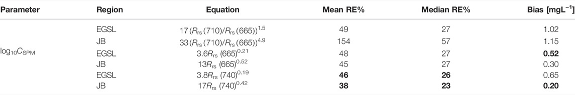
TABLE 2. Regional algorithms for C_SPM with their associated performance metrics. Numbers in bold font highlight the best model.

Residuals of the C_SPM empirical algorithm based on R_rs (665) show a positive correlation with a_g (440) (Figure 7). The slope is of 1.1 and 2.4 for the EGSL and JB, respectively, with p values significant for JB (p $<$ 0.001) but not for the EGSL (p = 0.023). Others band formulations (not presented here) have been tested with no better success.

FIGURE 7

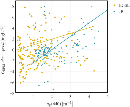
FIGURE 7. Residuals of the relationship between C_SPM and R_rs (665) (Figure 6A) as a function of a_g (440). Yellow dot represents data from the EGSL and blue represents triangle data from JB. Yellow and blue lines represents the linear regression between the residuals and a_g (440) with correlation coefficients (r) of 0.02 (p $<$ 0.05) and 0.17 (p $<$ 0.001) for the EGSL and JB, respectively.

3.3 Validation With Matching Satellite Imagery

The above algorithms were applied to actual satellite imagery from OLI and MSI after the application of atmospheric corrections (AC), which is a crucial pre-processing step for any aquatic applications. Therefore, we performed a matchup analysis for the entire database with the MSI and OLI sensors. As mentioned in the methods, we tested six atmospheric correction algorithms: 1) C2RCC, 2) C2X, 3) ACOLITE, 4) SeaDAS, 5) SSP, and 6) iCOR. Primarily, we will assess the performance of AC based on retrieved R_rs. The sensitivity of the a_g (440) and C_SPM retrievals to error in the R_rs retrieval introduced by the AC algorithm is then presented. For C_SPM, the single-band algorithm based on 665 nm available on both the MSI and OLI was chosen. It is noted that we parameterized the algorithms presented above by computing the coefficients for the specific satellite sensor bands of OLI and MSI, but also for other commonly used satellite sensors for coastal water monitoring (MODIS, MERIS, and OLCI). Those bands were retrieved from in situ R_rs through the RSR function of each sensor as provided by the space agencies. The regional empirical coefficients can be found in Supplementary Table S3.

3.3.1 R_rs Matchups

Figure 8 show the in situ versus remotely retrieved R_rs by the OLI and the MSI for each atmospheric correction algorithm. All the metrics for R_rs retrieval by wavelength and AC algorithm’s can be found in supplementary materials, Supplementary Table S1 for MSI and Supplementary Table S2 for OLI. The determination coefficient (R²) and the median symmetric accuracy (MdSA) are shown in Figure 9 to graphically represent the performance of R_rs retrieval for each sensor, AC algorithms, and wavelengths. In general, the algorithms tend to overestimate R_rs, except for C2RCC and C2X. In the same way, all algorithms except C2RCC and C2X overestimated R_rs at 443 and 740 nm, two wavelengths were in situ R_rs is at the lowest. For example, at 443 nm ACOLITE and iCOR give an SSPB of 1,243% and 1,417%, respectively, for the MSI, 342 and 471% for the OLI, indicating systematic overestimation. The green band is the most accurately retrieved by all algorithms, where R_rs is the highest. No single algorithm is found to give the best results for all wavelengths and sensors. At 443, 560, 665, 704, and 740 nm C2RCC get the more percent wins followed by C2X. C2RCC and C2X give an MdSA of 68 and 61%, respectively for the MSI green band (560 nm). Interestingly, SeaDAS give the best results for the OLI green band (561 nm) with an MdSA of 26%, closely followed by SSP with a MdSA of 34%. In contrast for the MSI green band (560 nm), SeaDAS and SSP gives an MdSA of 217 and 205%, respectively, while C2RCC and C2X give an MdSA of 40 and 47%, respectively for the OLI green band. Likewise, C2RCC and C2X give the lowest MdSA for the MSI red band (665 nm) with respectively 57 and 78%, while they give high MdSA for the OLI red band (655 nm) with 102 and 211%, respectively. Again inversely, SeaDAS and SSP give the lowest MdSA for the OLI red band (655 nm) with respectively 37 and 49%, while they give high MdSA for the MSI red band (665 nm) with 180 and 104%, respectively.

FIGURE 8

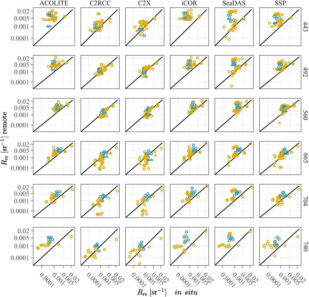
FIGURE 8. R_rs measured in situ and remotely in the EGSL (yellow) and in JB (blue) by MSI (circle) and OLI (triangle) in the blue (443 and 482, 492 nm, respectively), green (560, 561 nm, respectively), red (665, 655 nm, respectively), and NIR (704, 740 nm, MSI only) bands. The solid black line represents the 1:1 relation.

FIGURE 9

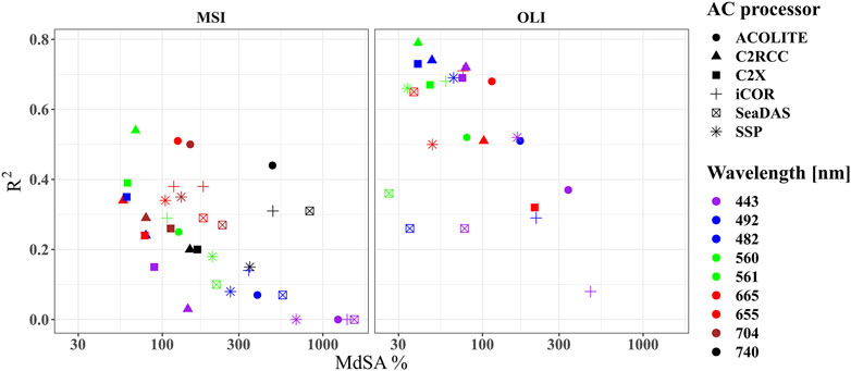
FIGURE 9. Performance metrics, y-axis coefficient of determination, and x-axis median symmetric accuracy, of atmospheric correction processors.

3.3.2 Colored Dissolved Organic Matter Matchup

The CDOM empirical algorithm based on the red-to-blue ratio [R_rs (665)/R_rs (440)] shows an important underestimation with all atmospheric corrections (Supplementary Figure S1; Table 3). The ACOLITE and iCOR showed very small dynamic range in terms of CDOM retrieval with all (but one for ACOLITE) a_g values $<$1 m⁻¹. The C2X algorithm, which performs better in highly absorptive waters, is able to detect a larger dynamic range for a_g with a slope closer to 1:1, but still systematically underestimates a_g (440) with a SSPB of -51%. This underestimation comes from the constant overestimation by atmospheric correction of R_rs in the blue part of the spectrum from satellite remote sensing.

TABLE 3

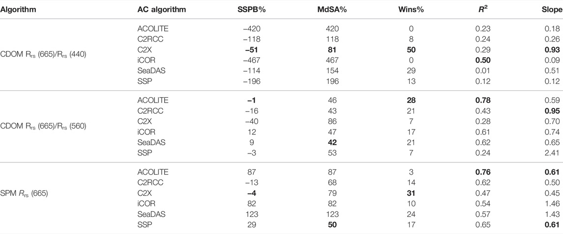
TABLE 3. Performance metrics of atmospheric correction algorithms for CDOM and SPM retrieval. For CDOM, only the algorithms for a_g (440) were tested (first two lines in Table 1). Numbers in bold font highlight the best atmospheric correction.

The use of a red/green reflectance ratio significantly improved CDOM retrieval for all AC algorithms (Figure 10; Table 3). For example, iCOR and ACOLITE respectively have small positive and negative SSPB of 12% and −1%, an MdSA of 47 and 45% respectively. A relatively strong linear relationship indicated by a R² of 0.78, is also observed for ACOLITE, suggesting a good preservation of the spatial pattern of CDOM. Therefore, ACOLITE errors seem less random and more systematic. Similarly, C2RCC, SSP, and SeaDAS also perform better for a_g (440) retrieval using the red-to-green band ratio. SeaDAS showed the lowest MdSA (42 versus 43% and 53% for C2RCC and SSP, respectively), while C2RCC showed the closest relation to the 1:1 line. SeaDAS points are, however, less dispersed than C2RCC, with an R² of 0.62 and 0.43, respectively.

FIGURE 10

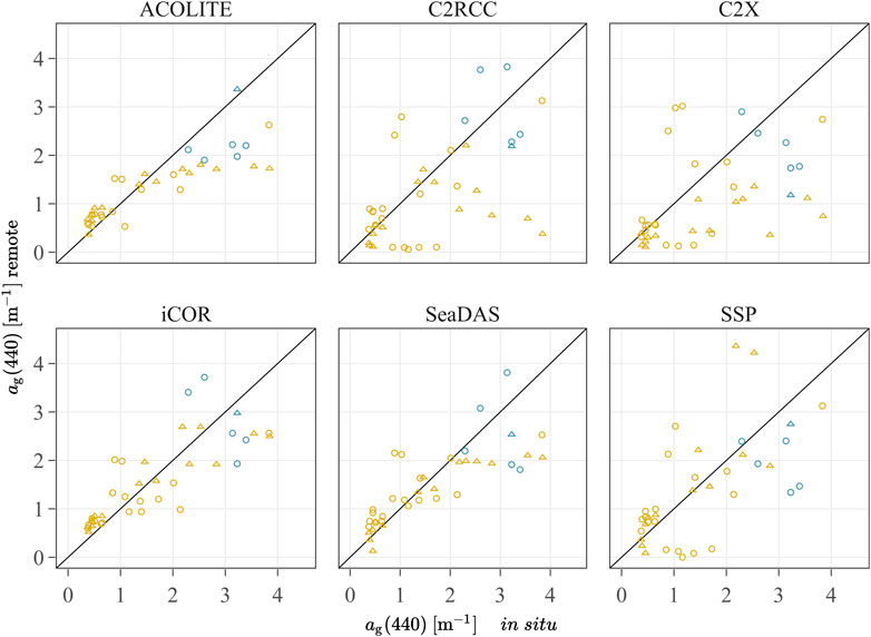
FIGURE 10. a_g (440) measured in situ vs. estimated remotely with the R_rs (665)/R_rs (560) empirical algorithm applied to MSI (circle) and OLI (triangle) in the EGSL (orange) and JB (blue). The solid black line represents the 1:1 relation.

3.3.3 Suspended Particulate Matter Matchup

As expected, C_SPM retrieval from the single-band empirical algorithm of the EGSL (Figure 11) is challenging due to large mass-specific IOP variability of SPM in this region (Figures 4, 6). Those results also show that for the limited matchup points available in JB, all are equally distributed with the EGSL data. This may tell that when it comes to satellite remote sensing, the better precision and accuracy of the C_SPM model in JB is lost. Our range of observation span from 2.11 to 36.40 (mgL⁻¹), but all except one observation are made below 10 (mgL⁻¹). ACOLITE, iCOR, SeaDAS, and SSP show a consistent overestimation of C_SPM, as it did for the R_rs retrieval. Consistently, SSP performed better than ACOLITE, iCOR, and SeaDAS with an SSPB more than twice lower with 29 versus 87, 82, and 123%, respectively.

FIGURE 11

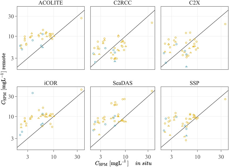
FIGURE 11. C_SPM measured in situ vs. estimated remotely with the red band empirical algorithm applied to MSI (circle) and OLI (triangle) in the EGSL (orange) and JB (blue). The solid black line represents the 1:1 relation.

4 Discussion

Our primary goal in this study was to provide empirical remote sensing algorithms to retrieve SPM and CDOM in Québec coastal waters from high-resolution multispectral satellite sensors (e.g., OLI and MSI). As shown in Figure 12, the spatial patterns follow the expected distribution of SPM and CDOM in the Bay of Sept–Iles area, where higher concentrations were found at the mouth of the main rivers (Moisie, Rapides, and Foin) at the time of the spring freshet (Araújo and Bélanger, 2022). We focused our study on the retrieval of CDOM and SPM because they are the main drivers of the coastal water color in our study area (Araújo and Bélanger, 2022). An empirical algorithm based on band ratios was preferred for CDOM over SAAs semi-analytical algorithms for their simplicity and because they are less sensitive to the absolute values of R_rs. In addition, Landsat and Sentinel-2 offer a limited number of spectral bands (relatively broad bands) in the visibility range, limiting the spectral inversion of R_rs. Moreover, SAAs semi-analytical algorithms are more sensitive to atmospheric correction errors than empirical algorithms based on band ratios. For CDOM, this has been achieved with a unique band ratio algorithm and a good level of confidence in both coastal regions. The range of CDOM recorded in Québec coastal waters is similar to other boreal environment such as the Baltic Sea (Kowalczuk et al., 2006; Berthon and Zibordi, 2010; Kratzer and Moore, 2018). In these dark and optically complex waters, it is difficult to accurately link other OACs with radiometric quantities such as chlorophyll-a, which makes a weak contribution to the total inherent optical properties (Araújo and Bélanger, 2022). A single red band algorithm for the SPM retrieval was chosen following Nechad et al. (2010). We found a satisfactory level of confidence for the James Bay region, considering the performance metrics of this specific algorithm. However, the EGSL region appears to be markedly different. The differences among the regions, their probable origin, and their consequences in terms of algorithm performance are discussed in the following sections.

FIGURE 12

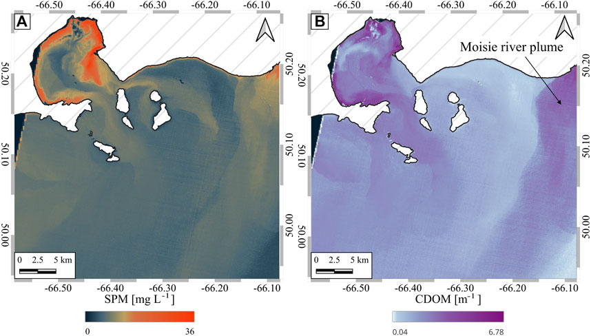
FIGURE 12. Map of SPM (A) and CDOM (B) in the Sept-Îles bay retrieved from the 17/05/2017 Sentinel-2 MSI image after atmospheric correction with the C2RCC processor.

4.1 Effects of Colored Dissolved Organic Matter and Suspended Particulate Matter on R_rs

The spectral relation of C_SPM, a_g (440), and R_rs (Figures 3A,C) shows that as we shift from lower wavelengths toward longer wavelengths, the relative influence of OACs on R_rs shifts from CDOM to SPM. The partition occurs between 560 and 665 nm. Empirical algorithms linking R_rs with a_g (440) and C_SPM take advantage of opposed physical properties, respectively absorption and scattering. Therefore, those two OACs are expected to act against one another in their effect on R_rs. CDOM mainly impacts R_rs by absorbing light in lower wavelengths and is generally considered negligible in longer wavelengths. However, our results show that at 665 nm, a_g is significant enough to affect C_SPM retrieval (Figure 7). In fact, the residuals of the C_SPM algorithm using R_rs (665) are positively correlated with a_g (440) (spearman correlation coefficient of 0.02 and 0.17 for EGSL and JB, respectively). The overestimation is associated with low CDOM concentration, and as a_g (440) increases, the relation shifts toward underestimation. As C_SPM and R_rs relation is positive, it indicates that CDOM absorption masks a part of the SPM signal at least up to 665 nm. This effect is of greater amplitude at 560 nm where absorption by CDOM and backscattering by SPM, acting against one another, is best seen. Consequently, R_rs (560) is not the best-suited reflectance to retrieve C_SPM because it needs prior retrieval of CDOM concentration to correct its effect. Contrary to this confounding effect, C_SPM has not shown any impact on a_g (440) retrieval, neither from the R_rs (665)/R_rs (440) nor the R_rs (665)/R_rs (560) algorithms. This is a surprising result, at least for the R_rs (665)/R_rs (560) residuals, considering that R_rs (560) seems to be under the equal influence of SPM and CDOM and that R_rs (665) is directly related to C_SPM. Yet, all results indicate that a_g (440) can be retrieved with an uncertainty as good as ∼18% from the R_rs (665)/R_rs (560) algorithm in the range from 0.16 to 11.5 m⁻¹ without any confounding effect coming from SPM.

The positive correlation between CDOM and R_rs at 665 nm (Figure 3C), yield a spearman correlation coefficient of 0.35 and 0.43 (p $<$ 0.001), for the EGSL and the JB, respectively. As we previously stated, the SPM backscattering effect is more significant than CDOM absorption at long wavelengths. In addition, we observed a positive correlation between C_SPM and CDOM (R² 0.34 and 0.55; p $<$ 0.001 for the EGSl and the JB, respectively), which further strengthens the relationship between a_g (440) and the R_rs (665)/R_rs (560) band ratio.

4.2 Linking R_rs Ratio and a_g (440)

The recently published end member approach (Hooker et al., 2020; Houskeeper et al., 2021) showed good results to retrieve CDOM concentration for a wide different range of water types. These authors argue that CDOM absorption can be retrieved using the ${[L_{\text{w}}]}_{\text{N}}$ ratio of UV to NIR bands, if available, or the extremity of the visible spectral range (e.g., 412 and 670 nm). Due to the limited number of bands on satellite sensors targeted in this study (MSI and OLI), the shortest wavelength available in the blue is 440 nm, but red (665) and NIR (740) bands are available for MSI. The end member approach shows good results with our dataset for the lower range of CDOM. In fact, we observed a strong linearity between a_g (440) and R_rs (665)/R_rs (440) in the log-space for a_g (440) below 2 m⁻¹. Above this value, however, a saturation of the algorithm starts to occur, as the ratio R_rs (665)/R_rs (440) tends to reach a plateau. Houskeeper et al. (2021) did not observed this saturation likely because the upper limit of their a_g (440) range was below 2 m⁻¹. The saturation may be explained by the fact that as CDOM concentration increases, the marine reflectance signal at 440 nm will reach an asymptotic value toward zero, hence the R_rs (440) variability become less and less significant in respect to the increase of CDOM concentration, resulting in a slope that will also tend toward zero. In our study area, a_g (440) the range from 0.16 to 11.5 m⁻¹ with a large number of observations with value $>$ 2 m⁻¹. In the upper range, we found a remarkable linear relationship between a_g (440) and the red-to-green ratio.

As the original work of Houskeeper et al. (2021) presented the R_rs (740)/R_rs (440) ratio, we chose to also present it under the same form. Our results show that CDOM in the EGSL and in JB cannot be retrieved directly and simultaneously for both environments as a regional separation appears in the relation of a_g (440) with this reflectance ratio. Our results also show no significant regional differences in the nature of CDOM. In fact, the CDOM spectral shapes between the two regions were not statistically different, with a spectral slope calculated for 350–500 nm spectral range of 0.0175 ± 0.0006 and 0.0167 ± 0.0010 nm⁻¹ for JB and EGSL, respectively. These spectral slopes are typical of coastal environments influenced by terrigenous input of CDOM (Babin et al., 2003). This mean that the regional separation of a_g (440) in relation with R_rs (740)/R_rs (440) is likely to come from the confounding effect of different regions $b_{\text{bp}}^{\ast \mathrm{S}\mathrm{P}\mathrm{M}}$.

Interestingly, CDOM matchup analysis brings forward the advantage of using algorithms based on the red-to-green band ratio, which is less sensitive to atmospheric correction errors (Figure 10). As noted in the matchup analysis, a significant underestimation error is associated with using R_rs in the blue, as atmospheric correction algorithms tend to overestimate R_rs in these wavelengths. Furthermore, performance metrics show that there is no significant difference among the CDOM algorithms using R_rs (665)/R_rs (440) and R_rs (665)/R_rs (560) when applied to in situ data. The assumption that CDOM absorption variability has a more pronounced impact on the remote sensing reflectance in the UV or in the blue wavelengths does not hold in these CDOM-rich nearshore waters. In this water type, the CDOM absorption actually reduced the variability of R_rs (443), and had a greater impact on R_rs (560). These results confirm several other studies that have put forward the use of red-to-green ratio to estimate CDOM concentration (Kutser et al., 2005; Ficek et al., 2011; Odermatt et al., 2012; Zhu et al., 2014; Zhang et al., 2021). Considering these points, the R_rs (665)/R_rs (560) algorithm should be used in the nearshore waters of EGSL and JB to provide accurate measurements of a_g (440). Similar results were obtained in northern inland waters: Boreal Lake of Europe (Kutser et al., 2005, 2012); lakes of the Yamal Peninsula, Russia (Dvornikov et al., 2018); and lakes of Minnesota, US (Brezonik et al., 2005, 2015; Menken et al., 2006; Olmanson et al., 2016). The upper limit of our red-to-green algorithm may be even higher, but more data would be needed to test the abovementioned relationship a_g (440) > 2 m⁻¹, which is expected to be more common in lakes (Kutser et al., 2005; Menken et al., 2006; Zhu et al., 2014; Brezonik et al., 2015; Olmanson et al., 2016; Zhang et al., 2021) than in coastal waters (e.g., Babin et al., 2003; Mannino et al., 2014).

4.3 Linking C_SPM and R_rs

The C_SPM relationship with R_rs is different between the EGSL and JB. In JB, this relationship is strong enough to derive an acceptable model for C_SPM from R_rs. The physical quantity $b_{\text{bp}}^{\ast \mathrm{S}\mathrm{P}\mathrm{M}}$, required for this regression to be accurate, is sufficiently constant as shown by Figure 7A. The semi-analytical approach proposed by Nechad et al. (2010) gives results similar to those that we proposed for JB and thus shows that this kind of algorithm is appropriate for this environment. In the EGSL, however, the $b_{\text{bp}}^{\ast \mathrm{S}\mathrm{P}\mathrm{M}}$ varies widely with C_SPM. The difference of $b_{\text{bp}}^{\ast \mathrm{S}\mathrm{P}\mathrm{M}}$ between the EGSL and JB may be explained by the mineralogical composition of SPM, the adsorption of organic matter, as well as by the type of flocs encountered. In particular, the particles encountered in the EGSL have very low backscattering efficiency compared to other coastal regions (Neukermans et al., 2012a), most likely due to large organic fraction (Araújo and Bélanger, 2022). Mohammadpour et al. (2017) reported values of 0.1 m² g for the total mass-specific scattering coefficient of SPM $(b_{\text{p}}^{\ast \mathrm{S}\mathrm{P}\mathrm{M}})$ in the lower estuary of St. Lawrence, which is in the same range as the values reported here assuming a backscattering to scattering ratio of 1.8%. In contrast, $b_{\text{bp}}^{\ast \mathrm{S}\mathrm{P}\mathrm{M}}$ of JB (0.014 m²g⁻¹) are closer to the values reported for mineral particles (Neukermans et al., 2012a; Reynolds et al., 2016). As pointed out by Nechad et al. (2010), most remote sensing algorithms assume no variability in $b_{\text{bp}}^{\ast \mathrm{S}\mathrm{P}\mathrm{M}}$. Our results show that such assumption is not met for the coastal waters of the EGSL. In fact the water masses of this region are stratified (Saucier et al., 2003), with upwelling zones and river plumes that can have a considerable effect in the coastal area. Seasonal variability in the distribution and stratification of those water masses could also give a sensible explanation for the observed variability of $b_{\text{bp}}^{\ast \mathrm{S}\mathrm{P}\mathrm{M}}$.

Band ratio algorithms to retrieve C_SPM have been used successfully in turbid estuaries (Doxaran et al., 2002, 2005). Previous studies conducted in the EGSL (Larouche and Boyer–Villemaire, 2010; Montes–Hugo et al., 2012; Montes–Hugo and Mohammadpour, 2012, 2013; Mohammadpour et al., 2015, 2017; Mohammadpour, 2016) have shown the difficulty to build solid empirical algorithms for C_SPM in these CDOM-rich waters. C_SPM algorithms for the EGSL have been previously developed and published in Montes–Hugo et al. (2012) and in Larouche and Boyer–Villemaire (2010), while Mohammadpour et al. (2015) proposed an algorithm for the maximum turbidity zone of the St. Lawrence estuary. Unlike the finding of Montes–Hugo et al. (2012) who used the band ratio of R_rs (670)/R_rs (560) as a proxy of C_SPM in the lower St. Lawrence estuary, the red-to-green ratio yield poor performance in our dataset (result not shown). Mohammadpour et al. (2015) published a power-law algorithm for C_SPM as a function of R_rs (708)/R_rs (665) and reported an r² of 0.687. We tested their formula they proposed, and obtained a Mean RE of 49 and 154% for the EGSL and JB, respectively, which was not considered to be satisfying. In fact, this low accuracy is well represented in Figure 6C as the data points are widely dispersed.

The interrelation of different optically active constituents and their effects on marine reflectance bring non-uniqueness in the solution to the inverse modeling of ocean color. It has been shown by Defoin-Platel and Chami (2007) that a significant part of inversion error in optically complex coastal waters originates from the non-uniqueness of the solution. Considering the high level of variability observed with the R_rs versus C_SPM relation in the EGSL, it is likely that the single band or band ratio algorithms suffers from this kind of error. To reduce such ambiguity, it is necessary to use as much spectral information as is available in terms of shape and magnitude. In fact, single band algorithms used only the magnitude of the reflectance at a single wavelength, while the band ratio algorithms destroy the magnitude information to keep only a small part of the spectral shape.

Considering the low efficiency of particulate backscattering specific to concentration in the EGSL (Araújo and Bélanger, 2022), even in relatively low CDOM concentration and even at 665 nm, a_g may have a significant effect on R_rs with respect to the b_bp. As the b_bp is the physical process allowing the use of R_rs as a direct proxy of C_SPM, it may provide an explanation for the poor result of the C_SPM algorithm in the EGSL.

4.4 Matchup Analysis and Atmospheric Correction Comparison

The matchup analysis has shown that the six atmospheric correction algorithms performed differently in terms of R_rs, a_g (440) and C_SPM retrieval. No algorithm is found to give the best performance for every target product. Both ends of the visible spectrum were the most difficult to accurately retrieve, as it approaches null reflectance due to the high absorption in the water column.

For 443 nm, Pahlevan et al. (2021) report that iCOR gives the best results for water types dominated by CDOM. In our analysis, it is the algorithm giving the largest error with an SSPB of 993.08%. Instead it is C2X, a version of the C2RCC neural network trained for extremely absorptive water that gives the best results. This could be expected as the coastal water of Québec, specifically the North Coast and JB are most often loaded with CDOM that absorbs most of the blue radiation. Considering this difficulty in front of which all other algorithms failed, C2X shows a relatively good performance at retrieving a_g (440) from the red/blue ratio. In fact, C2X MdSA for CDOM retrieval from the red/blue ratio is 81.49% slightly lower and close to the MdSA of 84.63% for R_rs (443) retrieval. However, the C2X gives error similar to the red/green and the red/blue algorithm, showing its limits as an algorithm useful in extreme cases. The CDOM red/green algorithms show better performance with ACOLITE algorithm, with the distribution of the point clearly representing the quasi null systematic error of the retrieval (SSPB of −1.40%). This may indicate that ACOLITE better preserves the spectral shape of R_rs in the green/red part of the spectrum. We also found the SeaDAS and SSP algorithms yielded better retrievals for OLI compared to MSI, consistent with the findings of Pahlevan et al. (2021).

The single red band algorithm for C_SPM shows a wide error for each atmospheric correction algorithm compared (Table 3). This may be directly related to the poor performance of the C_SPM algorithm tested with the in situ data, and may not represent the remote sensing retrieval performance. However, as the C_SPM algorithm is based on a single band in the red, the remote sensing errors can be directly related to the R_rs retrieval errors and the algorithm uncertainty itself. Therefore, the use of a fit for purpose atmospheric correction may be a suitable choice to apply this algorithm Pahlevan et al. (2021). With the least MdSA ($<$80%) and an acceptable bias ($<$20%), the neural nets (C2RCC and C2X) and SSP algorithms seem to be appropriate choices.

5 Conclusion

We developed empirical algorithms to retrieve C_SPM and a_g (440) in the coastal waters of Québec, dominated by high concentration of terrigenous CDOM from boreal watersheds. However, the retrieval of C_SPM in nearshore waters of the northern EGSL has shown the challenges to empirically link the concentration of this constituent with the optical properties. SPM is a generic term covering a wide diversity of particles assemblage, mineralogy, organic content, or flocs. Here, we only characterized SPM in terms of concentration (C) of total dry mass, as well as its inorganic/organic fractions. Acquiring information more specific to the SPM composition such as the mineralogy, the particle size distribution, as well as microphotography of particles and flocs would help to identify the specific variability observed in the nearshore EGSL. Furthermore, the methodology limitation in terms of C_SPM measurement (i.e. gravimetric method) and possible alternative or complementary methods such as counting the particles size distribution, would greatly help us to improve our understanding of this subject. In this article, we only presented simple empirical formulation to relate C_SPM to R_rs. The main findings and conclusions of this study can be summarized as follows.

Based in in situ observations a_g (440) is similarly related to R_rs (665)/R_rs (440) or R_rs (665)/R_rs (560) band ratio algorithms for the range 0.16–11.5 m⁻¹.

a_g (440), however, is best retrieved by the R_rs (665)/R_rs (560) algorithm when estimated using space-borne sensors such as the OLI and MSI due to lower error in R_rs retrieval in these bands after atmospheric correction. In our study area, ACOLITE dark fitting algorithm yielded the best a_g (440) retrievals for the range 0.38–3.84 m⁻¹.

C_SPM can be efficiently retrieved in eastern nearshore coastal waters of James Bay with a red single band algorithm.

C_SPM in the EGSL can neither be precisely retrieved from R_rs nor from b_bp due to a large variability in mass-specific IOPs due to the heterogeneous nature of SPM in this region, and to some extent, due to the confounding effects of CDOM in these dark waters. Clues have been given by the positive correlation of a_g (440) and b_b (532) indicating that very small particles ($<$ 0.2 µm) may be the missing component, invisibly increasing b_bp.

Characterization of SPM in terms of mineralogy, particle size distribution, and chemical analysis of the organic fraction would be the necessary steps to understand the variability of the $b_{\text{bp}}^{\ast \mathrm{S}\mathrm{P}\mathrm{M}}$ in the EGSL.

Data Availability Statement

The original contributions presented in the study are included in the article/Supplementary Material; further inquiries can be directed to the corresponding authors.

Author Contributions

RM contributed to data processing (C-OPS, SPM, atmospheric correction of satellite imagery), was responsible for algorithms development and the validation of satellite imagery, and he wrote the original draft of this manuscript. CASA contributed to the data processing (CDOM, backscattering) and revised the manuscript. RKS contributed to the atmospheric correction of satellite imagery and revised the manuscript. SB provided the original idea, and supervised the work, and he contributed to the data processing (HOCR) and revised the manuscript.

Funding

Funding for the collection of data used in this study come from three interdisciplinary projects: the Canadian Healthy Oceans Network (CHONe-II), funded by the Natural Sciences and Engineering Research Council of Canada (NSERC) in partnership with Fisheries and Ocean Canada and INREST (representing the Port of Sept-Îles and City of Sept-Îles); the WISE-Man Project (WaterSat Imaging Spectrometer Experiment (WISE) for Optically Shallow Inland and Coastal Waters Assessment), funded by the Canadian Space Agency through the Flights and Fieldwork for the Advancement of Science and Technology (FAST; FARIMA18) program and Fisheries and Oceans Canada through the Coastal Environmental Baseline Program; the COast-JB project (Coastal Oceanography of Eastern James Bay) funded by the Niskamoon corporation. CASA received a Ph.D. scholarship from the Fonds de Recherche du Québec-Nature et technologies (FRQNT, PBEEE grant number 263427). RKS is supported by a grant from the Belmont-Forum Biodiversa through the FRQNT (ACCES project). This study was also supported by the SB NSERC discovery grant (RGPIN-2019-06070).

Conflict of Interest

The authors declare that the research was conducted in the absence of any commercial or financial relationships that could be construed as a potential conflict of interest.

Publisher’s Note

All claims expressed in this article are solely those of the authors and do not necessarily represent those of their affiliated organizations, or those of the publisher, the editors and the reviewers. Any product that may be evaluated in this article, or claim that may be made by its manufacturer, is not guaranteed or endorsed by the publisher.

Acknowledgments

Special thanks to Dr. François Danhiez and Virginie Galindo for the fieldwork coordination of WISE-Man and CoastJB projects, respectively. The authors are also grateful to all the persons who contributed to the data collection on field, the students, professors, and captains of the ships used in the James Bay and the Estuary and Gulf of St. Lawrence. We thank Drs Gege and Wang for their constructive comments.

Supplementary Material

The Supplementary Material for this article can be found online at: https://www.frontiersin.org/articles/10.3389/frsen.2022.834908/full#supplementary-material

References

Antoine, D., Hooker, S. B., Bélanger, S., Matsuoka, A., and Babin, M. (2013). Apparent Optical Properties of the Canadian Beaufort Sea - Part 1: Observational Overview and Water Column Relationships. Biogeosciences 10, 4493–4509. doi:10.5194/bg-10-4493-2013

CrossRef Full Text | Google Scholar

Araújo, C. A. S., and Bélanger, S. (2022). Variability of Bio-Optical Properties in Nearshore Waters of the Estuary and Gulf of St. Lawrence: Absorption and Backscattering Coefficients. Estuarine, Coastal Shelf Sci. 264, 107688. doi:10.1016/j.ecss.2021.107688

CrossRef Full Text | Google Scholar

Aurin, D., Mannino, A., and Franz, B. (2013). Spatially Resolving Ocean Color and Sediment Dispersion in River Plumes, Coastal Systems, and continental Shelf Waters. Remote Sensing Environ. 137, 212–225. doi:10.1016/j.rse.2013.06.018

CrossRef Full Text | Google Scholar

Babin, M., Stramski, D., Ferrari, G. M., Claustre, H., Bricaud, A., Obolensky, G., et al. (2003). Variations in the Light Absorption Coefficients of Phytoplankton, Nonalgal Particles, and Dissolved Organic Matter in Coastal Waters Around Europe. J. Geophys. Res. 108, 882. doi:10.1029/2001JC000882

CrossRef Full Text | Google Scholar

Bélanger, S., Carrascal-Leal, C., Jaegler, T., Larouche, P., and Galbraith, P. (2017). Assessment of Radiometric Data from a Buoy in the St. Lawrence Estuary. J. Atmos. Oceanic Technol. 34, 877–896. doi:10.1175/JTECH-D-16-0176.1

CrossRef Full Text | Google Scholar

Berthon, J.-F., and Zibordi, G. (2010). Optically Black Waters in the Northern Baltic Sea. Geophys. Res. Lett. 37, a–n. doi:10.1029/2010GL043227

CrossRef Full Text | Google Scholar

Boss, E., Pegau, W. S., Lee, M., Twardowski, M., Shybanov, E., Korotaev, G., et al. (2004). Particulate Backscattering Ratio at LEO 15 and its Use to Study Particle Composition and Distribution. J. Geophys. Res. 109, 1514. doi:10.1029/2002JC001514

CrossRef Full Text | Google Scholar

Brezonik, P. L., Olmanson, L. G., Finlay, J. C., and Bauer, M. E. (2015). Factors Affecting the Measurement of Cdom by Remote Sensing of Optically Complex Inland Waters. Remote Sensing Environ. 157, 199–215. doi:10.1016/j.rse.2014.04.033

CrossRef Full Text | Google Scholar

Brezonik, P., Menken, K. D., and Bauer, M. (2005). Landsat-based Remote Sensing of Lake Water Quality Characteristics, Including Chlorophyll and Colored Dissolved Organic Matter (CDOM). Lake Reservoir Manage. 21, 373–382. doi:10.1080/07438140509354442

CrossRef Full Text | Google Scholar

Brockmann, C., Doerffer, R., Peters, M., Kerstin, S., Embacher, S., and Ruescas, A. (2016). Evolution of the C2RCC Neural Network for Sentinel 2 and 3 for the Retrieval of Ocean Colour Products in Normal and Extreme Optically Complex Waters. Living Planet. Symp. 740, 54.

Google Scholar

Chen, J., Zhu, W., Tian, Y. Q., and Yu, Q. (2020). Monitoring Dissolved Organic Carbon by Combining Landsat-8 and Sentinel-2 Satellites: Case Study in Saginaw River Estuary, Lake Huron. Sci. Total Environ. 718, 137374. doi:10.1016/j.scitotenv.2020.137374

PubMed Abstract | CrossRef Full Text | Google Scholar

Costoya, X., Fernández‐Nóvoa, D., deCastro, M., Santos, F., Lazure, P., and Gómez‐Gesteira, M. (2016). Modulation of Sea Surface Temperature Warming in the B Ay of B Iscay by L Oire and G Ironde R Ivers. J. Geophys. Res. Oceans 121, 966–979. doi:10.1002/2015JC011157

CrossRef Full Text | Google Scholar

Cyr, F., Bourgault, D., Galbraith, P. S., and Gosselin, M. (2015). Turbulent Nitrate Fluxes in the Lower St. Lawrence Estuary, Canada. J. Geophys. Res. Oceans 120, 2308–2330. doi:10.1002/2014JC010272

CrossRef Full Text | Google Scholar

[Dataset] Montes-Hugo, M., Roy, S., Gagne, J. P., Demers, S., Cizmeli, S., and Mas, S. (2012). Ocean Colour and Distribution of Suspended Particulates in the St. Lawrence Estuary. Quebec, Canada: Lawrence Estuary. doi:10.12760/01-2012-1-01

CrossRef Full Text | Google Scholar

De Keukelaere, L., Sterckx, S., Adriaensen, S., Knaeps, E., Reusen, I., Giardino, C., et al. (2018). Atmospheric Correction of Landsat-8/OLI and Sentinel-2/MSI Data Using iCOR Algorithm: Validation for Coastal and Inland Waters. Eur. J. Remote Sensing 51, 525–542. doi:10.1080/22797254.2018.1457937

CrossRef Full Text | Google Scholar

Defoin-Platel, M., and Chami, M. (2007). How Ambiguous Is the Inverse Problem of Ocean Color in Coastal Waters? J. Geophys. Res. 112, 3847. doi:10.1029/2006JC003847

CrossRef Full Text | Google Scholar

DFO (2009). Does Eelgrass (Zostera marina) Meet the Criteria as an Ecologically Significant Species? Tech. Rep. 018, DFO.

Google Scholar

Dorji, P., and Fearns, P. (2016). A Quantitative Comparison of Total Suspended Sediment Algorithms: A Case Study of the Last Decade for MODIS and Landsat-Based Sensors. Remote Sensing 8, 810. doi:10.3390/rs8100810

CrossRef Full Text | Google Scholar

Doxaran, D., Cherukuru, R. C. N., and Lavender, S. J. (2005). Use of Reflectance Band Ratios to Estimate Suspended and Dissolved Matter Concentrations in Estuarine Waters. Int. J. Remote Sensing 26, 1763–1769. doi:10.1080/01431160512331314092

CrossRef Full Text | Google Scholar

Doxaran, D., Froidefond, J.-M., Lavender, S., and Castaing, P. (2002). Spectral Signature of Highly Turbid Waters Application with SPOT Data to Quantify Suspended Particulate Matter Concentrations. Remote Sensing Environ. 81, 149. doi:10.1016/S0034-4257(01)00341-8

CrossRef Full Text | Google Scholar

Doxaran, D., Leymarie, E., Nechad, B., Dogliotti, A., Ruddick, K., Gernez, P., et al. (2016). Improved Correction Methods for Field Measurements of Particulate Light Backscattering in Turbid Waters. Opt. Express 24, 3615–3637. doi:10.1364/OE.24.003615

PubMed Abstract | CrossRef Full Text | Google Scholar

Duarte, C. M. (1991). Seagrass Depth Limits. Aquat. Bot. 40, 363–377. doi:10.1016/0304-3770(91)90081-F

CrossRef Full Text | Google Scholar

Dvornikov, Y., Leibman, M., Heim, B., Bartsch, A., Herzschuh, U., Skorospekhova, T., et al. (2018). Terrestrial CDOM in Lakes of Yamal Peninsula: Connection to Lake and Lake Catchment Properties. Remote Sensing 10, 167. doi:10.3390/rs10020167

CrossRef Full Text | Google Scholar

Ficek, D., Zapadka, T., and Dera, J. (2011). Remote Sensing Reflectance of Pomeranian Lakes and the Baltic**The Study Was Partially Financed by MNiSW (Ministry of Science and Higher Education) as a Research Project N N306 066434 in the Years 2008-2011. The Partial Support for This Study Was Also provided by the SatBałtyk Project (Satellite Monitoring of the Baltic Sea Environment) Funded by the European Union from the European Regional Development Fund Contract No. POIG 01.01.02-22-011/09.the Paper Was Presented at the 6th International Conference 'Current Problems in the Optics of Natural Waters', St. Petersburg, Russia, 6-10 September 2011. Oceanologia 53, 959–970. doi:10.5697/oc.53-4.959

CrossRef Full Text | Google Scholar

Fichot, C. G., and Benner, R. (2011). A Novel Method to Estimate DOC Concentrations from CDOM Absorption Coefficients in Coastal Waters. Geophys. Res. Lett. 38, a–n. doi:10.1029/2010GL046152

CrossRef Full Text | Google Scholar

Franz, B. A., Bailey, S. W., Kuring, N., and Werdell, P. J. (2015). Ocean Color Measurements with the Operational Land Imager on Landsat-8: Implementation and Evaluation in SeaDAS. J. Appl. Remote Sens 9, 096070. doi:10.1117/1.JRS.9.096070

CrossRef Full Text | Google Scholar

Gitelson, A., Garbuzov, G., Szilagyi, F., Mittenzwey, K.-H., Karnieli, A., and Kaiser, A. (1993). Quantitative Remote Sensing Methods for Real-Time Monitoring of Inland Waters Quality. Int. J. Remote Sensing 14, 1269–1295. doi:10.1080/01431169308953956

CrossRef Full Text | Google Scholar

Gordon, H. R., and Ding, K. (1992). Self-shading of In-Water Optical Instruments. Limnol. Oceanogr. 37, 491–500. doi:10.4319/lo.1992.37.3.0491

CrossRef Full Text | Google Scholar

Gordon, H. R., and Wang, M. (1994). Retrieval of Water-Leaving Radiance and Aerosol Optical Thickness over the Oceans with SeaWiFS: a Preliminary Algorithm. Appl. Opt. 33, 443–452. doi:10.1364/ao.33.000443

PubMed Abstract | CrossRef Full Text | Google Scholar

Hooker, S. B., Matsuoka, A., Kudela, R. M., Yamashita, Y., Suzuki, K., and Houskeeper, H. F. (2020). A Global End-Member Approach to Derive aCDOM(440) from Near-Surface Optical Measurements. Biogeosciences 17, 475–497. doi:10.5194/bg-17-475-2020

CrossRef Full Text | Google Scholar

Hooker, S. B., Morrow, J. H., and Matsuoka, A. (2013). Apparent Optical Properties of the Canadian Beaufort Sea – Part 2: The 1% and 1 Cm Perspective in Deriving and Validating AOP Data Products. Biogeosciences 10, 4511–4527. doi:10.5194/bg-10-4511-2013

CrossRef Full Text | Google Scholar

Houskeeper, H. F., Hooker, S. B., and Kudela, R. M. (2021). Spectral Range within Global aCDOM(440) Algorithms for Oceanic, Coastal, and Inland Waters with Application to Airborne Measurements. Remote Sensing Environ. 253, 112155. doi:10.1016/j.rse.2020.112155

CrossRef Full Text | Google Scholar

Hudon, C., Gagnon, P., Rondeau, M., Hébert, S., Gilbert, D., Hill, B., et al. (2017). Hydrological and Biological Processes Modulate Carbon, Nitrogen and Phosphorus Flux from the St. Lawrence River to its Estuary (Quebec, Canada). Biogeochemistry 135, 251–276. doi:10.1007/s10533-017-0371-4

CrossRef Full Text | Google Scholar

IOCCG (2018). Ocean Optics and Biogeochemistry Protocols for Satellite Ocean Colour Sensor Validation; Volume 1.0. Inherent Optical Property Measurements and Protocols: Absorption Coefficient. Dartmouth, Canada: IOCCG, 78. doi:10.25607/OBP-119

CrossRef Full Text | Google Scholar

Kirk, J. T. O. (2011). Light and Photosynthesis in Aquatic Ecosystems. third edn. Cambridge: Cambridge University Press.

Google Scholar

Kowalczuk, P., A. Stedmon, C., and Markager, S. (2006). Modeling Absorption by CDOM in the Baltic Sea from Season, Salinity and Chlorophyll. Mar. Chem. 101, 1–11. doi:10.1016/j.marchem.2005.12.005

CrossRef Full Text | Google Scholar

Kratzer, S., and Moore, G. (2018). Inherent Optical Properties of the Baltic Sea in Comparison to Other Seas and Oceans. Remote Sensing 10, 418. doi:10.3390/rs10030418

CrossRef Full Text | Google Scholar

Kutser, T., Paavel, B., Verpoorter, C., Kauer, T., and Vahtmäe, E. (2012). Remote Sensing of Water Quality in Optically Complex Lakes. Int. Arch. Photogramm. Remote Sens. Spat. Inf. Sci. XXXIX-B8, 165–169. doi:10.5194/isprsarchives-XXXIX-B8-165-2012

CrossRef Full Text | Google Scholar

Kutser, T., Pierson, D. C., Tranvik, L., Reinart, A., Sobek, S., and Kallio, K. (2005). Using Satellite Remote Sensing to Estimate the Colored Dissolved Organic Matter Absorption Coefficient in Lakes. Ecosystems 8, 709–720. doi:10.1007/s10021-003-0148-6

CrossRef Full Text | Google Scholar

Larouche, P., and Boyer-Villemaire, U. (2010). Suspended Particulate Matter in the St. Lawrence Estuary and Gulf Surface Layer and Development of a Remote Sensing Algorithm. Estuarine, Coastal Shelf Sci. 90, 241–249. doi:10.1016/j.ecss.2010.09.005

CrossRef Full Text | Google Scholar

Le Fouest, V., Zakardjian, B., Saucier, F. J., and Çizmeli, S. A. (2006). Application of SeaWIFS- and AVHRR-Derived Data for Mesoscale and Regional Validation of a 3-D High-Resolution Physical-Biological Model of the Gulf of St. Lawrence (Canada). J. Mar. Syst. 60, 30–50. doi:10.1016/j.jmarsys.2005.11.008

CrossRef Full Text | Google Scholar

Li, P., Ke, Y., Bai, J., Zhang, S., Chen, M., and Zhou, D. (2019). Spatiotemporal Dynamics of Suspended Particulate Matter in the Yellow River Estuary, China during the Past Two Decades Based on Time-Series Landsat and Sentinel-2 Data. Mar. Pollut. Bull. 149, 110518. doi:10.1016/j.marpolbul.2019.110518

PubMed Abstract | CrossRef Full Text | Google Scholar

Mannino, A., Novak, M. G., Hooker, S. B., Hyde, K., and Aurin, D. (2014). Algorithm Development and Validation of CDOM Properties for Estuarine and continental Shelf Waters along the Northeastern U.S. Coast. Remote Sensing Environ. 152, 576–602. doi:10.1016/j.rse.2014.06.027

CrossRef Full Text | Google Scholar

Matthews, M. W. (2011). A Current Review of Empirical Procedures of Remote Sensing in Inland and Near-Coastal Transitional Waters. Int. J. Remote Sensing 32, 6855–6899. doi:10.1080/01431161.2010.512947

CrossRef Full Text | Google Scholar

Menken, K. D., Brezonik, P. L., and Bauer, M. E. (2006). Influence of Chlorophyll and Colored Dissolved Organic Matter (CDOM) on Lake Reflectance Spectra: Implications for Measuring Lake Properties by Remote Sensing. Lake Reservoir Manage. 22, 179–190. doi:10.1080/07438140609353895

CrossRef Full Text | Google Scholar

Mohammadpour, G., Gagné, J.-P., Larouche, P., and Montes-Hugo, M. A. (2017). Optical Properties of Size Fractions of Suspended Particulate Matter in Littoral Waters of Québec. Biogeosciences 14, 5297–5312. doi:10.5194/bg-14-5297-2017

CrossRef Full Text | Google Scholar

Mohammadpour, G., Montes-Hugo, M. A., Stavn, R., Gagné, J.-P., and Larouche, P. (2015). Particle Composition Effects on MERIS-Derived SPM: A Case Study in the Saint Lawrence Estuary. Can. J. Remote Sensing 41, 515–524. doi:10.1080/07038992.2015.1110012

CrossRef Full Text | Google Scholar

Mohammadpour, G. (2016). Remote Sensing of Suspended Particulate Matter Concentration in the St. Lawrence Estuary. Ph.D. thesis. Rimouski, Canada: UQAR-ISMER.

Montes-Hugo, M. A., and Mohammadpour, G. (2012). Biogeo-optical Modeling of SPM in the St. Lawrence Estuary. Can. J. Remote Sensing 38, 14. doi:10.5589/m12-033

CrossRef Full Text | Google Scholar

Montes-Hugo, M. A., and Mohammadpour, G. (2013). Satellite-derived Suspended Particulates in the Saint Lawrence Estuary: Uncertainties Due to Bottom Effects. Can. J. Remote Sensing 39, 444–454. doi:10.5589/m13-050

CrossRef Full Text | Google Scholar

Morley, S. K., Brito, T. V., and Welling, D. T. (2018). Measures of Model Performance Based on the Log Accuracy Ratio. Space Weather 16, 69–88. doi:10.1002/2017SW001669

CrossRef Full Text | Google Scholar

Morrow, J. H., Booth, C. R., and Lind, R. N. (2010). The Compact-Optical Profiling System (C-OPS), 16.

Google Scholar

Mueller, J. L., Fargion, G. S., McClain, C. R., Mueller, J. L., Bidigare, R. R., Trees, C., et al. (2003). Ocean Optics Protocols for Satellite Ocean Color Sensor Validation. Revision 5 (5), 43.

Google Scholar

Murphy, G. E. P., Dunic, J. C., Adamczyk, E. M., Bittick, S. J., Côté, I. M., Cristiani, J., et al. (2021). From Coast to Coast to Coast: Ecology and Management of Seagrass Ecosystems across Canada. FACETS 6, 139–179. doi:10.1139/facets-2020-0020

CrossRef Full Text | Google Scholar

Nechad, B., Ruddick, K. G., and Park, Y. (2010). Calibration and Validation of a Generic Multisensor Algorithm for Mapping of Total Suspended Matter in Turbid Waters. Remote Sensing Environ. 114, 854–866. doi:10.1016/j.rse.2009.11.022

CrossRef Full Text | Google Scholar

Neukermans, G., Loisel, H., Mériaux, X., Astoreca, R., and Mckee, D. (2012a). In Situ variability of Mass-specific Beam Attenuation and Backscattering of marine Particles with Respect to Particle Size, Density, and Composition. Limnol. Oceanogr. 57, 124–144. doi:10.4319/lo.2011.57.1.012410.4319/lo.2012.57.1.0124

CrossRef Full Text | Google Scholar

Neukermans, G., Ruddick, K., Loisel, H., and Roose, P. (2012b). Optimization and Quality Control of Suspended Particulate Matter Concentration Measurement Using Turbidity Measurements. Limnol. Oceanogr. Methods 10, 1011–1023. doi:10.4319/lom.2012.10.1011

CrossRef Full Text | Google Scholar

Normandin, C., Lubac, B., Sottolichio, A., Frappart, F., Ygorra, B., and Marieu, V. (2019). Analysis of Suspended Sediment Variability in a Large Highly Turbid Estuary Using a 5‐Year‐Long Remotely Sensed Data Archive at High Resolution. J. Geophys. Res. Oceans 124, 7661–7682. doi:10.1029/2019JC015417

CrossRef Full Text | Google Scholar

Odermatt, D., Gitelson, A., Brando, V. E., and Schaepman, M. (2012). Review of Constituent Retrieval in Optically Deep and Complex Waters from Satellite Imagery. Remote Sensing Environ. 118, 116–126. doi:10.1016/j.rse.2011.11.013

CrossRef Full Text | Google Scholar

Olmanson, L. G., Brezonik, P. L., Finlay, J. C., and Bauer, M. E. (2016). Comparison of Landsat 8 and Landsat 7 for Regional Measurements of CDOM and Water Clarity in Lakes. Remote Sensing Environ. 185, 119–128. doi:10.1016/j.rse.2016.01.007

CrossRef Full Text | Google Scholar

Osadchiev, A., and Sedakov, R. (2019). Spreading Dynamics of Small River Plumes off the Northeastern Coast of the Black Sea Observed by Landsat 8 and Sentinel-2. Remote Sensing Environ. 221, 522–533. doi:10.1016/j.rse.2018.11.043

CrossRef Full Text | Google Scholar

Pahlevan, N., Mangin, A., Balasubramanian, S. V., Smith, B., Alikas, K., Arai, K., et al. (2021). ACIX-aqua: A Global Assessment of Atmospheric Correction Methods for Landsat-8 and Sentinel-2 over Lakes, Rivers, and Coastal Waters. Remote Sensing Environ. 258, 112366. doi:10.1016/j.rse.2021.112366

CrossRef Full Text | Google Scholar

Pahlevan, N., Sarkar, S., Franz, B. A., Balasubramanian, S. V., and He, J. (2017). Sentinel-2 MultiSpectral Instrument (MSI) Data Processing for Aquatic Science Applications: Demonstrations and Validations. Remote Sensing Environ. 201, 47–56. doi:10.1016/j.rse.2017.08.033

CrossRef Full Text | Google Scholar

Reynolds, R. A., Stramski, D., and Neukermans, G. (2016). Optical Backscattering by Particles in Arctic Seawater and Relationships to Particle Mass Concentration, Size Distribution, and Bulk Composition. Limnol. Oceanogr. 61, 1869–1890. doi:10.1002/lno.10341

CrossRef Full Text | Google Scholar

Ruddick, K. G., Ovidio, F., and Rijkeboer, M. (2000). Atmospheric Correction of SeaWiFS Imagery for Turbid Coastal and Inland Waters. Appl. Opt. 39, 897–912. doi:10.1364/ao.39.000897

PubMed Abstract | CrossRef Full Text | Google Scholar

Saucier, F. J., Roy, F., Gilbert, D., Pellerin, P., and Ritchie, H. (2003). Modeling the Formation and Circulation Processes of Water Masses and Sea Ice in the Gulf of St. Lawrence, Canada. J. Geophys. Res. 108, 686. doi:10.1029/2000JC000686

CrossRef Full Text | Google Scholar

Seegers, B. N., Stumpf, R. P., Schaeffer, B. A., Loftin, K. A., and Werdell, P. J. (2018). Performance Metrics for the Assessment of Satellite Data Products: an Ocean Color Case Study. Opt. Express 26, 7404. doi:10.1364/OE.26.007404

PubMed Abstract | CrossRef Full Text | Google Scholar

Singh, R. K., Shanmugam, P., He, X., and Schroeder, T. (2019). UV-NIR Approach with Non-zero Water-Leaving Radiance Approximation for Atmospheric Correction of Satellite Imagery in Inland and Coastal Zones. Opt. Express 27, A1118. doi:10.1364/OE.27.0A1118

PubMed Abstract | CrossRef Full Text | Google Scholar

Tavora, J., Boss, E., Doxaran, D., and Hill, P. (2020). An Algorithm to Estimate Suspended Particulate Matter Concentrations and Associated Uncertainties from Remote Sensing Reflectance in Coastal Environments. Remote Sensing 12, 2172. doi:10.3390/rs12132172

CrossRef Full Text | Google Scholar

Therriault, J.-C., and Lacroix, G. (1976). Nutrients, Chlorophyll, and Internal Tides in the St. Lawrence Estuary. J. Fish. Board Can. 11, 326. doi:10.1139/f76-326

CrossRef Full Text | Google Scholar

van der Molen, J., Ruardij, P., and Greenwood, N. (2017). A 3D SPM Model for Biogeochemical Modelling, with Application to the Northwest European continental Shelf. J. Sea Res. 127, 63–81. doi:10.1016/j.seares.2016.12.003

CrossRef Full Text | Google Scholar

Vanhellemont, Q. (2019a). Adaptation of the Dark Spectrum Fitting Atmospheric Correction for Aquatic Applications of the Landsat and Sentinel-2 Archives. Remote Sensing Environ. 225, 175–192. doi:10.1016/j.rse.2019.03.010

CrossRef Full Text | Google Scholar

Vanhellemont, Q. (2019b). Daily Metre-Scale Mapping of Water Turbidity Using CubeSat Imagery. Opt. Express 27, A1372–A1399. doi:10.1364/OE.27.0A1372

PubMed Abstract | CrossRef Full Text | Google Scholar

Vanhellemont, Q., and Ruddick, K. (2018). Atmospheric Correction of Metre-Scale Optical Satellite Data for Inland and Coastal Water Applications. Remote Sensing Environ. 216, 586–597. doi:10.1016/j.rse.2018.07.015

CrossRef Full Text | Google Scholar

Vanhellemont, Q., and Ruddick, K. (2021). Atmospheric Correction of Sentinel-3/OLCI Data for Mapping of Suspended Particulate Matter and Chlorophyll-A Concentration in Belgian Turbid Coastal Waters. Remote Sensing Environ. 256, 112284. doi:10.1016/j.rse.2021.112284

CrossRef Full Text | Google Scholar

Vanhellemont, Q., and Ruddick, K. (2014). Turbid Wakes Associated with Offshore Wind Turbines Observed with Landsat 8. Remote Sensing Environ. 145, 105–115. doi:10.1016/j.rse.2014.01.009

CrossRef Full Text | Google Scholar

Vanhellemont, Q. (2020). Sensitivity Analysis of the Dark Spectrum Fitting Atmospheric Correction for Metre- and Decametre-Scale Satellite Imagery Using Autonomous Hyperspectral Radiometry. Opt. Express 28, 29948–29965. doi:10.1364/oe.397456

PubMed Abstract | CrossRef Full Text | Google Scholar

Zhang, Y., and Xie, H. (2015). Photomineralization and Photomethanification of Dissolved Organic Matter in Saguenay River Surface Water. Biogeosciences 12, 6823–6836. doi:10.5194/bg-12-6823-2015

CrossRef Full Text | Google Scholar

Zhang, Y., Zhou, L., Zhou, Y., Zhang, L., Yao, X., Shi, K., et al. (2021). Chromophoric Dissolved Organic Matter in Inland Waters: Present Knowledge and Future Challenges. Sci. Total Environ. 759, 143550. doi:10.1016/j.scitotenv.2020.143550

PubMed Abstract | CrossRef Full Text | Google Scholar

Zheng, G., and DiGiacomo, P. M. (2017). Uncertainties and Applications of Satellite-Derived Coastal Water Quality Products. Prog. Oceanography 159, 45–72. doi:10.1016/j.pocean.2017.08.007

CrossRef Full Text | Google Scholar

Zhu, W., Yu, Q., Tian, Y. Q., Becker, B. L., Zheng, T., and Carrick, H. J. (2014). An Assessment of Remote Sensing Algorithms for Colored Dissolved Organic Matter in Complex Freshwater Environments. Remote Sensing Environ. 140, 766–778. doi:10.1016/j.rse.2013.10.015

CrossRef Full Text | Google Scholar

Zibordi, G., and Ferrari, G. M. (1995). Instrument Self-Shading in Underwater Optical Measurements: Experimental Data. Appl. Opt. 34, 2750. doi:10.1364/AO.34.002750

PubMed Abstract | CrossRef Full Text | Google Scholar