
94% of researchers rate our articles as excellent or good
Learn more about the work of our research integrity team to safeguard the quality of each article we publish.
Find out more
ORIGINAL RESEARCH article
Front. Remote Sens., 12 April 2022
Sec. Atmospheric Remote Sensing
Volume 3 - 2022 | https://doi.org/10.3389/frsen.2022.833340
This article is part of the Research TopicDSCOVR EPIC/NISTAR: 5 years of Observing Earth from the first Lagrangian PointView all 24 articles
 Robert Frouin1*
 Jing Tan1
 Mathieu Compiègne2
 Didier Ramon2
 Marshall Sutton3
 Hiroshi Murakami4
 David Antoine5,6Uwe Send1
 Jeff Sevadjian1
 Vincenzo Vellucci6
The EPIC/DSCOVR observations of the Earth’s surface lit by the Sun made from the first Lagrange point several times during the day in spectral bands centered on 443, 551, and 680 nm are used to estimate daily mean photosynthetically available radiation (PAR) at the ice-free ocean surface. The PAR algorithm uses a budget approach, in which the solar irradiance reaching the surface is obtained by subtracting from the irradiance arriving at the top of the atmosphere (known), the irradiance reflected to space (estimated from the EPIC Level 1b radiance data), taking account of atmospheric transmission and surface albedo (modeled). Clear and cloudy regions within a pixel do not need to be distinguished, which dismisses the need for often-arbitrary assumptions about cloudiness distribution within a pixel and is therefore adapted to the relatively large EPIC pixels. A daily mean PAR is estimated on the source grid for each EPIC instantaneous daytime observation, assuming no cloudiness changes during the day, and the individual estimates are remapped and weight-averaged using the cosine of the Sun zenith angle. In the computations, wind speed, surface pressure, and water vapor amount are extracted from NCEP Reanalysis 2 data, aerosol optical thickness and Angström coefficient from MERRA-2 data, and ozone amount from EPIC Level 2 data. Areas contaminated by Sun glint are excluded using a threshold on Sun glint reflectance calculated using wind data. Ice masking is based on NSIDC near-real-time ice fraction data. The product is evaluated against in situ measurements at various locations and compared with estimates from sensors in polar and geostationary orbits (MODIS, AHI). Unlike with MODIS, the EPIC PAR product does not exhibit gaps at low and middle latitudes. Accuracy is satisfactory for long-term studies of aquatic photosynthesis, especially given the much larger uncertainties on the fraction of PAR absorbed by live algae and the quantum yield of carbon fixation. The EPIC daily mean PAR product is generated operationally on a Plate Carrée (equal-angle) grid with 18.4 km resolution at the equator and on an 18.4 km equal-area grid, i.e., it is fully compatible with the NASA Greenbelt OBPG ocean-color products. Data are available since the beginning of the DSCOVR mission (i.e., June 2015) from the NASA Langley ASDC website.
The solar energy flux reaching the ocean surface in the spectral range 400–700 nm, referred to as photosynthetically available (or active) solar radiation (PAR), controls the rate of photosynthesis by phytoplankton and therefore the development of crustaceans, fish, and other consumers (e.g., Ryther, 1956; Platt et al., 1977; Kirk, 1994; Falkowski and Raven, 1997). It ultimately regulates the composition of marine ecosystems. Sunlight absorbed differentially by the upper ocean affects mixed-layer dynamics and oceanic currents (e.g., Nakamoto et al., 2000, 2001; Murtugudde et al., 2002; Sweeney et al., 2005; Ballabrera-Poy et al., 2007), with local and remote consequences on atmospheric temperature and circulation (e.g., Miller et al., 2003; Shell et al., 2003). Absorption by phytoplankton and other water constituents tend to reduce the planetary albedo, i.e., warm the planet (Frouin and Iacobellis, 2002). Knowing the spatiotemporal distribution of PAR over the oceans is critical to understanding biogeochemical cycles of carbon, nutrients, and oxygen and biological-physical interactions (a major uncertainty in coupled climate models) and, therefore, to addressing important global change issues such as the fate of anthropogenic atmospheric carbon dioxide and making accurate projections of future climate (e.g., Frouin et al., 2018a).
Regional and global maps of PAR at the ocean surface can be obtained from a variety of passive Earth-viewing satellite optical sensors. The sensors operating from geostationary altitude provide adequate temporal sampling to deal with cloud diurnal variability but have degraded spatial resolution at high latitudes, and they only cover part of the oceans, i.e., several sensors, optimally positioned are necessary to provide global coverage. Sensors in polar orbits provide the same spatial resolution at all latitudes but pass less frequently over the same target at middle and low latitudes. For ocean primary productivity computations, it is convenient to estimate both PAR and bio-optical variables (phytoplankton chlorophyll abundance, absorption coefficients) from the same sensor. Ocean-color sensors offer this capability, even though they are principally designed to retrieve water reflectance if they do not saturate over clouds. The same data preprocessing is required, i.e., PAR can be produced with little extra effort as part of the same processing line. In this way, the key variables in primary production modeling are provided together at the same resolution, facilitating studies of photosynthesis and ecosystem dynamics.
In this context, a simple yet efficient and fairly accurate algorithm has been developed to estimate the daily mean PAR at the ocean surface from Sea-viewing Wide Field-of-view Sensor (SeaWiFS) data (Frouin et al., 2003) and adapted for application to MODerate resolution Imaging Spectroradiometer (MODIS) data (Frouin et al., 2012), GLobal Imager (GLI) data (Frouin and Murakami, 2007), GOCI data (Frouin and McPherson, 2013; Kim et al., 2016), Medium Resolution Imaging Spectrometer (MERIS) data, Visible Infrared Imaging Radiometer Suite (VIIRS) data, Second-generation Global Imager (SGLI) data, and Advanced Hiwamari Imager (AHI) data with plans for an extension to future ocean color sensors. Daily mean PAR refers to the 24-h averaged planar quantum energy flux from the Sun in the spectral range 400–700 nm. It is expressed in units of Einstein per meter squared per day, i.e., Em−2d−1. The global daily mean PAR products from SeaWiFS, MODIS, VIIRS, and MERIS data have been routinely generated by the National Aeronautics and Space Administration (NASA) Ocean Biology Processing Group (OBPG) and made available to the user community from their website (https://oceancolor.gsfc.nasa.gov). Estimated uncertainty, based on comparisons against in situ measurements, expressed in relative root-mean-square (RMS) difference and bias, is typically 10-30% and 4-9%, respectively, depending on satellite sensor and atmospheric conditions (Frouin et al., 2003; Frouin et al., 2012; Laliberté et al., 2016; Ramon et al., 2016; Somayajula et al., 2018). Somayajula et al. (2018) compared satellite-based PAR algorithms used in primary production studies; they concluded that the best overall performance was obtained with the NASA OBPG algorithm. This uncertainty is reasonable for large-scale studies of aquatic photosynthesis (e.g., Frouin et al., 2012; Frouin et al., 2018a), but better accuracy is desirable. Note, in this respect, that primary productivity models depend not only on PAR but also on efficiency factors that are difficult to estimate with uncertainty comparable to (i.e., as low as) that of PAR.
The standard Level-2 and -3 PAR products generated by the NASA OBPG have been used extensively in the science community for a variety of applications. In primary productivity calculations, they have replaced PAR estimates obtained from a clear sky model corrected for cloudiness using fractional cloud coverage or deduced from satellite estimates of total solar irradiance, the treatment applied in Longhurst et al. (1995), Antoine et al. (1996), and Behrenfeld and Falkowski (1997) to obtain the first global maps of seasonal and/or annual oceanic primary productivity from space. Such treatment is limited, because the effect of clouds on PAR does not depend only on fractional coverage, but also on optical thickness, and the relation between total solar irradiance and PAR, rather constant under clear skies (Baker and Frouin, 1987), varies strongly with water vapor and cloud liquid water content (Frouin and Pinker, 1995). Studies using the NASA OBPG PAR products have addressed a variety of topics, including biosphere productivity during an El Niño transition (Behrenfeld et al., 2001), chlorophyll-a and carbon-based ocean productivity modeling (Behrenfeld et al., 2005; Platt et al., 2008), climate-driven trends in productivity (Behrenfeld et al., 2006; Kahru et al., 2009; Henson et al., 2010), phytoplankton class-specific productivity (Uitz et al., 2010), inter-comparison of productivity algorithms (Carr et al., 2006; Lee et al., 2015), and the relation between primary productivity, vertical mixing, and atmospheric input (Tang and Shi, 2012). They have also been used to check the stability of CERES measurements (Loeb et al., 2006).
The parameters governing PAR variability are essentially the Sun zenith angle and the cloud transmittance. Aerosol properties and surface albedo have a smaller impact. Since the Sun zenith angle can be computed precisely, estimating daily PAR from data collected by a single sensor aboard a Sun-synchronous satellite is chiefly limited, in terms of accuracy, by the lack of information about diurnal variability of cloud properties, especially at low and middle latitudes. This variability may be large in some regions, as evidenced by the International Cloud Climatology Project (ISCCP) cloud analyses (Bergman and Salby, 1996; Rossow and Shiffer, 1999) and other studies (e.g., Wang and Zhao, 2017; Zhao et al., 2019; Yang et al., 2020). Consequently, the PAR products from individual polar-orbiting sensors exhibit biases, not only with respect to ground truth but also between themselves, as evidenced in inter-comparison and evaluation studies (Frouin et al., 2003, 2012; Tan and Frouin, 2019). Merging data from several sensors with different overpass times may significantly improve the quality of daily PAR estimates, as demonstrated with MODIS-Terra, SeaWiFS, and MODIS-Aqua, which cross the equator at approximately 10:30, 12:00, and 13:30 local time (Frouin et al., 2012). In generating a long-term PAR time series, however, one must deal with various sensor combinations, and there is a need, for ocean biogeochemistry studies related to climate change to reduce the individual biases against in situ measurements and make the PAR estimates consistent across individual sensors (Frouin et al., 2018a).
The Earth Polychromatic Imaging Camera (EPIC) onboard DSCOVR, operating from the first Sun-Earth Lagrange point (L1) one million miles from Earth (Marshak et al., 2018; https://avdc.gsfc.nasa.gov/pub/DSCOVR/Web_EPIC/), provides a great opportunity to generate accurate PAR products and address issues associated with polar-orbiting sensors. By frequently observing the sunlit part of the Earth, EPIC inherently allows one to account properly for diurnal cloud variability, while maximizing spatial coverage. In other words, EPIC with respect to PAR can do the job of several geostationary sensors with the further advantage that spatial resolution at high latitudes is less of an issue (the L1 orbit is much farther from Earth than the geostationary orbit). The spectral bands centered on 443, 551, and 680 nm, the non-saturation of measured radiance over clouds, and the spatial resolution of 10 km at nadir are adequate for PAR calculations, especially using the NASA OBPG algorithm, which does not require knowing whether the pixel is clear or cloudy, i.e., is applicable to large pixels.
In view of the above, the current NASA OBPG daily mean PAR algorithm has been modified/adapted for application to EPIC data. Algorithm uncertainties have been associated with EPIC PAR estimates on a pixel-by-pixel basis. A full processing line has been created and implemented to generate operationally daily mean EPIC PAR products at the NASA Center for Climate Simulation (NCCS). The data are archived at and distributed by the Langley Atmospheric Science Data Center (ASDC). In Section 2, the methodology to estimate daily mean PAR from EPIC data is presented and the various steps to obtain the surface flux values are detailed. The tasks include integrating atmospheric functions spectrally and temporally during the day (the number of observations in a day varies depending on geographic location), eliminating data contaminated by Sun glint, incorporating ancillary information such as ozone content, sea ice extent (for masking), and aerosol optical properties, and remapping the data to a common grid. In Section 3, a procedure is described to associate algorithm uncertainties (i.e., bias and standard deviation) to each EPIC daily mean PAR estimate as a function of parameters readily available from applying the algorithm, i.e., daily mean clear sky PAR and cloud factor (characterizes the effect of clouds on daily mean PAR). In Section 4, EPIC PAR estimates are compared to in situ measurements routinely collected from long-term fixed buoys. Experimental performance is also compared to that of MODIS PAR estimates. In Section 5, examples of global daily mean PAR products are displayed and examined in view of corresponding MODIS and AHI products, and PAR time series at contrasted locations are presented to illustrate the capability of EPIC to describe PAR seasonal to interannual variability. In Section 6, finally, the EPIC PAR algorithm and its performance against field data and other satellite estimates are summarized, advantages and limitations of using observations from the L1 orbit are pointed out, the significance of the new ocean PAR product in complementing existing PAR time series for a wide range of research applications is emphasized, and a perspective for future work to estimate variables used more directly in primary productivity or water reflectance models, such as scalar PAR, spectral PAR, and average cosine of the light field just below the surface, as well as ultraviolet fluxes, is provided.
The algorithm estimates daily mean PAR reaching the ice-free ocean surface, as defined above. Following Frouin et al. (2003), a budget approach is used, in which the solar flux reaching the surface is obtained by subtracting from the flux arriving at the top of the atmosphere (know) the flux reflected to space (estimated from the EPIC measurements) accounting for atmospheric transmission and surface albedo (modeled). Clear and cloudy regions within a pixel do not need to be distinguished, which is appropriate to the relatively large (i.e., 10 km at nadir) EPIC pixels. This approach was shown to be valid by Dedieu et al. (1987) and Frouin and Chertock (1992).
Based on the previous work, the PAR model assumes that the effects of clouds and other atmospheric constituents are decoupled. The planetary atmosphere is therefore modeled as a clear sky layer that contains molecules and aerosols positioned above a cloud/surface layer, and surface PAR is expressed as the product of a clear-sky component and a transmittance that accounts for cloudiness and surface optical effects. Under solar incidence (zenith angle)
where
To compute
First the bidirectional reflectance of the cloud/surface layer,
where
where
To compute the atmospheric functions
where
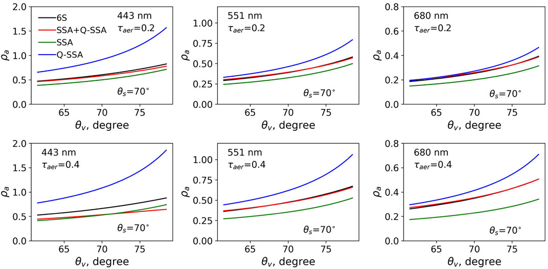
FIGURE 1. Atmospheric reflectance
Once the reflectance of the cloud/surface layer,
Analytical formulas developed by Zege et al. (1991) for optically thick scattering layers in the non-absorbing medium are used for
Next, the daily mean PAR,
where
In the final step, the individual daily mean estimates obtained on the source grid (number varies from 1 to 13 depending on geographical location, the time during the year, and data availability) are first remapped to an 18.4 km equal-area grid and weight-averaged using the cosine of the Sun zenith angle and then remapped to a Plate Carrée (equal-angle) grid with 18.4 km resolution at the equator. The remapping algorithm is exactly the one used by NASA OBPG to generate a Level 3 binned ocean color products (https://oceancolor.gsfc.bnasa/gov/docs/format/l3bins). Triangular-based linear interpolation is used to fill missing pixels at the edges.
The weighting procedure to obtain the final
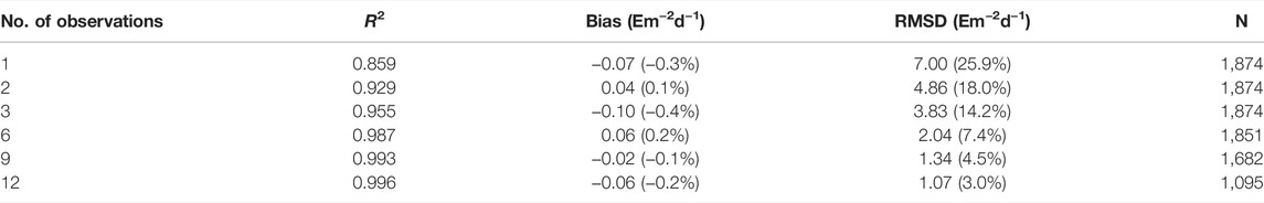
TABLE 1. Statistics of comparing
A way to reduce the sampling biases in such situations, not yet implemented in the algorithm, is to use MERRA-2 hourly cloud products for the very day of the EPIC observations, as proposed by Tan et al. (2020). If
where
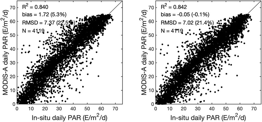
FIGURE 2. MODIS-A <
Associating uncertainty to each
The procedure described in Frouin et al. (2018a, b) is used to estimate and provide, for each pixel of the daily mean PAR product, the algorithm uncertainty component of the total uncertainty budget, which is expected to dominate. The bias and standard deviation portions are calculated as a function of clear sky daily mean PAR,
Figure 3 displays the resulting uncertainty (bias and standard deviation) on individual <EPAR> estimates as a function of
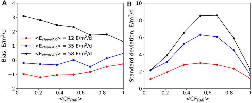
FIGURE 3. Algorithm uncertainity on individual <
As mentioned above, a complete per-pixel uncertainty budget must include errors in the Level 1b data, which may require estimating the sensitivity of
The EPIC <EPAR> product has been evaluated against in situ measurements at three mid-latitude oceanic sites (Figure 4), where long-term
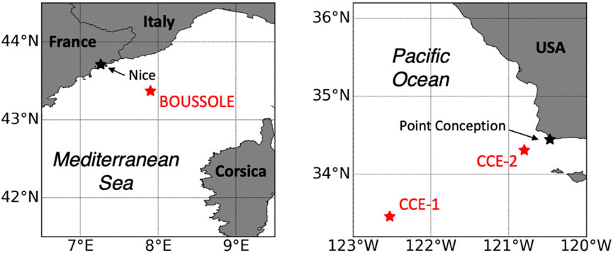
FIGURE 4. Location of the three in situ sites (BOUSSOLE in the Western Mediterranean Sea and CCE-1 and -2 in the Northeast Pacific Ocean) used to evaluate EPIC <
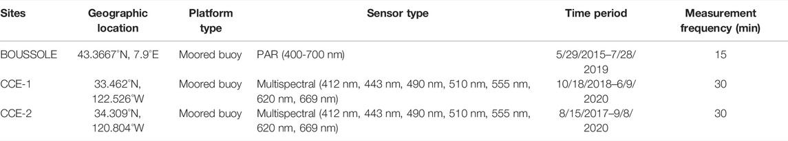
TABLE 2. I Characteristics of the in situ above surface downward solar irradiance datasets used in the evaluation of the EPIC
The BOUSSOLE above-surface downward solar irradiance dataset (http://www.obs-vlfr.fr/Boussole/html/project/boussole.php; Antoine et al., 2008) consists of high frequency
The CCE-1 and -2 datasets were collected at two surface moorings in the California Current (http://mooring.ucsd.edu/cce/). Multiple deployments are available and for this study we used the CCE-1 deployments from October 23, 2017 to June 9, 2020, and the CCE-2 deployments from August 15, 2017 to May 7, 2019. CCE-1 is located at 33.46°N, 122.53°W in the core of California Current, approximately 220 km off Point Conception, California. The CCE-2 mooring is operated at 34.31°N and 120.80°W and closer to the shore, approximately 35 km off Point Conception. For both mooring locations, the
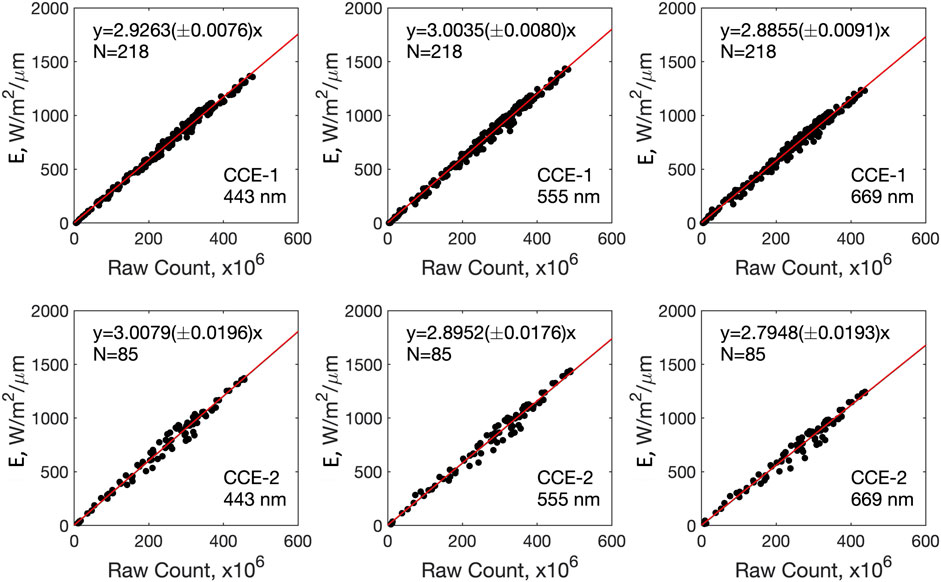
FIGURE 5. Examples of derived calibration coefficients for CCE-1 (deployment #13) and CCE-2 (deployment #9) datasets at 443, 559, and 669 nm. Raw counts are compared with E simulation in conditions of clear sky with small aerosol optical thickness (see text for details).
The calibrated datasets need to be checked and eventual biases removed before evaluating the EPIC
The BOUSSOLE dataset, however, was checked against 6S simulations. The same procedure as described for CCE-1 and -2 datasets, including the selection of clear sky days with small aerosol content and
Figure 6 displays scatter plots of 6S-simulated versus measured
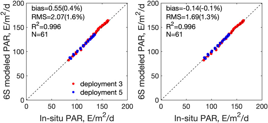
FIGURE 6. Comparison between 6S-modeled and field-measured instantaneous <
EPIC
Figure 7 displays for each site scatter plots of EPIC, MODIS-Aqua, and MODIS-Terra PAR estimates versus in situ measurements. In the comparisons, MODIS values at 9.2 km resolution were averaged to the 18.4 km resolution. The satellite estimates agree with the measurements, but statistical performance is better using EPIC, with bias and RMSD of 0.12 Em−2d−1 (0.4%) and 3.93 Em−2d−1 (12.0%) for BOUSSOLE, -0.5 Em−2d−1 (−1.5%) and 3.4 Em−2d−1 (10.2%) for CCE-1, and 0.8 Em−2d−1 (2.2%) and 4.6 Em−2d−1 (13.3%) for CCE-2. The MODIS-Aqua and -Terra estimates are more biased and exhibit more scatter, reflecting the points made above about using one instead of multiple observations during the day. In particular, the positive bias obtained with MODIS data is likely due to a higher probability of having clear skies at the time of satellite overpass, i.e., late morning or early afternoon, yielding higher than actual daily mean values. Such overestimation was documented in many studies (Section 1) and recently reported by Tan et al. (2020), who compared Medium Resolution Imaging Spectrometer (MERIS)
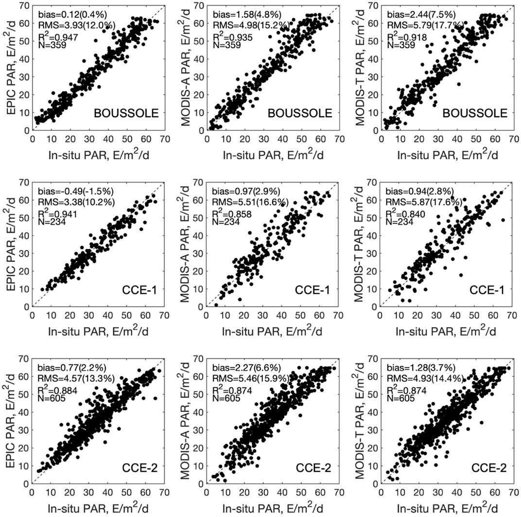
FIGURE 7. Comparison of EPIC, MODIS-T, <
Algorithm uncertainty was calculated for each
Figures 8A–C displays an example of an EPIC
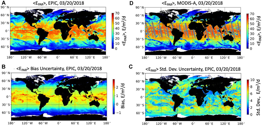
FIGURE 8. (A) <
Compared with the MODIS-Aqua
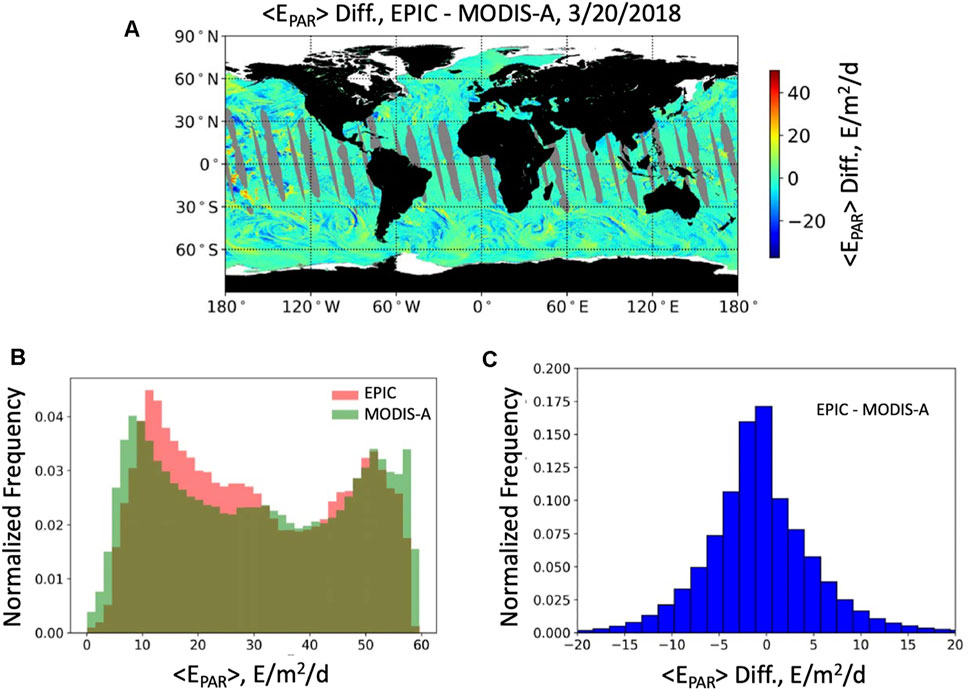
FIGURE 9. (A) Map of the difference between EPIC and MODIS-A <
The EPIC
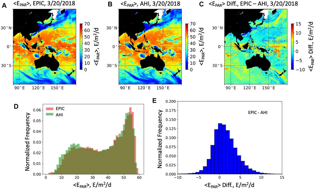
FIGURE 10. (A) <
Figure 11 displays the time series of EPIC and MODIS daily and monthly mean
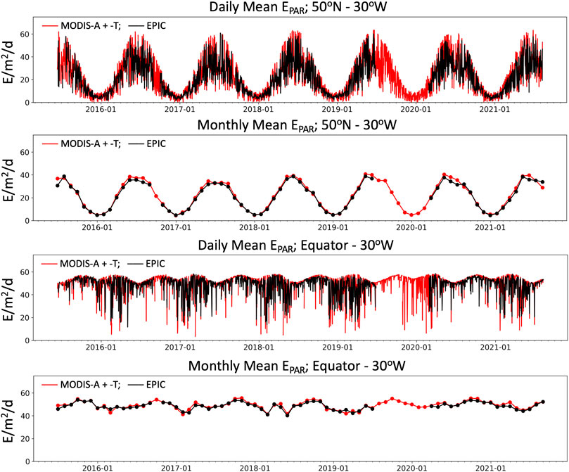
FIGURE 11. Time series of EPIC and MODIS-A and -T daily and monthly mean
An algorithm was developed to estimate daily mean PAR at the ice-free ocean surface,
The EPIC
The current algorithm can be improved in several ways, i.e., by calculating atmospheric reflectance more accurately at large zenith angles (LUTs may be used instead of approximate analytical representation), by relaxing the Lambertian assumption in the retrieval of the cloud/surface layer reflectance, by improving the parameterization of cloud bidirectional effects, and by including from reanalysis data information about cloud variability, which would provide better accuracy when only a few EPIC observations are available to estimate the daily means. Uncertainty may also be specified as a function of angular geometry and latitude, even region, instead of using an average estimate for all latitudes over several years of MERRA-2 data, and they can be fitted by a generalized additive model with proper auxiliary variables.
Other
The EPIC
The methodology can be easily extended to estimating ultraviolet (UV) surface irradiance using the EPIC spectral bands centered on 317, 325, 340, and 388 nm, especially since ozone content, a key variable governing atmospheric transmittance in the UV, is a standard EPIC product. Furthermore, planar and scalar fluxes below the surface, as well as average cosine for total light (a measure of the angular structure of the light field), variables more directly relevant to addressing science questions pertaining to biogeochemical cycling of carbon, nutrients, and oxygen can also be estimated without major difficulty from the above-surface quantities. Approaches have been identified and procedures devised (Frouin et al., 2018a); they are based on LUTs of clear sky and overcast situations and the derived cloud factor,
The raw data supporting the conclusion of this article will be made available by the authors, without undue reservation.
All the authors participated in the conception and organization of the study, the interpretation of the results, and the writing of the findings. RF and JT arranged the contents of the sections and wrote the first version of the manuscript. RF developed the algorithm to estimate ocean surface PAR. MC and DR created LUTs to associate uncertainties. JT coded the algorithms and performed the statistical analyses. MS implemented the processing line at the NASA Center for Climate Simulation and organized data archival at the Atmospheric Science Data Center. HM provided information about the AHI PAR product. DA, US, JS, and VV were involved in the field data collection and processing at the mooring sites. Everyone critically revised the manuscript.
The work effort to accomplish the study was funded by the National Aeronautics and Space Administration (NASA) under DSCOVR Grant 80NSSC19K0764 (Program Manager: R. S. Eckman) and by the Japan Aerospace Exploration Agency (JAXA) under GCOM-C Contract JX-PSPC-515384. The CCE moorings are funded by National Oceanic and Atmospheric Administration (NOAA) GOMO and OAP under Grant OAR4320278 Award# 304593. The BOUSSOLE data used in this work were collected when the project was funded by the European Space Agency, the Centre National d’Etudes Spatiales (CNES) and JAXA.
Authors DR and MC are employed by HYGEOS. The remaining authors declare that the research was conducted in the absence of any commercial or financial relationships that could be construed as a potential conflict of interest.
All claims expressed in this article are solely those of the authors and do not necessarily represent those of their affiliated organizations, or those of the publisher, the editors, and the reviewers. Any product that may be evaluated in this article, or claim that may be made by its manufacturer, is not guaranteed or endorsed by the publisher.
The authors gratefully acknowledge the various teams that produced and quality-controlled the EPIC data used in the study, the NASA OBPG for generating and making available the MODIS and VIIRS products, and JAXA for providing the AHI imagery via the P-Trees System. They also thank everyone involved in servicing the field instruments and collecting, processing, and archiving the BOUSSOLE, CCE-1 and CCE-2, and COVE solar irradiance data, and the MERRA-2 Science Team for the reanalysis data. The CCE-1 and CCE-2 moorings are part of the global OceanSITES program.
Antoine, D., André, J.-M., and Morel, A. (1996). Oceanic Primary Production: 2. Estimation at Global Scale from Satellite (Coastal Zone Color Scanner) Chlorophyll. Glob. Biogeochem. Cycles 10, 57–69. doi:10.1029/95GB02832
Antoine, D., Guevel, P., Desté, J.-F., Bécu, G., Louis, F., Scott, A. J., et al. (2008). The "BOUSSOLE" Buoy-A New Transparent-To-Swell Taut Mooring Dedicated to Marine Optics: Design, Tests, and Performance at Sea. J. Atmos. Ocean. Technol. 25, 968–989. doi:10.1175/2007jtecho563.1
Baker, K. S., and Frouin, R. (1987). Relation between Photosynthetically Available Radiation and Total Insolation at the Ocean Surface under clear Skies1. Limnol. Oceanogr. 32, 1370–1377. doi:10.4319/lo.1987.32.6.1370
Ballabrera-Poy, J., Murtugudde, R., Zhang, R.-H., and Busalacchi, A. J. (2007). Coupled Ocean-Atmosphere Response to Seasonal Modulation of Ocean Color: Impact on Interannual Climate Simulations in the Tropical Pacific. Am. Meteorol. Soc. 20, 353–374. doi:10.1175/JCLI3958.1
Behrenfeld, M. J., Boss, E., Siegel, D. A., and Shea, D. M. (2005). Carbon-based Ocean Productivity and Phytoplankton Physiology from Space. Glob. Biogeochem. Cycles 19, GB1006. doi:10.1029/2004GB002299
Behrenfeld, M. J., and Falkowski, P. G. (1997). Photosynthetic Rates Derived from Satellite-Based Chlorophyll Concentration. Limnol. Oceanogr. 42, 1–20. doi:10.4319/lo.1997.42.1.0001
Behrenfeld, M. J., O’Malley, R. T., Siegel, D. A., McClain, C. R., Sarmiento, J. L., Feldman, G. C., et al. (2006). Climate-driven Trends in Contemporary Ocean Productivity. Nature 444, 752–755. doi:10.1038/nature05317
Behrenfeld, M. J., Randerson, J. T., McClain, C. R., Feldman, G. C., Los, S. O., Tucker, C. J., et al. (2001). Biospheric Primary Production during an ENSO Transition. Science 291, 2594–2597. doi:10.1126/science.1055071
Bergman, J. W., and Salby, M. L. (1996). Diurnal Variations of Cloud Cover and Their Relationship to Climatological Conditions. J. Clim. 9, 2802–2820. doi:10.1175/1520-0442(1996)009<2802:dvocca>2.0.co;2
Carr, M.-E., Friedrichs, M. A. M., Schmeltz, M., Noguchi Aita, M., Antoine, D., Arrigo, K. R., et al. (2006). A Comparison of Global Estimates of marine Primary Production from Ocean Color. Deep Sea Res. Part Topical Stud. Oceanography 53, 741–770. doi:10.1016/j.dsr2.2006.01.028
Cox, C., and Munk, W. (1954). Measurement of the Roughness of the Sea Surface from Photographs of the Sun's Glitter. J. Opt. Soc. Am. 44, 838–850. doi:10.1364/JOSA.44.000838
Curran, P. J., and Dungan, J. L. (1989). Estimation of Signal-To-Noise: a New Procedure Applied to AVIRIS Data. IEEE Trans. Geosci. Remote Sensing 27, 620–628. doi:10.1109/tgrs.1989.35945
Dedieu, G., Deschamps, P. Y., and Kerr, Y. H. (1987). Satellite Estimation of Solar Irradiance at the Surface of the Earth and of Surface Albedo Using a Physical Model Applied to Metcosat Data. J. Clim. Appl. Meteorol. 26, 79–87. doi:10.1175/1520-0450(1987)026<0079:seosia>2.0.co;2
Deschamps, P.-Y., Herman, M., and Tanré, D. (1983). Modélisation du rayonnement réfléchi par l’atmosphère et la terre entre 0.35 and 4 µm. France: ESA contract report 4393/8C/F/DO(SC)University of Lille, 155
Dubuisson, P., Labonnote, L.-C., Riedi, J., Compiègne, M., and Winiarek, V. (2016). “ARTDECO: Atmopsheric Radiative Transfer Data Base for Earth and Climate Observation,” in Proc. International Radiation Symposium (Auckland, New Zealand, 16–22. April 2016.
Fitzpatrick, M. F., Brandt, R. E., and Warren, S. G. (2004). Transmission of Solar Radiation by Clouds over Snow and Ice Surfaces: A Parameterization in Terms of Optical Depth, Solar Zenith Angle, and Surface Albedo. J. Clim. 17, 266–275. doi:10.1175/1520-0442(2004)017<0266:tosrbc>2.0.co;2
IOCCG (2019). Uncertainties in Ocean Colour Remote Sensing. Editor F. Mélin (Dartmouth, Canada: IOCCG Report Series, No. 18, International Ocean Colour Coordinating Group). doi:10.25607/OBP-696
Frouin, R., and Chertock, B. (1992). A Technique for Global Monitoring of Net Solar Irradiance at the Ocean Surface. Part I: Model. J. Appl. Meteorol. 31, 1056–1066. doi:10.1175/1520-0450(1992)031<1056:atfgmo>2.0.co;2
Frouin, R., Franz, B. A., and Werdell, P. J. (2003). “The SeaWiFS PAR Product,” in Algorithm Updates for the Fourth SeaWiFS Data Reprocessing, NASA Tech. Memo. 2003-206892,. Editors S. B. Hooker, and E. R. Firestone (Greenbelt, Maryland: NASA Goddard Space Flight Center), Vol. 22, 46–50.
Frouin, R., and Iacobellis, S. F. (2002). Influence of Phytoplankton on the Global Radiation Budget. J. Geophys. Res. 107, 5–10. doi:10.1029/2001JD000562
Frouin, R., Ramon, D., Jolivet, D., and Compiègne, M. (2018b). Specifying Algorithm Uncertainties in Satellite-Derived PAR Products. Proc. SPIE 8525, 107780W. doi:10.1117/12.2501681
Frouin, R., and McPherson, J. (2012). Estimating Photosynthetically Available Radiation at the Ocean Surface from GOCI Data. Ocean Sci. J. 47, 313–321. doi:10.1007/s12601-012-0030-6
Frouin, R., McPherson, J., Ueyoshi, K., and Franz, B. A. (2012). A Time Series of Photosynthetically Available Radiation at the Ocean Surface from SeaWiFS and MODIS Data. Remote Sensing Mar. Environ., 19–12. doi:10.1117/12.981264
Frouin, R., and Murakami, H. (2007). Estimating Photosynthetically Available Radiation at the Ocean Surface from ADEOS-II Global Imager Data. J. Oceanogr. 63, 493–503. doi:10.1007/s10872-007-0044-3
Frouin, R., and Pinker, R. T. (1995). Estimating Photosynthetically Active Radiation (PAR) at the Earth's Surface from Satellite Observations. Remote Sensing Environ. 51, 98–107. doi:10.1016/0034-4257(94)00068-x
Frouin, R., Ramon, D., Boss, E., Jolivet, D., Compiègne, M., Tan, J., et al. (2018a). Satellite Radiation Products for Ocean Biology and Biogeochemistry: Needs, State-Of-The-Art, Gaps, Development Priorities, and Opportunities. Front. Mar. Sci. 5 10778, 3. doi:10.3389/fmars.2018.00003
Gelaro, R., McCarty, W., Suárez, M. J., Todling, R., Molod, A., Takacs, L., et al. (2017). The Modern-Era Retrospective Analysis for Research and Applications, Version 2 (MERRA-2). J. Clim. 30, 5419–5454. doi:10.1175/jcli-d-16-0758.1
Henson, S. A., Sarmiento, J. L., Dunne, J. P., Bopp, L., Lima, I., Doney, S. C., et al. (2010). Detection of Anthropogenic Climate Change in Satellite Records of Ocean Chlorophyll and Productivity. Biogeosciences 7, 621–640. doi:10.5194/bg-7-621-2010
Herman, J., HuangMcPeters, L. R., McPeters, R., Ziemke, J., Cede, A., and Blank, K. (2018). Synoptic Ozone, Cloud Reflectivity, and Erythemal Irradiance from Sunrise to sunset for the Whole Earth as Viewed by the DSCOVR Spacecraft from the Earth-Sun Lagrange 1 Orbit. Atmos. Meas. Tech. 11, 177–194. doi:10.5194/amt-11-177-2018
JGCM-100 (2008). Evaluation of Measurement Data—Guide to the Expression of Uncertainty in Measurement, Document Produced by Working Group 1 of the Joint Committee for Guides in Metrology (Jcgm/Wg 1), Published by the JCGM Member Organizations, 134. Sèvres: BIPM, IEC, IFCC, ILAC, ISO, IUPAC, IUPAP and OIML.
Jin, Z., Charlock, T. P., Smith, W. L., and Rutledge, K. (2004). A Parameterization of Ocean Surface Albedo. Geophys. Res. Lett. 31. 1180.doi:10.1029/2004GL021180
Kahru, M., Kudela, R., Manzano-SarabiaSarabia, M., and Mitchell, B. G. (2009). Trends in Primary Production in the California Current Detected with Satellite Data. J. Geophys. Res. 114, C02004. doi:10.1029/2008JC004979
Kim, J., Yang, H., Choi, J.-K., Moon, J.-E., and Frouin, R. (2016). Estimating Photosynthetically Available Radiation from Geostationary Ocean Color Imager (GOCI) Data. Korean J. Remote Sensing 32, 253–262. doi:10.7780/kjrs.2016.32.3.5
Kirk, J. T. O. (1994). Light and Photosynthesis in Aquatic Ecosystems. Bristol: Cambridge University Press.
Kotchenova, S. Y., Vermote, E. F., and Frouin, E. F. (2007). Validation of a Vector Version of the 6S Radiative Transfer Code for Atmospheric Correction of Satellite Data. Part II: Homogeneous Lambertian and Anisotropic Surfaces. Appl. Opt. 46, 4455. doi:10.1364/ao.46.004455,
Kotchenova, S. Y., Vermote, E. F., Matarrese, R., and Klemm, (2006). Validation of a Vector Version of the 6S Radiative Transfer Code for Atmospheric Correction of Satellite Data. Part I: Path Radiance. Appl. Opt. 45, 6762. doi:10.1364/ao.45.006762
Laliberté, J., Bélanger, S., and Frouin, R. (2016). Evaluation of Satellite-Based Algorithms to Estimate Photosynthetically Available Radiation (PAR) Reaching the Ocean Surface at High Northern Latitudes. Remote Sensing Environ. 184, 199–211. doi:10.1016/j.rse.2016.06.014
Lee, Y. J., Matrai, P. A., Friedrichs, M. A. M., Saba, V. S., Antoine, D., Ardyna, M., et al. (2015). An Assessment of Phytoplankton Primary Productivity in the Arctic Ocean from Satellite Ocean Color/In Situ Chlorophyll‐ a Based Models. J. Geophys. Res. Oceans 120, 6508–6541. doi:10.1002/2015JC011018
Loeb, N. G., Wielicki, B. A., Su, W., Loukachine, K., Sun, W., Wong, T., et al. (2007). Multi-instrument Comparison of Top-Of-Atmosphere Reflected Solar Radiation. Am. Meteorol. Soc. 20, 575–591. doi:10.1175/JCLI4018.1
Longhurst, A., Sathyendranath, S., Platt, T., and Caverhill, C. (1995). An Estimate of Global Primary Production in the Ocean from Satellite Radiometer Data. J. Plankton Res. 17, 1245–1271. doi:10.1093/plankt/17.6.1245
Marshak, A., Herman, J., Adam, S., Karin, B., Carn, S., Cede, A., et al. (2018). Earth Observations from DSCOVR EPIC Instrument. Bull. Amer. Meteorol. Soc. 99, 1829–1850. doi:10.1175/BAMS-D-17-0223.1
Miller, A. J., Alexander, M. A., Boer, G. J., Chai, F., Denman, K., Erickson, D. J., et al. (2003). Potential Feedbacks between Pacific Ocean Ecosystems and Interdecadal Climate Variations. Bull. Amer. Meteorol. Soc. 84, 617–634. doi:10.1175/BAMS-84-5-617
Mobley, C. D., and Boss, E. S. (2012). Improved Irradiances for Use in Ocean Heating, Primary Production, and Photo-Oxidation Calculations. Appl. Opt. 51, 6549–6560. doi:10.1364/AO.51.006549
Murtugudde, R., Beauchamp, J., McClain, C. R., Lewis, M., and Busalacchi, A. J. (2002). Effect of Penetrative Radiation on the Upper Tropical Ocean Circulation. J. Clim. 15, 470486. doi:10.1175/1520-0442(2002)015<0470:eoprot>2.0.co;2
Nakamoto, S., Kumar, S. P., Oberhuber, J. M., Ishizaka, J., Muneyama, K., and Frouin, R. (2001). Response of the Equatorial Pacific to Chlorophyll Pigment in a Mixed Layer Isopycnal Ocean General Circulation Model. Geophys. Res. Lett. 28, 2021–2024. doi:10.1029/2000GL012494
Nakamoto, S., Kumar, S. P., Oberhuber, J. M., Muneyama, K., and Frouin, R. (2000). Chlorophyll Modulation of Sea Surface Temperature in the Arabian Sea in a Mixed-Layer Isopycnal General Circulation Model. Geophys. Res. Lett. 27, 747–750. doi:10.1029/1999GL002371
Platt, T., Denman, K. L., and Jassby, A. D. (1977). “Modeling the Productivity of Phytoplankton,” in The Sea: Ideas and Observations on Progress in the Study of the Seas. Editor E. D. Goldberg (New York, NY: John Wiley, 807–856.
Platt, T., Forget, M.-H., White, G. N., Caverhill, C., Bouman, H., Devred, E., et al. (2008). Operational Estimation of Primary Production at Large Geographical Scales. Remote Sensing Environ. 112, 3437–3448. doi:10.1016/j.rse.2007.11.018
Povey, A. C., and Grainger, R. G. (2015). Known and Unknown Unknowns: Uncertainty Estimation in Satellite Remote Sensing. Atmos. Meas. Tech. 8, 4699–4718. doi:10.5194/amt-8-4699-2015
Ramon, D., Jolivet, D., Tan, J., and Frouin, R. (2016). “Estimating Photosynthetically Available Radiation at the Ocean Surface for Primary Production (3P Project): Modeling, Evaluation, and Application to Global MERIS Imagery,” in Proc. SPIE 9878” in Remote Sensing of the Oceans and Inland Waters: Techniques, Applications, and Challenges, 98780D. doi:10.1117/12.2229892
Rossow, W. B., and Schiffer, R. A. (1999). Advances in Understanding Clouds from ISCCP. Bull. Amer. Meteorol. Soc. 80, 2261–2287. doi:10.1175/1520-0477(1999)080<2261:aiucfi>2.0.co;2
Ryther, J. H. (1956). Photosynthesis in the Ocean as a Function of Light Intensity1. Limnol. Oceanogr. 1, 61–70. doi:10.4319/lo.1956.1.1.0061
Shell, K. M., Frouin, R., Nakamoto, S., and Somerville, R. C. J. (2003). Atmospheric Response to Solar Radiation Absorbed by Phytoplankton. J. Geophys. Res. 108, 4445. doi:10.1029/2003JD003440
Somayajula, S. A., Devred, E., Bélanger, S., Antoine, D., Vellucci, V., and Babin, M. (2018). Evaluation of Sea-Surface Photosynthetically Available Radiation Algorithms under Various Sky Conditions and Solar Elevations. Appl. Opt. 57, 3088–3105. doi:10.1364/ao.57.003088
Sweeney, C., Gnanadesikan, A., Griffies, S. M., Harrison, M. J., Rosati, A. J., and Samuels, B. L. (2005). Impacts of Shortwave Penetration Depth on Large-Scale Ocean Circulation and Heat Transport. J. Phys. Oceanogr. 35, 1103–1119. doi:10.1175/jpo2740.1
Tan, J., and Frouin, R. (2019). Seasonal and Interannual Variability of Satellite‐Derived Photosynthetically Available Radiation over the Tropical Oceans. J. Geophys. Res. Oceans 124, 3073–3088. doi:10.1029/2019JC014942
Tan, J., FrouinJolivet, R. D., Jolivet, D., Compiègne, M., and Ramon, D. (2020). Evaluation of the NASA OBPG MERIS Ocean Surface PAR Product in clear Sky Conditions. Opt. Express 28, 33157. doi:10.1364/OE.3960610.1364/oe.396066
Tan, S.-C., and Shi, G.-Y. (2012). The Relationship between Satellite-Derived Primary Production and Vertical Mixing and Atmospheric Inputs in the Yellow Sea Cold Water Mass. Continental Shelf Res. 48, 138–145. doi:10.1016/j.csr.2012.07.015
Tanré, D., Herman, M., Deschamps, P. Y., and De Leffe, A. (1979). Atmospheric Modeling for Space Measurements of Ground Reflectances, Including Bidirectional Properties. Appl. Opt. 18, 3587–3594. doi:10.1364/ao.18.003587
Uitz, J., Claustre, H., Gentili, B., and Stramski, D. (2010). Phytoplankton Class-specific Primary Production in the World's Oceans: Seasonal and Interannual Variability from Satellite Observations. Glob. Biogeochem. Cycles 24, a–n. doi:10.1029/2009GB003680
Wald, L. (1989). Some Examples of the Use of Structure Functions in the Analysis of Satellite Images of the Ocean. Photogramm. Eng. Rem. Sen. 55, 1487–1490.
Wang, Y., and Zhao, C. (2017). Can MODIS Cloud Fraction Fully Represent the Diurnal and Seasonal Variations at DOE ARM SGP and Manus Sites? J. Geophys. Res. Atmos. 122, 329–343. doi:10.1002/2016JD025954
Yang, Y., Zhao, C., and Fan, H. (2020). Spatiotemporal Distributions of Cloud Properties over China Based on Himawari-8 Advanced Himawari Imager Data. Atmos. Res. 240, 104927. doi:10.1016/j.atmosres.2020.104927
Zege, E. P., Ivanov, A. P., and Katsev, I. L. (1991). Image Transfer through a Scattering Medium. New York: Springer-Verlag, 349.
Keywords: photosynthetically available radiation, satellite remote sensing, Lagrange L1 orbit, EPIC sensor, DSCOVR mission, light absorption and scattering, ocean biogeochemistry
Citation: Frouin R, Tan J, Compiègne M, Ramon D, Sutton M, Murakami H, Antoine D, Send U, Sevadjian J and Vellucci V (2022) The NASA EPIC/DSCOVR Ocean PAR Product. Front. Remote Sens. 3:833340. doi: 10.3389/frsen.2022.833340
Received: 11 December 2021; Accepted: 02 March 2022;
Published: 12 April 2022.
Edited by:
Gregory Schuster, National Aeronautics and Space Administration (NASA), United StatesReviewed by:
Chuanfeng Zhao, Beijing Normal University, ChinaCopyright © 2022 Frouin, Tan, Compiègne, Ramon, Sutton, Murakami, Antoine, Send, Sevadjian and Vellucci. This is an open-access article distributed under the terms of the Creative Commons Attribution License (CC BY). The use, distribution or reproduction in other forums is permitted, provided the original author(s) and the copyright owner(s) are credited and that the original publication in this journal is cited, in accordance with accepted academic practice. No use, distribution or reproduction is permitted which does not comply with these terms.
*Correspondence: Robert Frouin, cmZyb3VpbkB1Y3NkLmVkdQ==
Disclaimer: All claims expressed in this article are solely those of the authors and do not necessarily represent those of their affiliated organizations, or those of the publisher, the editors and the reviewers. Any product that may be evaluated in this article or claim that may be made by its manufacturer is not guaranteed or endorsed by the publisher.
Research integrity at Frontiers
Learn more about the work of our research integrity team to safeguard the quality of each article we publish.