Cloud Height Daytime Variability From DSCOVR/EPIC and GOES-R/ABI Observations

One of the largest uncertainties in climate sensitivity predictions is the influence of clouds. While some aspects of cloud formation and evolution are well understood, others such as the diurnal variability of their heights remains largely unexplored at global scales. Aiming to fill that fundamental gap in cloud knowledge, this paper studies the daytime evolution of cloud top height using the EPIC instrument aboard the DSCOVR satellite, complemented by coincident cloud height retrievals by GOES-R’s ABI instrument. Both datasets indicate that cloud height exhibits a minimum around midday for low clouds with amplitudes between 250 and 600 m depending on the season. The two datasets also agree that high clouds exhibit a contrasting behavior with steady increase of cloud height from morning to evening. We investigate dependences on the type of underlying surface, finding that the amplitude of the diurnal cycles is weaker over ocean than over land for both EPIC and ABI retrievals. We also find a positive correlation between cloud fraction and height over ocean which turns negative over land for low clouds, while for high clouds the correlation is largely positive.

Introduction

The diurnal variability of cloud fraction and its associated radiative influence is linked to the evolution of the boundary layer depth, determined by the balance between entrainment, subsidence, advection, and turbulent fluxes (Antonia et al., 1977; Wood and Bretherton 2004; Guo et al., 2011; Painemal et al., 2013; Mazzitelli et al., 2014). Solar heating drives air to rise, which then cools adiabatically until it reaches saturation with respect to liquid or ice, and forms droplets or ice particles. Over land, as the sun heats the surface, cloud cover starts increasing early in the morning as the boundary layer deepens, reaching a maximum around noon and early afternoon and continuing with a decrease of cloud cover later in the afternoon. Over ocean, cloud cover evolution follows a diametrically opposite cycle: peak cloud fraction during nighttime, followed by decrease during the morning, a minimum around noon, and a steady increase during the afternoon (Delgado-Bonal et al., 2020a; Delgado-Bonal et al., 2021).

Besides cloud fraction, cloud height is the other main cloud property greatly affecting the Earth’s greenhouse effect, and its response to increasing surface temperature represents a strong but not well-understood feedback process in the climate system (Zelinka and Hartmann (2010); Davies and Molloy 2012). Knowledge of cloud top and cloud base help to reduce the estimation of uncertainties of cloud forcing (Xu et al., 2021). Long-term trends in global cloud heights have not been quantified yet, partially due to large interannual fluctuations associated with major regional events such as ENSO that mask low frequency variability.

Although the signal of cloud height changes on a global scale may not be clear, changes in the regional level are detectable because the amplitude of at those scales can be much larger than the changes in the globally-averaged value. Analyses with the Multiangle Imaging SpectroRadiometer (MISR) instrument on the Terra satellite found unexplained differences between the Northern and Southern Hemisphere from March 2000 to February 2015, the former decreasing the cloud top height averaged value at −16 ± 5 m/decade and the latter increasing it at 14 ± 4 m/decade (Davies and Molloy 2012; Evan and Norris 2012; Davies et al., 2017).

At smaller temporal and spatial scales, fluctuations of cloud height are even more dramatic. Interannual global variations of cloud top heights reveal significant signals, with anomalies up to 80 m due to La Niña [2007–2008 and 2011] and El Niño [2009, 2013] events. Metrics of ENSO and Hadley-Walker circulations strength also correlate significantly with the interannual regional changes in cloud height (Davies et al., 2017).

Cloud height variability has been observed with a variety of sensors applying different principles to retrieve cloud top height (Marchand 2013; Lelli et al., 2014). Zhao et al. (2020) used MODIS data from 2000 to 2018 to conclude that cloud top height in East Asia has increased at an average rate of 0.020 km per year, exhibiting different seasonal rates and a positive correlation with sea surface temperature, indicating that cloud top height may be modulated by changes close to the surface (Zhao et al., 2020). Using reflected solar ultraviolet-visible (UV-VIS) measurements taken from 1996 to 2003 by the global ozone monitoring experiment (GOME) instrument, Loyola et al. (2010) obtained a decreasing cloud top height trend of −4.8 m per year within the ±60° of latitude belt.

The drastic changes of cloud height inter-annual variations at different scales give an idea of the importance of analyzing regional features. Small land areas such as in the Zhao et al. (2020) study over East Asia find different sign and order of magnitude for cloud height changes compared to the entire Northern Hemisphere (Davies et al., 2017). Additionally, the magnitudes of the changes differ between land and ocean and are ultimately driven by the climatology of each region.

Higher frequency cloud height changes such as diurnal variations are difficult to analyze globally given the orbital characteristics of sun-synchronous satellites. For example, while the MISR instrument aboard the Terra satellite could be used to study interannual variations (Davies and Molloy 2012), its fixed equator crossing time at approximately 10:30 am local time does not allow it to quantify diurnal variations in cloud height. The importance of monitoring cloud diurnal variabilities cannot be overstated since they are intimately related to the planet’s energy balance and climate change. Even with other cloud properties remaining unchanged, changes in the diurnal variability of cloud fraction of various cloud types could have an important impact on the net radiation at surface (Cairns 1995). As an example, early deforestation in the Amazon basin led to a change of low and high cloud fractions, resulting in a change of local cloud diurnal contribution to the time-mean shortwave surface flux of 20 Wm^-2, equivalent to a change of 0.05 in surface albedo (Cutrim et al., 1995).

As the boundary layer depth changes every day, a repeating cycle of cloud cover and cloud height manifests itself. Variability in the height of low clouds has been reported for different regions, mainly stratocumulus regions in the southeastern Pacific (Minnis and Harrison 1984; Minnis et al., 1992; Zuidema et al., 2009) where modulations of the boundary layer are attributed to the blocking effects of the Andes which increases subsidence and induces convergence and upward motions in the lower troposphere (Painemal et al., 2013; Zuidema et al., 2009). In situ observations in this region have also documented the diurnal pattern of cloud height (de Szoeke et al., 2012) and although limited in their sampling frequency, suggest that cloud top heights exhibit diurnal variations in this region that are larger than in the northeast Pacific (Minnis et al., 1992; Garreaud et al., 2001; Bretherton et al., 2010), highlighting once again the importance of regional features and topography on the diurnal cycles of cloud top height.

Diurnal changes in cloud height have also been studied with numerical models (Garreaud et al., 2001). Unfortunately, it is well-known that these models have poor skill in simulating realistically the diurnal evolution of cloud properties, which materializes as underestimation of amplitudes and misplacement of the local times of maximum and minimum cloud top height occurrence (Abel et al., 2010; Yin and Porporato 2017).

Quantifying global diurnal variations in cloud height requires resolving simultaneously and with high accuracy both temporal and spatial gradients. On the spatial side, techniques with high vertical resolution such as radio occultation fail to provide spatial information (von Engeln et al., 2005), while active instruments despite offering excellent vertical resolution suffer from limited horizontal coverage, as in the case of Cloud–Aerosol Lidar and Infrared Pathfinder Satellite Observations (CALIPSO). On the temporal side, sampling limitations that come with sun-synchronous orbits (Zuidema et al., 2009; Xie et al., 2012) affect instruments such as the Moderate Resolution Imaging Spectroradiometer (MODIS) and MISR.

Extensive spatial coverage is crucial for understanding the regional nuances in cloud diurnal cycles. Geostationary satellite systems such as GOES-R (currently including GOES-16 and GOES-17) combine extensive spatial coverage with a high-frequency sampling of 10 min. These satellites rely on visible and infrared measurements to track cloud coverage and vertical motions. The infrared bands of the Advanced Baseline Imager (ABI) are used to simultaneously retrieve Cloud Top Height, Cloud Top Temperature, and Cloud Top Pressure for each cloudy pixel (Schmit et al., 2017). Earlier satellites of the GOES family have been used to quantify the diurnal cycles of marine clouds in the southeastern Pacific (Minnis et al., 1992; Painemal et al., 2013).

However, to obtain a truly global and detailed view of planetary cloudiness beyond what is provided by a single geostationary satellite, it is necessary to either aggregate data from multiple geostationary and sun-synchronous satellites as is done by the International Satellite Cloud Climatology Project (ISCCP) (Rossow and Schiffer, 1991) or to use the recently available measurements of the Earth Polychromatic Imaging Camera (EPIC) aboard the Deep Space Climate Observatory (DSCOVR) spacecraft (Marshak et al., 2018). EPIC observes the planet from approximately 1.5 million km, always facing the sunlit side of the planet. Unlike the GOES-R satellites which relies on thermal infrared bands, EPIC derives the cloud height from observations of the O2 A-band (779.5 and 764 nm), and B-band (680 and 688 nm) pairs (Yang et al., 2019).

In this study, we use retrievals from both EPIC and ABI aboard GOES-R to quantify the diurnal evolution of cloud top height for their overlapping coverage area. Previous analyses of cloud fraction from EPIC and ISCCP showed that the diurnal evolution of high and low cloud fractions is different (Cairns 1995; Delgado-Bonal et al., 2021), However, the accompanying cycles of cloud top heights have hitherto not been examined. Here, we apply a separation between high and low clouds to resolve more meaningfully the diurnal cycle of height for different kinds of clouds.

Data and Methods Section presents a brief overview of the ABI and EPIC cloud effective height algorithms, and details the methodology used to study diurnal variations of cloud height. Absolute values of cloud height depend critically on the technique and wavelengths used in the derivation and cannot generally be directly compared. However, we maintain that it is acceptable to compare relative changes in cloud top height between different measurement techniques and between measurements and models (Davies et al., 2017). Quantifying the amplitude and shape of diurnal cloud height cycles derived from two sensors using different retrieval principles can serve as a two-way cross-validation of the respective retrievals. Results Section describes in some detail the cloud height cycles of low and high clouds from EPIC and ABI, both from global and regional perspective. EPIC and ABI are alike from the perspective of being able to track regional cloudiness throughout the daytime, albeit at a smaller spatial scale for ABI. To provide a statistically reliable picture of the cloud height diurnal cycles, we aggregate observations at hourly local times. Once the diurnal evolution of cloud coverage and height has been fully described in terms of cloud fraction and height, we evaluate the correlation between the two variables throughout their daily global evolution. This paper employs the EPIC statistically derived diurnal maps at fixed local times to investigate the correlation of cloud fraction and cloud top height in order to characterize regional behavior.

Data and Methods

The NOAA product from the GOES-R series of satellites provides an official binary clear-sky mask, classifying each pixel as clear or cloudy. The cloud mask algorithm uses 9 out of the 16 ABI spectral bands to detect clouds based on spectral, spatial and temporal signatures (Heidinger, 2012). The thresholds for this binary classification were derived from analysis of space-borne lidar and current geostationary imager data. The primary validation sources are data from Spinning Enhanced Visible and InfraRed Imager (SEVIRI) and the Cloud-Aerosol LIdar with Orthogonal Polarization (CALIOP) aboard the Cloud-Aerosol Lidar and Infrared Pathfinder Satellite Observations (CALIPSO) satellite. The latter has an inherent high sensitivity to cloud presence over all surface types and under all illumination conditions (Schmit et al., 2017).

GOES-R ABI infrared observations aiming to measure the height of clouds are impacted by their wavelength-dependent emissivity, and by emissions from the surface and atmosphere. Also, clouds often exhibit complex vertical structures that violate the assumptions of the single layer plane parallel models. To provide reliable cloud top retrievals, the ABI Cloud Height Algorithm (ACHA) uses the 13.3 µm CO₂ channels coupled with multiple longwave IR windows (10.4, 11 and 12 µm) within an optimal estimation framework where an analytical radiative transfer model has central role. Cloud-top pressure and cloud-top height are derived from the cloud-top temperature product and the atmospheric temperature profile provided by Numerical Weather Prediction data. GOES-R retrievals combine therefore the sensitivity to cloud height offered by the CO₂ channel with the sensitivity to ice cloud microphysics offered by the window channels, so no microphysical assumptions need to be invoked (Heidinger and Straka 2013).

EPIC’s 2,048 × 2,048 pixel CCD array provides reflectances at ten channels spanning from the ultraviolet (318, 325, 340, and 388 nm) to the visible (443, 551, 680, and 688 nm) and near infrared (764 and 780 nm). The cloud product algorithm uses a surface-type based threshold method for cloud masking, applied on the reflectances at the 388, 680, 780 nm and O2 A- and B-band channels. The results are comparable with those provided by geostationary (GEO) and low Earth orbit (LEO) satellites, with differences of only 1.5% in the global cloud fraction of collocated datasets (Yang et al., 2019). The EPIC cloud mask algorithm provides confidence level flags for its cloud detection outcomes; less than 3% of the total number of pixels are flagged as low confidence cloudy.

Unlike ABI, the EPIC cloud top height is derived from observations of O₂ A-band (779.5 and 764 nm) and B-band (680 and 688 nm) pairs. Due to photon penetration into the cloud, for a given optical thickness and particle properties, the radiance measured by EPIC’s A- and B-bands is not only a function of cloud top height, but also a function of the cloud extinction coefficient profile (Yang et al., 2013). Therefore, EPIC’s retrievals correspond to an “effective” cloud top height, a measure of the mean height from which light is scattered (“centroid”), an important parameter that has been widely used in trace gas retrievals and climate studies (Stammes et al., 2008; Wang et al., 2011; Joiner et al., 2012). Since ABI-derived cloud top heights from IR methods are also not true geometrical top heights, and therefore also considered “effective,” but in a different sense, we will simply refer to “cloud top height” in many of the discussions that follow, with the understanding that the retrieval principles for the two cases are very different and responsible for the discrepancies in cloud top height values.

The EPIC A-band and B-band cloud effective pressure retrievals are based on the Mixed Lambertian-Equivalent Reflectivity concept, extensively studied and applied in operational settings (Koelemeijer et al., 2001; Wang et al., 2008; Joiner et al., 2012; Yang et al., 2013). In this model, it is assumed that the pixel contains two Lambertian reflectors, the surface and the cloud. The cloud is assumed to be opaque, i.e., no photon penetration occurs (even if that is not true in reality). Cloud effective pressure and cloud effective fraction are simultaneously retrieved and converted to cloud height using the co-located atmosphere profile provided by GEOS-5 FP-IT (Lucchesi, 2015). EPIC cloud effective height can be obtained either from the A- or B-band, providing slightly different values due to the difference in photon penetration depths, which contains information on cloud vertical structure. In this paper, we use the less noisy A-band value (Yang et al., 2019).

Both EPIC and GOES-R products are labeled in UTC time. Exploiting their vast coverage areas, each dataset can be split into different local time zones depending on the longitude and UTC acquisition time. Figure 1 shows an EPIC RGB image whose clouds have been enhanced for the purpose of illustration. The center of the image always corresponds to local noon, while the left and right edges to sunrise and sunset respectively. Since EPIC acquires up to 13 (in Boreal winter) and up to 22 (in Boreal summer) images per day, the local time of observation for various regions varies by day, providing thus an average diurnal cycle of cloudiness when accumulated over time. Geostationary satellites with their high frequency data acquisition are also capable of observing cloud evolution throughout the day, but their coverage is limited to a fixed portion of the Earth. In order to create comparable datasets for EPIC and GOES-R, we partition the observation field into 1 × 1 grid cells. We follow a nearest neighbor algorithm to find the matching grid cell for each pixel by minimizing the Euclidean distance between the longitude and latitude coordinates of each pixel and the center of each grid cell. We then calculate average values of cloud height for each grid cell.

FIGURE 1

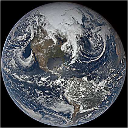
FIGURE 1. EPIC RGB image corresponding to 2020-05-01 17:54:31 UTC. The image has been enhanced to show the cloud coverage in detail.

By making use of the ability to track the daily evolution of cloud properties, we split the data into local hourly bins, creating 24 local time maps for each satellite’s imagery. For EPIC, we repeat this process with 4 years of data from June 2015 to June 2019 (approximately 16,500 full disk images) while for ABI we use all the available retrievals for 2020 (approximately 52,500 images). The DSCOVR satellite was placed in a safe mode in June 2019 for almost 9 months, prompting us to use the 4 years of consistent data prior to that date. For the purposes of our statistics, we assume an ergodic seasonal behavior which allows us to average each season of data for the 4 years to obtain a single mean map for each season. For ABI, we use the latest complete full year available and average by season. Given the large amount of data captured by ABI, 1 year of data is sufficient to provide stable statistics. We then average the cloud height of all the local time maps across the number of observations for each grid cell and across all years for a particular season, obtaining thus seasonally-averaged maps of cloud height at all local times.

This methodology has proven useful in determining diurnal cycles with EPIC data and quantifying the diurnal variability of cloud fraction for low and high clouds consistently with previous research (Delgado-Bonal et al., 2021). Due to EPIC’s location at the L1 point, the best pixel resolution is achieved at nadir ( ∼ 8 km); off nadir the pixels become elliptical with the long axis larger by a factor of about 1/cos(SZA) and the short axis unaffected. Furthermore, as the Earth’s axis is tilted 23.5° relative to its orbital plane around the Sun, high northern latitudes in boreal winter and high southern latitudes in boreal summer are excluded from EPIC’s field of view. Moreover, some regions suffer discontinuity behaviors in contiguous zones along meridians during December-January-February due to lower availability of data at specific local times, but broad patterns can be easily inferred by observing adjacent zones.

We quickly realized that the diurnal behavior of high and low clouds is distinct and thus study it separately. We consider all ABI clouds below 3,000 m as low clouds, and all clouds above 6,000 m as high clouds. Changing these cutoffs by ±1,000 m does not impact our results substantially. For EPIC, we assign the low and high cloud classes based on the most likely thermodynamic cloud phase (liquid or ice) provided in the Level 2 datasets (Yang et al., 2019) with all liquid clouds classified as low and all ice clouds classified as high. EPIC’s cloud thermodynamic phase determination is based on cloud effective temperature, which is inferred from the cloud effective pressure derived from the EPIC O₂ A-band observations (Meyer et al., 2016; Yang et al., 2019). Cloudy pixels are classified as ice if the effective temperature is lower than 240K, and as liquid if it exceeds 260K, while the rest of cloudy pixels are classified as unknown to avoid potentially erroneous classifications. This methodology has been tested against MODIS (Meyer et al., 2016), yielding agreement in the thermodynamic phase of approximately 77% of the pixels, categorizing 21% of them as unknown, and misclassifying only about 2% with respect to MODIS. By using the most likely thermodynamic phase, we avoid possible distortions of the daytime cycles due to misclassified pixels.

Results

Integrated Area Results

While diurnal variations in cloud top height have been previously reported for regions of various sizes, ranging from specific locations of field experiments to larger domains spanning like Eastern Asia or the contiguous United States, there has never been a truly global analysis. In this section, EPIC is employed for this task. At the same time, we also examine the degree to which EPIC’s views of cloud top height diurnal patterns are consistent with those from ABI over land (GOES-16) and over ocean (GOES-17). Similar to the low/high discrimination, land-ocean separation is important for capturing the distinct nature of continental and marine clouds, expected to have different amplitudes and phases in their diurnal cycles. A prerequisite for such an analysis is matching the overlapping portions of domains viewed by EPIC and ABI.

To avoid potential sunrise and sunset artifacts at the edge of EPIC images, we only consider pixels with local times between early morning (8:00) and late afternoon (16:00), while for ABI we extend to nighttime. Figure 2 shows the diurnal cycle results for the integrated area of GOES-16 over land, along with the same area for EPIC, and the full global average of EPIC. Each column represents one season, with the top panels corresponding to high clouds and the bottom panel to low clouds.

FIGURE 2

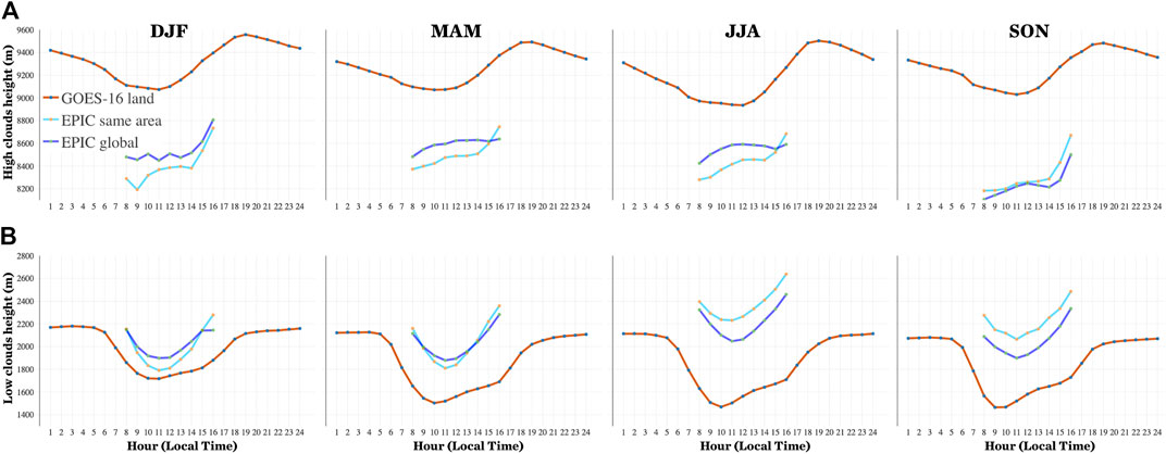
FIGURE 2. Diurnal cycles of cloud height for GOES-16 (red line) and EPIC over land. EPIC results are shown for the whole globe (dark blue) and for the same areas as GOES-16 (light blue). Each column is a different season for high (A) and low (B) clouds.

ABI cloud top height diurnal cycles for low clouds over land reveal a minimum around 10 am Local Time (LT), whose amplitude varies from approximately 250 m in boreal winter to a maximum of 600 m in boreal summer. The same area analyzed with EPIC yields a minimum around 11 am LT and an amplitude of approximately 450 m. The cycles for the whole globe obtained with EPIC have similar shape as that for the GOES-16 domain although slightly displaced in the vertical axis.

Along with the mean values, we determine the standard deviation of the mean for each 1-by-1 degree cell. Then, we average the standard deviation for the whole globe to provide an hourly global standard deviation associated with every hourly point showed in Figures 2, 3. For low clouds over land, we obtain a standard deviation of approximately 550 m for ABI, and of 500 m for EPIC. This value of standard deviation indicates that the effective cloud top heights even within the same cloud group (low/high) exhibit significant variability for a particular time of the day. For example, in our analysis, clouds at 7,000 m and at 14,000 m are considered high clouds and are aggregated together in our statistical analyses. To obtain the sampling error of the mean, we divide the standard deviation by the square root of the size of sample and multiply the result with the Z score of a 95% confidence interval (Z = 1.96). By doing so, we obtain a sampling error of less than 10 m for both EPIC and ABI. This suggests that our sample is sufficiently large to calculate mean values accurately.

FIGURE 3

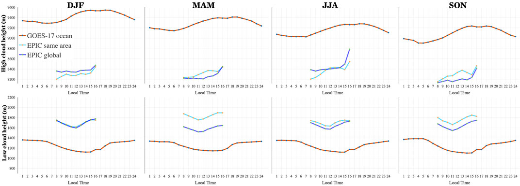
FIGURE 3. As Figure 2, but for GOES-17 over ocean.

As stated above, direct comparison of the absolute values of cloud top heights derived from instruments with different capabilities and algorithmic philosophies is not advisable. Furthermore, differences arise since low clouds for GOES-R have been defined as those with tops below 3,000 m whereas EPIC uses a definition directly linked to retrieved thermodynamic phase. We therefore focus only on comparing the shapes of the diurnal cycle curves. Despite the different definitions, the existence of a characteristic diurnal cycle of cloud height even at these very large scales is undeniable in both cases, echoing behavior previously seen only in regional studies (Zuidema et al., 2009; An et al., 2017; Painemal et al., 2013; Zhao et al., 2020).

The cycles of high clouds over land show a distinctive sinusoidal wave shape. For GOES-16, cloud top height has a minimum before noon followed by a steady increase that peaks around 19 h. Throughout the day, the standard deviation for high clouds is approximately 600 m. For the same area, EPIC generally shows the same monotonic increase during the day, with a maximum at the time of the last retrieval we retain, at 4 pm LT, with a standard deviation around 500 m. In this case, global results deviate from the regional picture: although an increase in cloud top effective height during daytime is seen, it is not as clear as that for the GOES-17 disc.

Figure 3 shows the corresponding results for GOES-17 and EPIC, this time over ocean. The marine environment has a discriminating effect on the amplitude of the cycles, which is manifested in both low and high clouds. GOES-17 results for low clouds indicate that the magnitude of the diurnal cycle is approximately 200 m, which matches the EPIC results for the same region and for the whole globe, as well as previous findings in the southern Pacific (Painemal et al., 2013). The cycles for high clouds are also characterized by smaller amplitudes, with their minima shifted to early morning for GOES-17 but maintaining the same progressive increase during daytime for both satellites. The standard deviation for both EPIC and GOES-R is approximately 500 m for clouds over ocean.

Diurnal Cycle Maps

Figure 4 shows two distinct moments of the diurnal low cloud height cycles in boreal spring for GOES-16 (top) and GOES-17 (bottom). The left column presents the average cloud top height between 11:00 am and noon LT, while the right column shows the same disc at midnight. The figures illustrate the transition over land from lower clouds around noon (blue hues) to higher clouds at midnight (red hues). A smaller total change from noon to midnight is seen over ocean. The land grid cells of the two GOES-16 colormaps of Figure 4, when averaged, provide two of the points for the timeseries of Figure 2. Similarly, two of the points of Figure 3 come from the average of ocean only grid cells for the GOES-17 images in Figure 4.

FIGURE 4

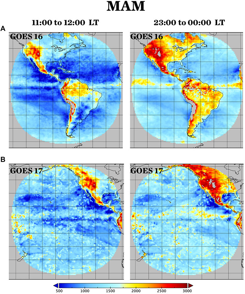
FIGURE 4. GOES-16 (A) and GOES-17 (B) diurnal cycle of low clouds height in meters. Left column shows the cloud top height at noon local time and the right column shows the values at midnight. Cloud top height is higher during nighttime for both satellites.

The diurnal cycles for low clouds seen by EPIC have the same broad characteristics. Since EPIC observations are limited to daytime, Figure 5 shows the global view of cloud top height at early morning, noon and evening. The morning-to-noon transition is characterized by a shift from red to blue shades, only to be followed by an increase of cloud top height in the afternoon, recovering the distinctive red tints over most of the continental areas. While these cycles are generally similar across the globe, regional differences can be spotted by careful examination of Figure 5. For example, by looking at the diurnal cycles over the United States and Brazil, one observes that Brazil shows the expected increase in the afternoon while half of the United States area remains with lower cloud heights. Besides being regionally dependent, the diurnal cycles evolve throughout the year.

FIGURE 5

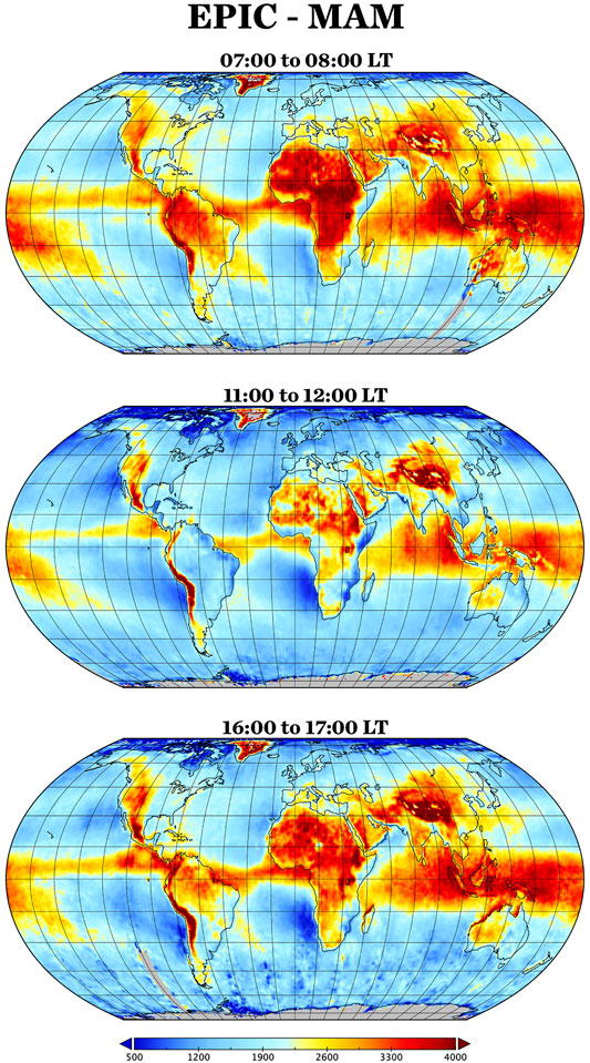
FIGURE 5. EPIC cloud height for liquid clouds in meters at three selected times for Boreal spring.

Cloud Fraction/Cloud Height Correlation

Previous analyses studying the potential link between cloud fraction and cloud height have been limited to the correlation in time derived from daily data. For example, Gryspeerdt et al. (2014) investigated the strength of the relationships between cloud fraction and cloud top pressure (which translates to cloud top height) using data from MODIS Terra, defining the correlation as the slope of a linear regression between the two quantities. The study found a strong interrelationship between the two variables, likely due to deep convective systems having both high cloud fraction and cloud height. However, given Terra’s fixed equator crossing time at 10:30 am, these findings do not inform us about intraday correlations.

Once the diurnal cycles of cloud fraction (Delgado-Bonal et al., 2021) and cloud height have been characterized using EPIC, their co-evolution during the day can be examined. In general, cloud fraction over land peaks around noon, which contrasts with the minimum cloud fraction over ocean found at that time. Due to this contrasting diurnal evolution of cloud fraction between land and ocean, An et al., 2017 found a negative correlation between cloud base height and cloud fraction over the contiguous United States, while Painemal et al., 2013 found a positive correlation between cloud top height and cloud fraction for two locations over the southern Pacific. However, the sign of these correlations is not necessarily representative of ocean and land behavior overall, as evidenced by the variety of diurnal behaviors seen regionally. Figure 6 shows two examples of oceanic regions, only 5° in latitude apart, with opposing correlations between cloud fraction and cloud effective height.

FIGURE 6

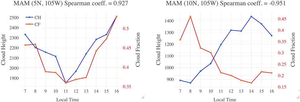
FIGURE 6. Example of diurnal evolution of cloud fraction and cloud effective height in meters using EPIC for two locations in the Pacific Ocean during Boreal spring. Even though the locations are physically close, they have opposite correlation coefficient sign.

To quantify correlation, we use Spearman’s ρ as a nonparametric measure of rank correlation (Myers and Well 2003, pp. 508) with a range between +1 (positive correlation) and −1 (negative correlation). This statistical quantity is not limited to linear correlations and assesses how well the relationship between two variables can be described using a monotonic function. A positive value of the coefficient indicates that as the value of one variable increases, so does the value of the other variable, and vice-versa. Figure 6 left shows an example of a positive correlation between cloud top height and cloud fraction seen by EPIC with a Spearman’s coefficient of +0.927 while the right side of the figure has a negative coefficient of −0.951.

Exploiting EPICs spatial and temporal advantages, Figure 7 shows the correlation between cloud top height and cloud fraction for low clouds, separately for the four seasons. Over ocean, Boreal summer emerges as the season of strongest correlation, and with positive correlations dominating because as cloud fractions decrease during daytime over ocean, reaching a minimum around noon, cloud top heights also decrease, a state of affairs also reported by Painemal et al., 2013. However, it must be noted that this is not a general finding since other oceanic locations such as the west coast of central America are characterized by a negative correlation during boreal summer that turns positive during boreal winter. The variety of behaviors highlights the importance of EPIC in characterizing diurnal cycles.

FIGURE 7

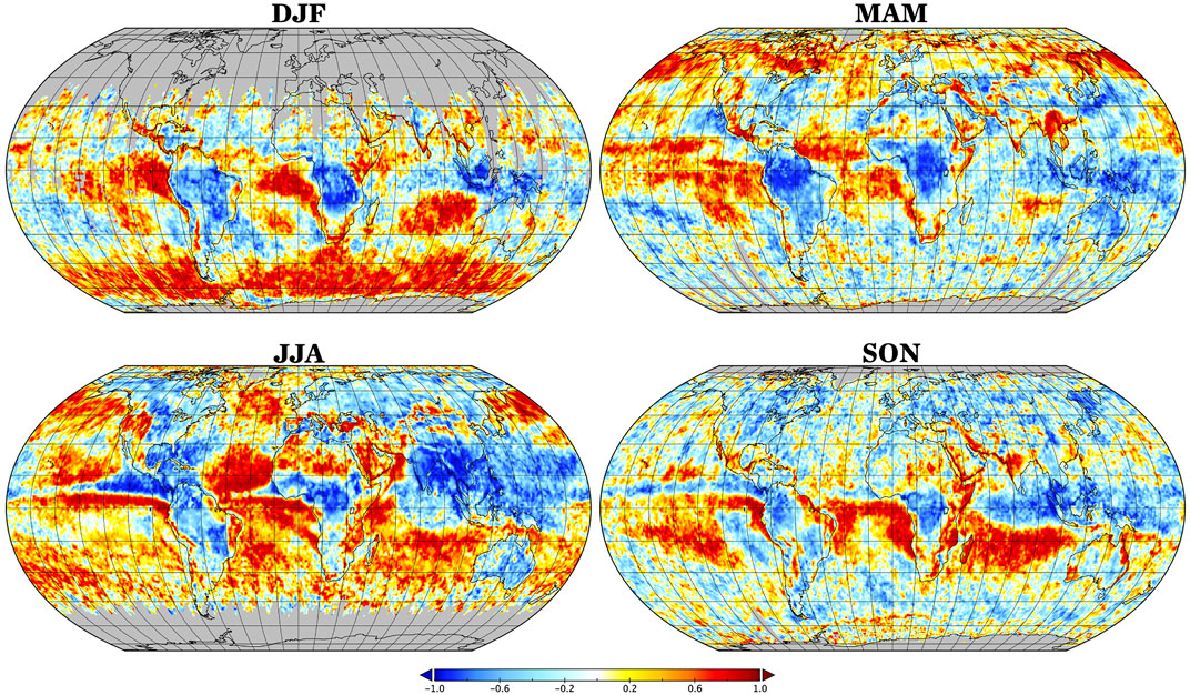
FIGURE 7. Spearman correlation coefficient between cloud fraction and cloud effective height for low clouds using EPIC. Blue colors indicate a negative correlation while red colors a positive one.

Figure 8 shows EPIC’s counterpart correlation map for high clouds. In this case, a positive correlation between high cloud fraction and cloud height is observed for most of the globe. High cloud fraction evolves diurnally regardless of the surface type, with higher cloud fraction values in the afternoon than in the morning and noon (see discussion and appendixes in Delgado-Bonal et al., 2021). The diurnal cloud height cycles obtained in this paper (see Figures 2, 3) follow a similar behavior during the day, with cloud height increasing from morning to evening, hence resulting in mostly positive regional correlations.

FIGURE 8

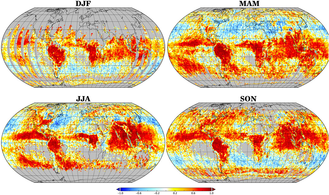
FIGURE 8. As Figure 7 but for high clouds.

Conclusions and Discussion

Radiation fluxes depend strongly and nonlinearly on the diurnal variations of cloud properties (Bergman and Salby 1997; Delgado-Bonal et al., 2020b), with the amount of radiation reflected to space depending on how cloud fraction changes during daytime correlate with the cycle of solar insolation. On the thermal infrared side, cloud height is also a major controlling factor of the planet’s energy balance since low and high clouds have different impacts on the greenhouse effect. Understanding cloud height variability is thus essential for the characterization of the planet’s climate. While previous research has focused on interannual variability or regional studies because of lack of appropriate observations, this paper employs appropriate data from EPIC and GOES-R to study diurnal cloud top height cycles over large areas.

EPIC and ABI use different principles and parts of the spectrum to retrieve cloud top height, so the physical meaning of what cloud height they retrieve and how it relates to the true geometrical cloud top height is different. We use this to our advantage to show that, regardless of methodology, the diurnal cycles of cloud height for both low and high clouds cannot only be clearly inferred, but also compared in terms of their relative shapes which have a prominent signal for even global averages. Sensible changes in thresholds or definitions used to distinguish between low and high clouds do not impact the conclusions in any meaningful way.

To provide a holistic view of daytime cloud height cycles for the entire planet EPIC retrievals are more appropriate. The results from this instrument are generally in agreement with those from the ABI instrument aboard geostationary satellites, and prior research which was more geographically limited. EPIC theoretical analyses show that its cloud height retrievals are influenced by the solar zenith angle (SZA); because of the observation geometry from the L1 point is essentially the same as the viewing zenith angle, a convex shape with a minimum during midday was expected (Yang et al., 2013). The extent of the impact of such a systematic dependence is unknown. In order to minimize possible interference of a geometrical artifact in the results, we elected to report the diurnal cycles only from 8 am to 4 pm LT. EPIC results for the integrated areas presented in Figures 2, 3 did indeed reveal the expected convex behavior for low clouds. At the same time, our results show that: 1) we can achieve consistency with previous findings; 2) the convex behavior is not found for high clouds; 3) the amplitudes of those convex cycles are different between land and ocean; and 4) the diurnal cycles from ABI are similar even though these retrievals are not affected by the same geometrical effects.

Finally, we explore the daytime correlation between cloud fraction and cloud height Since the thermodynamic and dynamical structure of the location may affect that relationship, we develop global correlation maps using Spearman’s coefficient. We show that, for low clouds, the correlation is seasonally and regionally dependent, being generally positive over ocean and negative over land as a consequence of the opposite diurnal behavior of cloud fraction for the two underlying surfaces. On the other hand, high clouds are positively correlated for the most part of the globe since the amounts of high clouds evolve independently of the surface type.

In summary, we showed that:

• For low clouds, cloud height exhibits a minimum around midday with amplitudes between 250 and 600 m. On the contrary, high clouds exhibit a steady increase from morning to evening of approximately 500 m.

• The amplitude of the diurnal cycles is smaller over ocean than over land.

• The correlation between cloud fraction and height for low clouds is mostly positive over ocean and negative over land. For high clouds, the correlation is largely positive.

Data Availability Statement

The data sets used in this investigation are available at the NASA’s Atmospheric Science Data Center (ASDC), located in the Science Directorate located at NASA'S Langley Research Center in Hampton, Virginia. The collection is called “DSCOVR EPIC CLOUD Product Version 03” and is accessible at: https://earthdata.nasa.gov/eosdis/daacs/asdc. EPIC images are accessible at: https://epic.gsfc.nasa.gov.

Author Contributions

AD-B and AM. analyzed the data. YY developed the EPIC L2 cloud datasets. AD-B, AM, YY, and LO discussed the results and wrote the paper.

Funding

AD-B research was supported by the DSCOVR Science Management project. AM acknowledges support from NASA's DSCOVR Science Management project. YY would like to acknowledge funding support from the NASA DSCOVR Science Team Program. LO gratefully acknowledges support from NASA’s MEaSUREs program.

Conflict of Interest

The authors declare that the research was conducted in the absence of any commercial or financial relationships that could be construed as a potential conflict of interest.

Publisher’s Note

All claims expressed in this article are solely those of the authors and do not necessarily represent those of their affiliated organizations, or those of the publisher, the editors and the reviewers. Any product that may be evaluated in this article, orclaim that may be made by its manufacturer, is not guaranteed or endorsed by the publisher.

References

Abel, S. J., Walters, D. N., and Allen, G. (2010). Evaluation of Stratocumulus Cloud Prediction in the Met Office Forecast Model during VOCALS-REx. Atmos. Chem. Phys. 10, 10541–10559. doi:10.5194/acp-10-10541-2010

CrossRef Full Text | Google Scholar

An, N., Wang, K., Zhou, C., and Pinker, R. T. (2017). Observed Variability of Cloud Frequency and Cloud-Base Height within 3600 M above the Surface over the Contiguous United States. J. Clim. 30 (10), 3725–3742. doi:10.1175/JCLI-D-16-0559.1

CrossRef Full Text | Google Scholar

Antonia, R. A., Danh, H. Q., and Prabhu, A. (1977). Response of a Turbulent Boundary Layer to a Step Change in Surface Heat Flux. J. Fluid Mech. 80 (1), 153–177. doi:10.1017/S002211207700158X

CrossRef Full Text | Google Scholar

Bergman, J. W., and Salby, M. L. (1997). The Role of Cloud Diurnal Variations in the Time-Mean Energy Budget. J. Clim. 10, 1114–1124. doi:10.1175/1520-0442(1997)010<1114:trocdv>2.0.co;2

CrossRef Full Text | Google Scholar

Bretherton, C. S., Wood, R., George, R. C., Leon, D., Allen, G., and Zheng, X. (2010). Southeast Pacific Stratocumulus Clouds, Precipitation and Boundary Layer Structure Sampled along 20° S during VOCALS-REx. Atmos. Chem. Phys. 10, 10639–10654. doi:10.5194/acp-10-10639-2010

CrossRef Full Text | Google Scholar

Cairns, B. (1995). Diurnal Variations of Cloud from ISCCP Data. Atmos. Res. 37, 1–3. doi:10.1016/0169-8095(94)00074-N

CrossRef Full Text | Google Scholar

Cutrim, E., Martin, D. W., and Rabin, R. (1995). Enhancement of Cumulus Clouds over Deforested Lands in Amazonia. Bull. Amer. Meteorol. Soc. 76, 1801–1805. doi:10.1175/1520-0477(1995)076<1801:eoccod>2.0.co;2

CrossRef Full Text | Google Scholar

Davies, R., Jovanovic, V. M., and Moroney, C. M. (2017). Cloud Heights Measured by MISR from 2000 to 2015. J. Geophys. Res. Atmos. 122, 3975–3986. doi:10.1002/2017JD026456

CrossRef Full Text | Google Scholar

Davies, R., and Molloy, M. (2012). Global Cloud Height Fluctuations Measured by MISR on Terra from 2000 to 2010. Geophys. Res. Lett. 39, a–n. doi:10.1029/2011GL050506

CrossRef Full Text | Google Scholar

de Szoeke, S. P., Yuter, S., Mechem, D., Fairall, C. W., Burleyson, C. D., and Zuidema, P. (2012). Observations of Stratocumulus Clouds and Their Effect on the Eastern Pacific Surface Heat Budget along 20°S. J. Clim. 25 (24), 8542–8567. doi:10.1175/JCLI-D-11-00618.1

CrossRef Full Text | Google Scholar

Delgado-Bonal, A., Marshak, A., Yang, Y., and Holdaway, D. (2020b). Analyzing Changes in the Complexity of Climate in the Last Four Decades Using MERRA-2 Radiation Data. Sci. Rep. 10, 922. doi:10.1038/s41598-020-57917-8

PubMed Abstract | CrossRef Full Text | Google Scholar

Delgado-Bonal, A., Marshak, A., Yang, Y., and Oreopoulos, L. (2020a). Daytime Variability of Cloud Fraction from DSCOVR/EPIC Observations. J. Geophys. Res. Atmos. 125, e2019JD031488. doi:10.1029/2019JD031488

CrossRef Full Text | Google Scholar

Delgado-Bonal, A., Marshak, A., Yang, Y., and Oreopoulos, L. (2021). Global Daytime Variability of Clouds from DSCOVR/EPIC Observations. Geophys. Res. Lett. 48, e2020GL091511. doi:10.1029/2020GL091511

CrossRef Full Text | Google Scholar

Evan, A. T., and Norris, J. R. (2012). On Global Changes in Effective Cloud Height. Geophys. Res. Lett. 39, a–n. doi:10.1029/2012GL053171

CrossRef Full Text | Google Scholar

Garreaud, R. D., Rutllant, J., Quintana, J., Carrasco, J., and Minnis, P. (2001). CIMAR-5: A Snapshot of the Lower Troposphere over the Subtropical Southeast Pacific. Bull. Amer. Meteorol. Soc. 82 (10), 2193–2208. doi:10.1175/1520-0477-82.10.2193

CrossRef Full Text | Google Scholar

Gryspeerdt, E., Stier, P., and Grandey, B. S. (2014). Cloud Fraction Mediates the Aerosol Optical Depth-Cloud Top Height Relationship. Geophys. Res. Lett. 41, 3622–3627. doi:10.1002/2014GL059524

CrossRef Full Text | Google Scholar

Guo, J., Zhang, J., Yang, K., Liao, H., Zhang, S., Huang, K., et al. (2011). Investigation of Near-Global Daytime Boundary Layer Height Using High-Resolution Radiosondes: First Results and Comparison with ERA5, MERRA-2, JRA-55, and NCEP-2 Reanalyses. Atmos. Chem. Phys. 21, 17079–17097. doi:10.5194/acp-21-17079-2021

CrossRef Full Text | Google Scholar

Heidinger, A. (2012). ABI Cloud Height Algorithm Theoretical Basis Document. NOAA/NESDIS/STAR. Version 3.0 July.

Google Scholar

Heidinger, A., and Straka, W. C. (2013). ABI Cloud Mask Algorithm Theoretical Basis Document. NOAA/NESDIS/STAR, SSEC/CIMSS. Version 3.0 June 11.

Google Scholar

Joiner, J., Vasilkov, A. P., Gupta, P., Bhartia, P. K., Veefkind, P., Sneep, M., et al. (2012). Fast Simulators for Satellite Cloud Optical Centroid Pressure Retrievals; Evaluation of OMI Cloud Retrievals. Atmos. Meas. Tech. 5 (3), 529–545. doi:10.5194/amt-5-529-2012

CrossRef Full Text | Google Scholar

Koelemeijer, R. B. A., Stammes, P., Hovenier, J. W., and de Haan, J. F. (2001). A Fast Method for Retrieval of Cloud Parameters Using Oxygen A Band Measurements from the Global Ozone Monitoring Experiment. J. Geophys. Res. 106, 3475–3490. doi:10.1029/2000JD900657

CrossRef Full Text | Google Scholar

Lelli, L., Kokhanovsky, A. A., Rozanov, V. V., Vountas, M., and Burrows, J. P. (2014). Linear Trends in Cloud Top Height from Passive Observations in the Oxygen A-Band. Atmos. Chem. Phys. 14, 5679–5692. doi:10.5194/acp-14-5679-2014

CrossRef Full Text | Google Scholar

Loyola R., D. G., Thomas, W., Spurr, R., and Mayer, B. (2010). Global Patterns in Daytime Cloud Properties Derived from GOME Backscatter UV-VIS Measurements. Int. J. Remote Sensing 31 (16), 4295–4318. doi:10.1080/01431160903246741

CrossRef Full Text | Google Scholar

Lucchesi, R. (2015). File Specification for GEOS-5 FP-IT. GMAO Office Note No. 2 (Version1.3), 60. Available from http://gmao.gsfc.nasa.gov/pubs/office_notes.

Google Scholar

Marchand, R. (2013). Trends in ISCCP, MISR, and MODIS Cloud-Top-Height and Optical-Depth Histograms. J. Geophys. Res. Atmos. 118, 1941–1949. doi:10.1002/jgrd.50207

CrossRef Full Text | Google Scholar

Marshak, A., Herman, J., Adam, S., Karin, B., Carn, S., Cede, A., et al. (2018). Earth Observations from DSCOVR EPIC Instrument. Bull. Amer. Meteorol. Soc. 99, 1829–1850. doi:10.1175/BAMS-D-17-0223.1

PubMed Abstract | CrossRef Full Text | Google Scholar

Mazzitelli, I. M., Cassol, M., Miglietta, M. M., Rizza, U., Sempreviva, A. M., and Lanotte, A. S. (2014). The Role of Subsidence in a Weakly Unstable marine Boundary Layer: a Case Study. Nonlin. Process. Geophys. 21, 489–501. doi:10.5194/npg-21-489-2014

CrossRef Full Text | Google Scholar

Meyer, K., Yang, Y., and Platnick, S. (2016). Uncertainties in Cloud Phase and Optical Thickness Retrievals from the Earth Polychromatic Imaging Camera (EPIC). Atmos. Meas. Tech. 9, 1785–1797. doi:10.5194/amt-9-1785-2016

PubMed Abstract | CrossRef Full Text | Google Scholar

Minnis, P., and Harrison, E. F. (1984). Diurnal Variability of Regional Cloud and Clear-Sky Radiative Parameters Derived from GOES Data. Part II: November 1978 Cloud Distributions. J. Clim. Appl. Meteorol. 23 (7), 1012–1031. doi:10.1175/1520-0450(1984)023<1012:dvorca>2.0.co;2

CrossRef Full Text | Google Scholar

Minnis, P., Heck, P. W., Young, D. F., Fairall, C. W., and Snider, J. B. (1992). Stratocumulus Cloud Properties Derived from Simultaneous Satellite and Island-Based Instrumentation during FIRE. J. Appl. Meteorol. 31, 317–339. doi:10.1175/1520-0450(1992)031<0317:scpdfs>2.0.co;2

CrossRef Full Text | Google Scholar

Myers, J. L., and Well, A. D. (2003). Research Design and Statistical Analysis. 2nd ed. New York: Lawrence Erlbaum Associates Publishers.

Google Scholar

Painemal, D., Minnis, P., and O'Neill, L. (2013). The Diurnal Cycle of Cloud-Top Height and Cloud Cover over the Southeastern Pacific as Observed by GOES-10. J. Atmos. Sci. 70 (8), 2393–2408. doi:10.1175/JAS-D-12-0325.1

CrossRef Full Text | Google Scholar

Rossow, W. B., and Schiffer, R. A. (1991). ISCCP Cloud Data Products. Bull. Amer. Meteorol. Soc. 72, 2–20. doi:10.1175/1520-0477(1991)072<0002:icdp>2.0.co;2

CrossRef Full Text | Google Scholar

Schmit, T. J., Griffith, P., Gunshor, M. M., Daniels, J. M., Goodman, S. J., and Lebair, W. J. (2017). A Closer Look at the ABI on the GOES-R Series. Bull. Am. Meteorol. Soc. 98, 681–698. doi:10.1175/BAMS-D-15-00230.1

CrossRef Full Text | Google Scholar

Stammes, P., Sneep, M., de Haan, J. F., Veefkind, J. P., Wang, P., and Levelt, P. F. (2008). Effective Cloud Fractions from the Ozone Monitoring Instrument: Theoretical Framework and Validation. J. Geophys. Res. 113, D16S38. doi:10.1029/2007JD008820

CrossRef Full Text | Google Scholar

von Engeln, A., Teixeira, J., Wickert, J., and Buehler, S. A. (2005). Using CHAMP Radio Occultation Data to Determine the Top Altitude of the Planetary Boundary Layer. Geophys. Res. Lett. 32, L06815. doi:10.1029/2004GL022168

CrossRef Full Text | Google Scholar

Wang, P., Stammes, P., van der A, R., Pinardi, G., and van Roozendael, M. (2008). FRESCO+: an Improved O2 A-Band Cloud Retrieval Algorithm for Tropospheric Trace Gas Retrievals. Atmos. Chem. Phys. 8, 6565–6576. doi:10.5194/acp-8-6565-2008

CrossRef Full Text | Google Scholar

Wang, P., Stammes, P., and Mueller, R. (2011). Surface Solar Irradiance from SCIAMACHY Measurements: Algorithm and Validation. Atmos. Meas. Tech. 4, 875–891. doi:10.5194/amt-4-875-2011

CrossRef Full Text | Google Scholar

Wood, R., and Bretherton, C. S. (2004). Boundary Layer Depth, Entrainment, and Decoupling in the Cloud-Capped Subtropical and Tropical Marine Boundary Layer. J. Clim. 17 (18), 3576–3588. doi:10.1175/1520-0442(2004)017<3576:bldead>2.0.co;2

CrossRef Full Text | Google Scholar

Xie, F., Wu, D. L., Ao, C. O., Mannucci, A. J., and Kursinski, E. R. (2012). Advances and Limitations of Atmospheric Boundary Layer Observations with GPS Occultation over Southeast Pacific Ocean. Atmos. Chem. Phys. 12, 903–918. doi:10.5194/acp-12-903-2012

CrossRef Full Text | Google Scholar

Xu, H., Guo, J., Li, J., Liu, L., Chen, T., Guo, X., et al. (2021). The Significant Role of Radiosonde-Measured Cloud-Base Height in the Estimation of Cloud Radiative Forcing. Adv. Atmos. Sci. 38, 1552–1565. doi:10.1007/s00376-021-0431-5

CrossRef Full Text | Google Scholar

Yang, Y., Marshak, A., Mao, J., Lyapustin, A., and Herman, J. (2013). A Method of Retrieving Cloud Top Height and Cloud Geometrical Thickness with Oxygen A and B Bands for the Deep Space Climate Observatory (DSCOVR) Mission: Radiative Transfer Simulations. J. Quantitative Spectrosc. Radiative Transfer 122, 141–149. doi:10.1016/j.jqsrt.2012.09.017

CrossRef Full Text | Google Scholar

Yang, Y., Meyer, K., Wind, G., Zhou, Y., Marshak, A., Platnick, S., et al. (2019). Cloud Products from the Earth Polychromatic Imaging Camera (EPIC): Algorithms and Initial Evaluation. Atmos. Meas. Tech. 12, 2019–2031. doi:10.5194/amt-12-2019-2019

PubMed Abstract | CrossRef Full Text | Google Scholar

Yin, J., and Porporato, A. (2017). Diurnal Cloud Cycle Biases in Climate Models. Nat. Commun. 8, 2269. doi:10.1038/s41467-017-02369-4

PubMed Abstract | CrossRef Full Text | Google Scholar

Zelinka, M. D., and Hartmann, D. L. (2010). Why Is Longwave Cloud Feedback Positive? J. Geophys. Res. 115, D16117. doi:10.1029/2010JD013817

CrossRef Full Text | Google Scholar

Zhao, M., Zhang, H., Wang, H.-B., Zhou, X.-X., Zhu, L., An, Q., et al. (2020). The Change of Cloud Top Height over East Asia during 2000-2018. Adv. Clim. Change Res. 11 (2), 110–117. doi:10.1016/j.accre.2020.05.004

CrossRef Full Text | Google Scholar

Zuidema, P., Painemal, D., de Szoeke, S., and Fairall, C. (2009). Stratocumulus Cloud-Top Height Estimates and Their Climatic Implications. J. Clim. 22 (17), 4652–4666. doi:10.1175/2009JCLI2708.1

CrossRef Full Text | Google Scholar