- 1NASA-GSFC, Earth Sciences Division, Greenbelt, MD, United States
- 2GESTAR-II University of Maryland Baltimore County, Baltimore, MD, United States
- 3GESTAR-II Morgan State University, Baltimore, MD, United States
We update the parameterization capturing the variation of parameters that describe how cloud occurrence (layer cloud fraction) and layer cloud optical depth (COD) distributions overlap vertically. Our updated analysis is motivated by the availability of a new dataset constructed by combining two products describing the two-dimensional extinction properties of liquid and ice phase clouds (and their mixtures) according to active cloud observations by the CloudSat and CALIPSO satellites. As before, cloud occurrence overlap is modeled with the decorrelation length of an inverse exponential function describing the decay with separation distance of the relative likelihood that two cloudy layers are overlapped maximally versus randomly. Similarly, cloud optical depth distribution vertical overlap is described again with a decorrelation length that describes the assumed inverse exponential decay with separation distance of the rank correlation between cloud optical depth distribution members in two cloudy layers. We derive the climatological zonal variability of these two decorrelation lengths using 4 years of observations for scenes of ∼100 km scale length, a typical grid size of numerical models used for climate simulations. As previously, we find a strong latitudinal dependence reflecting systematic differences in dominant cloud types with latitude, but substantially different magnitudes of decorrelation length compared to the previous work. The previously used parameterization form is therefore updated with new parameters to describe the latitudinal dependence of decorrelation lengths and its seasonal shift. Similar zonal patterns of decorrelation length are found when the analysis is broken down by different cloud classes. When the revised parameterization is implemented in a cloud subcolumn generator, simulated column cloud properties compare to observations quite well, and so do their associated cloud radiative effects, but improvements over the earlier version of the parameterization are marginal.
1 Introduction
As long as climate and other Earth system models have grids that are large enough to compel the use of cloud schemes producing fractional cloudiness, i.e., as long as subgrid cloud variability exists implicitly without being explicitly resolved, the vertical overlap of cloud condensate has to be taken into account. This includes both the simple overlap of cloud occurrence at different vertical levels (aka “cloud fraction overlap,”) and also the overlap of the horizontal distribution of condensate amount. Assuming that cloud particle size is horizontally homogeneous (admittedly, a simplification) the latter overlap is practically equivalent to the overlap of cloud optical depth (COD) at different levels. Needless to say, that in the unrealistic case of no horizontal variability of condensate, i.e. horizontally homogeneous clouds, this type of overlap is no longer a concern.
Cloud fraction overlap and its impact on the transport of atmospheric radiation has been studied for many years. Prior to the 2000s the most prevalent description of cloud fraction overlap was the so-called “maximum-random” paradigm where contiguous cloud layers were assumed to overlap maximally, while non-contiguous layers (separated by cloudless layers) were assumed to overlap randomly. How exactly maximum-random overlap was perceived and conceptually implemented in practice varied widely. One variant due to Geleyn and Hollingsworth (1979) allowed for random overlap not only of cloudy layers separated by clear layers (non-contiguous cloud situations), but also of the parts of layers belonging to vertically contiguous cloud entities that extend beyond the coverage of a less cloudy intervening layer. Another variant assumes that all cloud layers within broad atmospheric layers, even when non-contiguous, form “blocks” where overlap is maximum, while these blocks overlap randomly (Chou et al., 1998). Regardless of the maximum-random overlap flavor, accounting for cloud fraction overlap in radiative transfer calculations is not trivial, especially in the shortwave part of the spectrum where a large fraction of the downwelling radiation is backscattered. This recognition motivated the introduction of the concept of “subcolumns.” Radiative calculations are manageable when the number of blocks is small: for example, when only three cloud blocks are allowed throughout the atmospheric column, only eight distinct permutations of cloudy subcolumns can exist (Chou et al., 1998). In the longwave part of the spectrum, as long as scattering is not explicitly resolved, any given conceptual implementation of maximum-random overlap allows the calculation of the fraction of upward and downward clear-line-of-sight for radiation propagation (Chou et al., 1999).
Our insight into cloud overlap changed greatly thanks to the seminal work of Hogan and Illingworth (2000) who used ground radar observations to show that the overlap of the area occupied by two cloud layers should not be viewed as the binary outcome of either maximum or random overlap, but rather as a continuum between the two possibilities that depends on the separation distance of the two layers (a more formal description will be presented in the next section). Not too long after (Räisänen et al., 2004; Pincus et al., 2005), the realization that cloudy layers are not horizontally homogeneous underscored the need for a description of how parts of a cloud layer with different amount of condensate or optical extinction relate (overlap) to those of another cloud layer. That this type of overlap also matters is rather obvious for strongly non-linear processes such a radiation transport which depend greatly on whether thin and/or thick parts tend to align or be displaced at various degrees of random alignment. This led to the concept of the correlation between ranks within distributions of layer condensate or extinction, which can be quantified by a rank correlation coefficient (Räisänen et al., 2004; Pincus et al., 2005).
The characteristics of cloud fraction/occurrence and condensate distribution overlap have been studied by analyzing simulated (e.g., Oreopoulos and Khairoutdinov 2003; Hillman et al., 2018) and observed (e.g., Oreopoulos and Norris 2011) cloud fields that resolve cloud vertical structure or directly associated quantities. All these studies have found a clear dependence of overlap on cloud layer separation distance, but with varying details about the exact nature of the dependence. For example, the dependence can change geographically (Barker 2008a; Shonk et al., 2010) and also with cloud height (Räisänen et al., 2004).
Taking advantage of the availability of a dataset constructed from the latest versions of CloudSat products and which was used to study the performance of two cloud subcolumn generators (Oreopoulos et al., 2022, hereafter O22), we are motivated to revisit the characteristics of cloud overlap at global scales. This is because one of the generators evaluated employed a parameterization of decorrelation lengths that is now more than 10 years old (Oreopoulos et al., 2012, hereafter O12), and is thus ripe for re-examination with a new and improved (CALIPSO-enhanced) CloudSat datasets. We are now better positioned to examine in more detail dependences of overlap on cloud vertical location and cloud regime (Section 3.3.1 and Section 3.3.2). Moreover, we now have the additional capability to examine how overlap parameterizations ultimately affect the distribution of vertically projected cloud fraction in the widely-used phase space defined by the pressure of the highest cloud top and the integrated extinction (i.e., joint histograms of cloud top pressure and optical thickness), as well as associated cloud radiative effects via cloud radiative kernels (Zelinka et al., 2012).
2 Dataset and methodology of overlap calculation
2.1 Dataset
The dataset used to perform the present overlap analysis is a 4-year (2007–2010) version of the 2D cloud optical depth (COD) field described in O22. COD is resolved vertically (240 m) and along the direction of the satellite track (∼1.1 km), and comes from the 2B-CWC-RVOD CloudSat dataset for liquid phase clouds and from the CALIPSO-enhanced 2C-ICE product for ice phase clouds. Because the first product is constrained by Aqua-Moderate Resolution Imaging Spectroradiometer (MODIS) vertically-integrated (total) optical depth (TAU), which is available only during daytime, the strict daytime availability applies also for the merged COD dataset. Comparisons with the 2B-CLDCLASS-LIDAR product showed missing retrievals for about 20% of liquid phase clouds. Those missing retrievals correspond mainly to thin liquid clouds detected by CALIPSO only in the 2B-CLDCLASS-LIDAR product and missed in the 2B-CWC-RVOD product. O22 describes how these values were filled, namely using coincident MODIS TAUs, and CODs of neighboring cells. We will examine below whether the specific COD filling procedure employed in O22 affects overlap findings.
2.2 Calculation details for vertical overlap parameters
For cloud occurrence overlap we use the generalized overlap framework first introduced by Hogan and Illingworth (2000), hereafter HI2000. According to this framework, the combined vertically-projected cloud fraction of two layers with cloud fractions C1 and C2 (expressed in this work either as fractional coverage from 0 to 1 or as percentage between 0 and 100), which are part of a contiguous cloud entity and are separated by a vertical distance Δz, is the linear combination of the combined cloud fractions of the two layers corresponding to the maximum (Cmax) and random overlap (Cran) assumptions. The relative contribution of Cmax and Cran to the combined generalized cloud fraction is regulated by a weighting parameter α:
where
Because this function does not produce negative values, such a parameterization implicitly assumes that cloud overlap cannot be less than random. Maximum overlap corresponds to Lα = ∞, while random overlap to Lα = 0.
For overlap of cloud condensate (cloud optical depth) horizontal distributions, we are interested not as much in how absolute values of members of the distribution are correlated, but rather in how relative values are. Namely, for two cloud layers that may have very different grid-mean optical depth or water contents, we are interested in how the thinner, intermediate, and thicker parts of the layers align vertically, in other words in how their subgrid optical depths overlap in a relative sense. This can be captured by Spearman’s rank correlation coefficient ρ between the two distributions. While α is theoretically unbounded on the negative side, and has maximum value of unity, ρ values remain within ±1. This means that parameterizing its variation as an exponentially decaying function of separation distance with a second decorrelation length Lρ (distance to the 1/e value), so that
captures only positive rank correlations. When ρ = 1, then the ranks of the COD values that are vertically aligned are correlated maximally which corresponds to Lρ = ∞, while when ρ = 0 they are correlated randomly which corresponds to Lρ = 0.
In this work, we calculate the variation of α and ρ as a function of cloud layer separation distance for scenes consisting of 100 consecutive “rays” (subcolumns). The scenes have an approximate length of 110 km (while the along track size of the rays of the merged CloudSat-CALIPSO dataset is about 1.7 km, sampling is performed at 1.1 km scales because of the spatial overlap between adjacent rays). Our overlap results in this work are therefore specific to this scale. Tompkins and Di Giuseppe (2015) conducted an analysis of the dependence of cloud occurrence overlap on scene size (“scale length,”) but such dependence is not investigated here. Our chosen scene size is as in O22, mirroring typical grid sizes of numerical models used for climate simulations.
We elected to calculate these two parameters for layers with 0.05 < C < 0.95 and ignore the cloud state of the intervening layers (i.e., whether some or all the layers are clear or cloudy). Layers with very low values of cloud fraction are not used because they contribute little to the combined cloud fraction and make Cmax ≈ Cran; once a layer becomes nearly overcast on the other hand, its complete overlap with another layer is almost assured, rendering quantification of degree of overlap meaningless. The value of the upper C threshold used in cloud overlap calculations was a major focal point in Tompkins and Di Giuseppe (2015) who showed that it is intricately related to scene size. While these authors recommend using a rather low value for the upper threshold to suppress the dependence on scene size, this should not necessarily be in our view the predominant criterion. First, the objective in a climate model application is to parameterize overlap at scale lengths of interest and not at arbitrarily small or large scales. Second, when we examined several randomly chosen individual scenes, we discovered that setting a low C threshold, such as 0.5 suggested by Tompkins and Di Giuseppe (2015), completely distorted their character. Third, since we also wish to calculate COD distribution overlap via rank correlations, preferably from the same data sample, it does not seem prudent to remove the layers with the largest numbers of points of non-zero COD, and therefore the presumably most robust estimates of rank correlation.
Finally, our calculations of α and ρ include all cloudy layers regardless of whether clouds occur in-between. We choose to do so even though differences in overlap between contiguous and non-contiguous clouds are conspicuous (Figure 1). We ignore the distinction between contiguous and non-contiguous clouds in our analysis for several reasons: First, the decorrelation lengths we derive are meant for use in the “Raisanen” generator (Räisänen et al., 2004) which produces subcolumns using a flavor of generalized overlap that ignores the distinction between contiguous and non-contiguous clouds. Second, non-contiguous clouds are quite rare at small separation distances (Figure 1), so including them at these small distances is not impactful. On the flip side, at large separation distances cloud occurrence overlap approaches random behavior anyway regardless of whether the layers are part of contiguous or non-contiguous cloud entities. Third, rank correlation coefficients may be biased in unpredictable ways when making such a contiguous/non-contiguous discrimination, which again, is ignored in the way the Raisanen generator employs rank correlations.
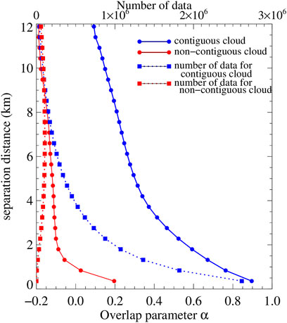
FIGURE 1. Globally-averaged α, the weighting (overlap) parameter regulating the mixing of maximum and random cloud occurrence overlap of two cloudy layers (α = 1: maximum overlap; α = 0: random overlap; α < 0: minimum overlap), as a function of separation distance Δz, derived from the O22 COD cloud fields. We show results for two cases, one where cloud is also encountered in all intervening layers (“contiguous cloud,” solid blue curve and circle symbols), and one where the intervening layers can contain clear skies (“non-contiguous cloud,” solid red curve and circle symbols). The number of data points used to derive the profiles for each case are shown with the dotted curves using the same color convention and square symbols.
Our analysis process is as follows. We first calculate α and ρ profiles for individual scenes. For two arbitrary cloud layers at levels n and m that are apart by a separation distance Δzn,m, the scene’s α for these two layers is calculated from:
where Cn,m is the true combined cloud fraction of layers n, m, calculated from the binary cloud fraction values (0 or 1) of the portion of the layer contained in subcolumn k.
K is the number of subcolumns in the scene (K = 100, in our case) and ck,n,m = 1 if either or both of n, m layers of the subcolumn are cloudy and ck,n,m = 0 when both are clear.
Spearman’s rank correlation coefficient ρ is calculated from:
where L is the number of subcolumns where both layers n and m have cloud, and rn,l and rm,l are the COD ranks of layers n and m for the l th subcolumn.
The separation distance Δz is resolved at 240 m, thus all separation distances are multiples of 240 m. Values for the same separation distance are averaged regardless of the vertical location of levels n and m, and we therefore drop henceforth layer subscripts from α, ρ, and Δz.
3 Overlap analysis
3.1 Cloud occurrence vertical overlap
Once α “profiles” (variations vs. Δz) are calculated at the scene level, they are averaged into multi-annual seasonal profiles at 4° latitudinal resolution by appropriate averaging the scene data by latitude
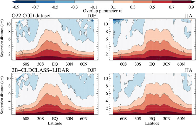
FIGURE 2. Zonal variation of mean α as a function of separation distance Δz for DJF (December - January-February), left panels, and JJA (June-July-August), right panels. The upper panels come from calculations using the O22 COD fields and the bottom panels from 2B-CLDCLASS-LIDAR. The latitudinal resolution is 4° and the vertical resolution used for the plot is 480 m.
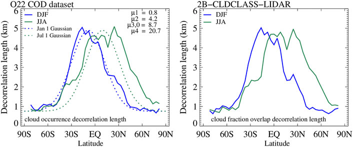
FIGURE 3. (Left panel): Zonal variation of the cloud occurrence decorrelation length parameter Lα, modulating the exponential decay of α vs. separation distance according to Eq. 2, for DJF and JJA from the O22 COD dataset; we also show Gaussian fits (dotted curves) corresponding to Eq. 7 with µ parameters provided on the top right corner for January 1st and July 1st. (Right panel): as the left panel, but from the cloud mask provided by the 2B-CLDCLASS-LIDAR product.
The prominent zonal dependence of α and the expected decrease with separation distance are immediately apparent in Figure 2. At the highest separation distance α approaches zero (random overlap) and can even become negative (some degree of minimum overlap). One should keep in mind that sampling becomes progressively poorer the greater the separation distance (cf. Figure 1), so results become noisier, but the tendency towards zero or negative values is clear and consisted with all previous overlap studies. The geographical dependence of α, with the higher values at low latitudes progressively decreasing at high latitudes is also consistent with previous works (Shonk et al., 2010; O12) where it was interpreted as indicative of the greater vertical alignment in cloud types encountered most frequently at low latitudes. Tompkins and Di Giuseppe (2015) casted however doubts on this interpretation arguing instead that the observed behavior rather reflected latitudinal changes in cloud scales (also related to latitudinally-varying frequencies of cloud types) relative to the fixed size of the scene for which α is calculated (∼110 km in our case).
A seasonal dependence of α is also apparent when comparing the DJF (December-January-February) and JJA (June-July-August) panels. The most distinguishing feature is the movement of high α values northward and the expansion of the latitude-height phase space area occupied by positive values of α in the summer hemisphere. Basically, at a given separation distance, there is greater chance to find a higher value of α in the summer hemisphere than the winter hemisphere. This reflects a tendency of greater likelihood of occurrence of vertically developed (and apparently more vertically aligned) clouds in the summer hemisphere than the winter hemisphere. In the tropics, the movement of the Intertropical Convergence Zone (ITCZ) is similarly reflected by higher values of α north of the equator during JJA.
The seasonal variation of α becomes more apparent when expressed in terms of decorrelation length. From the zonal profile of α, the zonal variation of its decorrelation length Lα can be calculated by applying a linear regression fit to lnα vs.–Δz data for which 1/Lα is simply the slope (Figure 3). This type of fit has been previously employed by Mace and Benson-Troth (2002) and Naud et al. (2008), among others, and results in a different Lα than the “effective” decorrelation length of Barker (2008b) and Jing et al. (2016) which is only meaningful at the scene level. Appropriate sampling weights are used in the regression fit to account for the fact that fewer values are available for larger Δz’s. Again, we show separate curves of Lα for DJF and JJA from the two datasets, the filled COD field (left panel) and 2B-CLDCLASS-LIDAR (right panel). To obtain the results shown in Figure 3, we actually calculated an Lα zonal curve separately for each year’s season (i.e., instead of calculating the seasonal average across 4-years) and then averaged the four year-specific Lα curves of each season. We opted to do this in order to suppress the over-smoothing of α profiles caused by extensive averaging (cf. Figure 1). The extreme flipside would have been to calculate Lα from very noisy α profiles of individual scenes (of which there are about four million) and averaging across the very large Lα population. The two methods, namely zonal Lα from fits to zonally-averaged α profiles and zonal Lα from averaging individual scene Lα’s yield different results. We do not opt for the second method because of the poor regression fits of individual scenes and the distorting effects a few extreme values can have. But even in our method which first conducts extensive averaging to α before calculating Lα, the quality of the regression has some dependence on latitude.
Zonal and seasonal contrasts in cloud occurrence overlap become the most apparent when overlap is expressed in terms of decorrelation length (Figure 3, solid curves). The peak values in Lα reach ∼5 km at the northern (JJA) and southern (DJF) edge of the tropics and drop quite rapidly towards mid and high latitudes. The contrast in Lα between the two seasons is much more pronounced in the NH than the SH. The two seasonal Lα zonal curves, the one coming from O22’s COD field (left panel of Figure 3), and the one from the standard 2B-CLDCLASS-LIDAR product (right panel of Figure 3) are very similar.
The magnitude of peak values of Lα is generally higher than in previous studies, although a direct comparison can only be conducted with O12. The reasons for the discrepancy with O12 are not entirely clear, but the different nature of the underlying dataset likely plays a significant role: α and Lα values in O12 were derived from a dataset based solely on CloudSat measurements, specifically a cloud mask inferred from 2B-GEOPROF reflectivities deemed to come from cells identified as cloudy according to predetermined thresholds. Here we use a daytime COD field, from combined CloudSat and CALIPSO measurements, and with retrievals available only when the algorithm converges to a solution. It is doubtful that the daytime aspect of the COD field explains the rather substantial discrepancy of decorrelation length values. Missing COD values being filled, and the specific method used to achieve this in O22 does not seem to be a factor either (left panel of Figure 4). Actually, had we not filled missing COD values we would have obtained even higher peak Lα values: because the filled values correspond to low (liquid) clouds, the chances of creating occurrences of overlap with high clouds increases; such overlaps tend towards random and correspond to lower Lα.
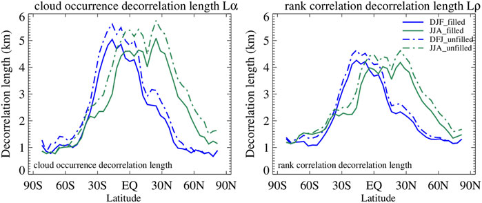
FIGURE 4. (Left panel): Zonal variation of Lα for DJF and JJA from the two versions of the O22 COD dataset, one unfilled (straight merging of 2B-CWC-RVOD and 2C-ICE COD fields) and one filled (to make consistent with 2B-CLDCLASS-LIDAR mask). (Right panel): as the left panel, but for Lρ.
For a practical use of the observed Lα values, the latitudinal and seasonal variability should ideally be captured by a parameterization. We follow here on the footsteps of O12 who used time-varying Gaussian functions whose parameters vary with Julian date (J), namely:
(we drop the subscript from L because this parameterization is also applied for COD overlap) where μ1, μ2, μ4 are constants, while μ3 varies with day of the year according to the equations below controlling the latitude at which the decorrelation length peaks:
Such a parameterization can be easily incorporated in a climate model that has a cloud subcolumn generator (Räisänen et al., 2004), as shown in O12. Figure 3 (dotted curves) shows the Gaussian curves for January 1st and July 1st and includes the parameters of the Gaussian fit. The present parameterization has the exact same functional form as the one introduced by O12 and encapsulates the migration of the most vertically aligned (and presumably developed) clouds (those with the highest value of Lα) northward (southward) during boreal summer (winter). The new parameters produce higher values of Lα (more maximum overlap) at low latitudes and smaller values (more random overlap) at high latitudes, compared to O12. In Section 4 we present an implementation of this parameterization to assess scene and grand-average simulated cloud properties and average cloud radiative effects and to evaluate the impact of transitioning from O12’s to the current Gaussian fits.
3.2 Cloud optical depth vertical overlap
The “profiles” (Δz dependences) of rank correlation coefficient ρ of COD distributions are calculated and averaged similarly to profiles of α. Figure 5 provides a visualization of the zonal dependence of ρ profiles for DJF and JJA as in Figure 2. We see a similar pattern for ρ(
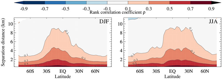
FIGURE 5. Zonal variation of mean ρ, the correlation coefficient of COD ranks between cloudy layers, as a function of their separation distance Δz, for DJF (left panel) and JJA (right panel) from the filled COD O22 dataset.
Estimates of Lρ are obtained by regressing ln(ρ) against -Δz, similarly to how we calculated Lα; namely by performing again a regression on each year’s seasonal zonal profiles, and averaging seasonal values across the 4 years. The zonal variation of Lρ for DJF and JJA is shown in Figure 6 (solid curves). The zonal pattern is very similar to that of Lα even though the cloud fraction overlap parameter and the rank correlation of COD are distinct physical parameters describing different aspects of cloud vertical structure. A model-oriented parameterization vs. latitude and day of the year is again accomplished with a Gaussian function of the same type as for Lα (Eq. 7), with parameter values included in Figure 6 which shows parameterized curves for January 1st and July 1st (dotted curves).
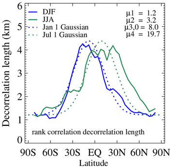
FIGURE 6. Zonal variation of the decorrelation length Lρ of the correlation coefficient ρ of COD ranks Lρ, modulating the exponential decay of ρ vs. separation distance according to Eq. 3, for DJF and JJA along with Gaussian fits according to Eq. 7 for January 1st and July 1st.
Because our COD filling procedure assigns equal values of liquid COD to cells when they belong to rays (cloudy subcolumns) where TAU from MODIS is available to be used as constraint, a tendency to overestimate ρ might have been expected. Such a potential overestimate implies higher values of Lρ which is however not seen; in reality the unfilled COD fields imply somewhat higher rank correlations (right panel of Figure 4). First of all, one should keep in mind that equal COD values in two different layers do not necessarily have the same rank. Second, the lower rank correlation of the filled COD field may be explained by the fact that many cells are filled by a secondary procedure that utilizes the available COD of neighboring liquid cells, and this process may actually increase randomness and therefore decrease rank correlations. Third, lower rank correlations can also result from an increase in the frequency of distant cloud layer pairs after filling, and such pairs are expected to have COD distributions that are more uncorrelated.
The peak magnitudes of Lρ at low latitudes are somewhat smaller than those of Lα, but at some higher latitudes the values of Lρ surpass those of Lα. This behavior differs from that in O12 where Lρ < Lα was universal, but with Lρ calculated directly from radar reflectivities of cloudy cells, and not actual cloud retrievals, and in Oreopoulos and Norris (2011) who used cloud condensate retrievals from ground-based radar. In an analysis of cloud resolving model (CRM) fields Pincus et al. (2005) found that Lρ > Lα is possible depending on the subset of clouds used and the method of calculation. Räisänen et al. (2004) in their own analysis of different CRM fields find Lρ < Lα consistently. O22 found that halving the magnitude Lα while at the same doubling the magnitude of Lρ compared to the original parameterization of O12 did not have serious undesired consequences on the radiative effects of cloud fields constructed by the Raisanen cloud subcolumn generator, which implies that Lρ > Lα is plausible and not necessarily unphysical.
3.3 Overlap dependences
3.3.1 Height of upper layer
In the previous analysis we derived a single decorrelation length for the entire atmospheric column. This is because we averaged α and ρ over all identical separation distances Δz regardless of cloud layer heights. Räisänen et al. (2004) on the other hand showed height-dependent decorrelation lengths (their Figure 3) obtained by solving Eqs. 2, 3 for adjacent layers, implying that overlap can be different for the same separation distance Δz at different parts of the atmosphere. Here we also attempt to resolve the dependence of the overlap parameters and their corresponding decorrelation lengths on height, but rather coarsely only. Specifically, we derive the zonal variation of decorrelation lengths for three different standard layers by segregating the calculations of α and ρ from Eqs. 4, 6 according to the location of the top of the upper cloud layer. The three standard layers are delineated by the 680 hPa and 440 hPa pressure levels separating clouds into low (L) when their cloud top pressure (CTP) is greater than 680 hPa, middle (M) if 440 hPa < CTP <680 hPa, and high (H) when CTP <440 hPa, as in the convention established by the International Satellite Climatology Project (ISCCP, Rossow and Schiffer 1999). CTPs were obtained from geometrical top heights with the help of the ECMWF-AUX CloudSat dataset. The range of possible Δz’s is highest when the top layer is H, and lowest when the top layer is L. This is because H clouds can be overlapped with H, M, and L clouds, and L clouds with only other L clouds; M clouds can be overlapped with other M clouds as well as with L clouds.
Figure 7 shows the zonal curves for both Lα and Lρ, for two seasons as before and segregated by cloud category according to the vertical location of the upper cloud layer. Aside from the previously noted seasonal zonal shifts, we also see a stronger dependence on the category assignment of the top cloud for cloud occurrence overlap (Lα) than COD overlap (Lρ). But even for Lα, the dependence on cloud category is more pronounced at low latitudes than high latitudes. More random overlap for the cases where the upper cloud is H makes sense because the overlap samples include higher separation distances for which overlap tends more towards random. But the same expectation based on this argument does not extend to the M vs. L comparison where separation distances are smaller, and where therefore less random overlap is expected, when the upper cloud layer belongs to the L category. It thus looks like there is an underlying physical reason (yet unknown) for more maximum overlap of cloud occurrence (and to a smaller degree of random correlation in COD ranks) within M clouds and for M clouds over L clouds.
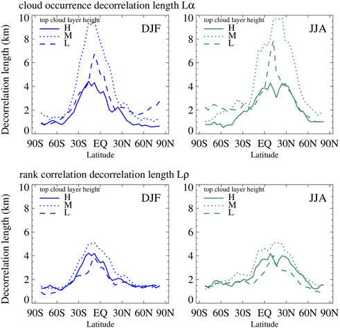
FIGURE 7. Zonal variation of Lα (top panels) and Lρ (bottom panels) for DJF (left panels) and JJA (right panels) when α and ρ are segregated according to the height category of the top layer (see text for details).
The breakdown of overlap according to the H, M, L category convention described here is simple enough to be included in a model that uses a subcolumn generator. Basically, the type of Gaussian fits previously discussed can be applied to the three broad cases where the upper cloud belongs to one of the three categories. Whether this additional level of nuance is called for instead of the simpler approach of obtaining decorrelation lengths without a height distinction would require testing.
3.3.2 Cloud regime
While the path to a relevant parameterization that can be applied to GCMs may turn out to be impractical and the ultimate impact small, it is worth pursuing a deeper understanding of cloud overlap by examining its dependence on cloud regime (CR). To accomplish this, we derived the zonal variation of decorrelation length by compositing separately within 4° latitude bands α and ρ for scenes coinciding with one of the Aqua MODIS CRs of Cho et al. (2021) which represent the dominant mixtures of clouds at 1° daily scales according to CTP-TAU joint histograms. Because many CRs have considerable geographical preference (see Cho et al., 2021 for CR descriptions and characteristics), sampling is not adequate across all latitudes, especially when the analysis is broken by season, as we have done so far. To improve sampling, we therefore combine some CRs into groups and create appropriate annual zonal averages of α and ρ before applying the regressions that yield Lα and Lρ; as before, the four annual values are averaged. The results of this procedure are shown in Figure 8; each panel also includes the zonal relative frequency of occurrence (RFO) of the combined (when applicable) CRs (dotted curves). The RFO curves reveal the geographical preference of CRs: CR1 and CR2 stand mainly for deep convection and cirrus, and are predominantly tropical cloud regimes, while CR3 and CR4 represent storms in both tropics and midlatitudes; CR5-CR6 (extratropical ocean storms and mid-level clouds often associated with orography) and CR7-CR9 (mostly oceanic stratus and stratocumulus) dominate mid and high latitudes, the low cloud fraction CR10 (oceanic shallow convection) is encountered mostly in the tropical/subtropical domain, while the even lower cloud fraction CR11 (mixture of low and high clouds) is omnipresent, and with a prominent peak in the southern polar regions. Decorrelation lengths are not calculated where sampling is poor. This is most notable for CR1-CR2 which do not have decorrelation lengths outside of 30° S-N, and for CR7-CR9 for which the decorrelation lengths have a gap north of the equator.
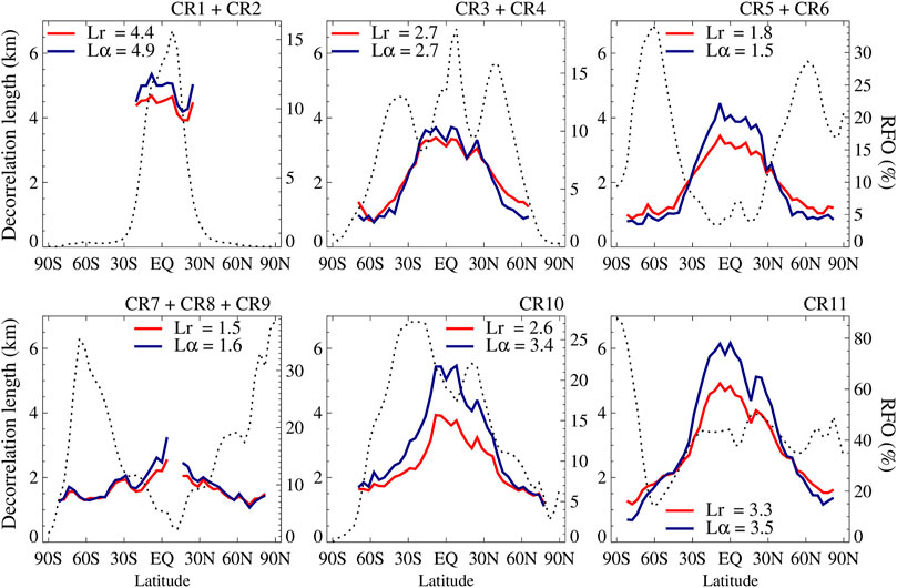
FIGURE 8. Annually averaged zonal curves of Lα and Lρ for groups of cloud regimes (CRs) from the O22 filled COD dataset; global average values are shown in each panel. These results are obtained by identifying the coincident Aqua-MODIS CR for each of our scenes and then deriving decorrelation lengths from zonal values of α and ρ for each CR group. The dotted curve indicates the zonal Relative Frequency of Occcurrence (RFO, in %, right ordinate) of the CR group.
For regimes where a near-full zonal distribution of decorrelation length can be calculated (all CRs except CR1 and CR2), the previously seen zonal behavior re-emerges, namely higher decorrelation lengths at low latitudes (tropics and subtropics). With regard to peak values, the CRs seem to be broadly separated into two groups, one with peak values of Lα around 5–6 km (CR1+CR2, CR10, CR11) and one with peak values roughly 2 km lower (CR3-CR9), although in the case of CR5-CR9 the peaks also correspond to the lowest number of samples. The first class is dominated by either deep or high clouds (CR1 + CR2) or scenes of small cloud fraction (CR10 and CR11). The second class (CR3-CR9) encompasses all remaining storm and low clouds. Despite the uneven sampling, these results suggest that the low latitude members of cloud systems deemed to belong to the same family as their extratropical brethren based on resemblance of CTP-TAU histograms (the measure of similarity in MODIS cloud regime classification) exhibit nevertheless distinct overlap behavior. This result seems to counter the Tompkins and Di Giuseppe (2015) argument that overlap metrics are skewed by the relative sizes of cloud objects and domain sizes. Here, for a fixed domain size and cloud objects presumably of similar size given their membership to the same CR (a plausible, but not rigorous assumption), we see vertical overlap to differ quite substantially between low and high latitudes.
The correlation of COD ranks expressed in terms of Lρ seems to also follow the zonal pattern seen previously and to trace closely Lα, but at slightly smaller magnitudes, per the earlier results. The global values of the two decorrelation lengths included in the Figure 8 panels reaffirm the close proximity noticed earlier. CR1 + CR2 assume the greatest decorrelation length magnitudes, and CR5-CR9 the lowest. The large gap in magnitude between these two broad cloud groups is a striking indicator of how varied the cloud overlap of the planet’s clouds can be, and how much detail is missed when the analysis is performed indiscriminately on all clouds.
4 Performance of parameterized overlap
In this section we discuss practical implementations of the findings of the preceding overlap analysis. Specifically, we use the updated decorrelation length parameterizations (Eq. 7) in the “Raisanen generator” (Räisänen et al., 2004) to produce for each 100-ray scene subcolumns that are then filtered through the COSP [CFMIP (Cloud Feedback Model Intercomparison Project) Observation Simulator Package, Bodas-Salcedo et al., 2011] MODIS simulator to produce for each scene a simulated 2D COD field that is consistent, to the extent possible, with MODIS retrievals of TAU (vertical integral of subcolumn COD) and CTP (pressure of what MODIS would consider the cloud top of the subcolumn). As part of this process, subcolumns with TAU <0.3 are discarded and scene cloud fraction is resolved in terms of CTP-TAU joint histograms as in O22.
We first assess the performance of the generator with the new decorrelation length parameterization at the scene level (for reasons explained in O22 only oceanic scenes are used) and also compare with results obtained using the O12 parameterization. For each scene, values of Lα and Lρ are calculated from the parameterization using the center latitude of the scene and the Julian date on which it was observed. Results are shown in Figure 9 which employs density plots to contrast observed scene vertically projected cloud fraction, mean logarithm of TAU and variance of TAU (also from the MODIS simulator) against two versions of their simulated counterparts, one using O12’s parameterization of decorrelation lengths and another using the updated version of this paper in the Raisanen generator. Figure 9 reveals that the new parameterizations of decorrelation lengths (the parameterization of layer COD variance remains the same as in O12, namely a beta COD distribution with variance parameterized as a function of layer cloud fraction) do not yield tangible improvements over the old parameterization. While the performance in terms of mean values is slightly better (as indicated by the smaller mean errors provided in the panels), correlations and RMSEs are either the same or slightly inferior.
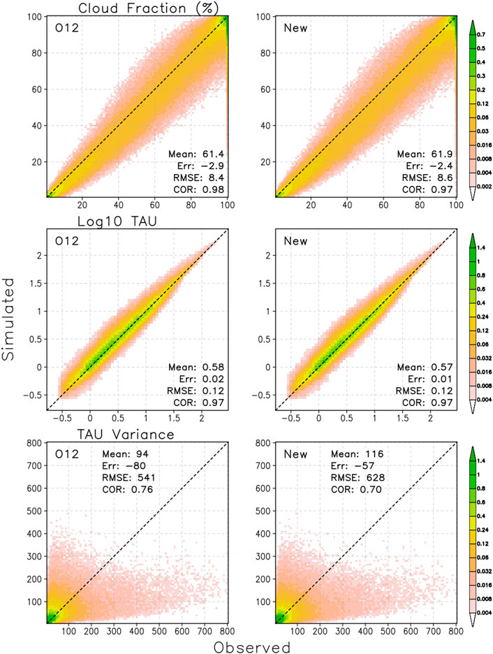
FIGURE 9. Comparison of the performance of the O12 (panels is left column) and the present (panels in right column) decorrelation length parameterization at the level of individual scenes simulated with the Raisanen subcolumn generator. Occurrence frequencies are shown for combinations of observed and simulated vertically projected scene cloud fraction CF (top row), the logarithm of vertically integrated optical depth log (TAU) (middle row), and the variance of the vertically integrated optical depth var (TAU) (bottom row).
A performance comparison of decorrelation length parameterizations was also conducted in terms of CTP-TAU joint histograms. The scene level results are shown in Figure 10. The left panel shows Euclidean Distances (EDs, square root of the sum of squared bin CF differences) between the joint histograms of observed and simulated scenes composited in terms of scene cloud fraction. The smaller the ED, the more similar the observed and simulated joint histograms are (i.e., better performance). The mean ED of the new parameterization is slightly larger indicating a marginally worse performance. The density plot of scene level ED values (right panel) is nearly symmetric around the line of perfect agreement indicating that the performance of the two parameterizations is practically equivalent.
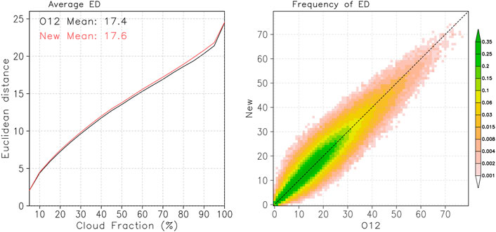
FIGURE 10. Comparison of the performance of the O12 and the present decorrelation length parameterization at the scene level. Average Euclidean Distance (ED) as a function of scene CF (binned in 5% intervals, (left panel); occurrence frequency of pairs of ED values obtained from the O12 and current parameterization of decorrelation lengths (binned in 1% intervals, (right panel).
A more straightforward comparison is that of grand-averages of observed and simulated joint histograms. This is shown in Figure 11 and confirms the slight edge of the new parameterization on average. The grand-averaged joint histogram of the new parameterization is slightly more similar to its observed counterpart as evidenced by a smaller ED and a closer to observations vertically projected cloud fraction (albeit still substantially far from the observed value).
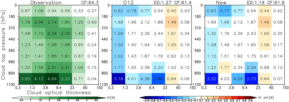
FIGURE 11. Grand-average of CTP-TAU oceanic CF histograms from observations (O22 COD filled, left panel), simulated with the Raisanen simulator using the decorrelation length Gaussian fits of O12 (middle panel) and the new Gaussian fits of this paper (Figures 3, 6) (right panel).
Does the marginal improvement brought by the new parameterization in a mean sense matter radiatively? We found that it does not. We examined this in the same way as O22 by converting joint CTP-TAU histograms to shortwave (SW), longwave (LW) and total = SW + LW Cloud Radiative Effect (CRE) resolved in CTP-TAU space using observation-based Cloud Radiative Kernels from the Clouds and the Earth’s Radiant Energy System (CERES) FluxByCldTyp product (Sun et al., 2022); details of the methodology can be found in O22. Results are shown in Figure 12 and once again reaffirm how negligible the performance differences between the two parameterizations are. The most important conclusion actually does not pertain so much to differences between the two parameterizations, but rather to how well the implementation of this type of parameterization into the Raisanen generator reproduces CREs on average, both in terms of the overall value, but also in terms of the distribution itself of average binned CRE.
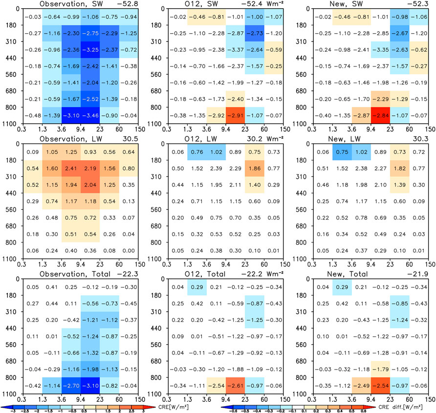
FIGURE 12. SW (top row) LW (middle row) and total = SW + LW (bottom row) CRE discretized by combinations of CTP-TAU bins when using CF joint histograms from observations, and the Raisanen generator with either the O12 decorrelation length parameterization or the parameterization of this paper. The colors in the left column correspond to the actual CRE binned values numbers while in the other two columns to differences from observations.
5 Conclusion and perspectives on cloud vertical overlap
Taking advantage of the availability of new datasets from CloudSat’s radar and CALIPSO’s lidar, we have re-evaluated parameters used to describe vertical cloud overlap at ∼ 100 km scales. Specifically, we used COD fields created in recent work (Oreopoulos et al., 2022). When expressing the vertical overlap of cloud occurrences and of COD distributions in terms of decorrelation lengths as is common in the cloud overlap literature, we found larger peak values than in previous work also based on CloudSat and CALIPSO observations (Oreopoulos et al., 2012). We also took the opportunity to extend that work by examining overlap in more detail for different cloud classes. In particular, we examined how overlap contrasts among broad categories of high, middle, and low clouds, but also among more finely-defined cloud categories based on passive observations, known as cloud regimes. All such overlap breakdowns showed an unambiguous zonal pattern for both cloud occurrence and cloud optical depth overlap decorrelation lengths with clear peaks at low latitudes indicating more aligned vertical structures, possibly due to stronger large-scale vertical motions and less wind shear (Di Giuseppe and Tompkins 2015) in the tropics and subtropics. They also showed that an analysis that ignores cloud classes conceals a great amount of diversity in how the planet’s clouds overlap.
For a practical use of our overlap analysis we applied the same type of Gaussian fits to the observed zonal curves of the two decorrelation lengths as in O12 and then implemented the updated parameterization in the “Raisanen generator” (Räisänen et al., 2004) to produce subcolumns that form simulated scenes. From these subcolumns, COSP’s MODIS simulator generates subcolumn CTP and TAU values as well as subgrid distributions of cloud fraction in terms of CTP-TAU joint histograms. These quantities were then be compared with their observational counterparts obtained by similarly passing the observed COD field through the MODIS simulator. This exercise showed no notable performance enhancements compared to the case where O12 decorrelation length parameterizations were used.
The above major finding raises the question of how sensitive the performance (as evaluated here) of subcolumn generation is to extreme values of decorrelation length. We tested this by implementing unrealistic maximum and random overlap (decorrelation lengths of infinity and zero, respectively) for both cloud occurrence and COD distribution overlap, specifically the four possible combinations of purely maximum and purely random overlap for the two types of overlap. Results are shown in Figure 13. We see that neither maximum nor random overlap works in any combination, as it yields large errors in CTP-TAU histograms. As expected, random cloud occurrence overlap produces big overall estimates of cloud fraction, which are more extreme when COD overlap is also random because in that case the likelihood of TAU <0.3 decreases. An overall overestimation in total projected cloud fraction (CF) does not mean that CF is overestimated in every histogram bin. This is because random overlap also decreases the likelihood of extensive vertical alignment that creates optically thick clouds. When on the other hand Lα = ∞, i.e., cloud occurrence overlap is maximum, overall CF is underestimated, less so than when COD overlap is random, because of more TAU >0.3 subcolumns. Again, individual histogram bins that go against the underestimation expectation exist. This is because maximum overlap also creates pockets of more populous than observed optically thicker clouds. While pure maximum and pure random overlap perform very poorly, when combined as in the original maximum-random paradigm described in the introduction and implemented in COSP’s SCOPS (Subcolumn Cloud Overlap Profile Sampler) subcolumn generator, performance is acceptable, albeit inferior to that of generalized overlap (see O22).
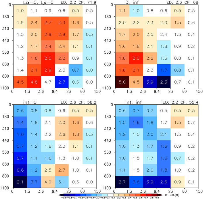
FIGURE 13. Mean CF errors discretized in CTP-TAU bins (i.e., joint histogram errors) for four combinations of extreme Lα and Lρ. Zero values correspond to random vertical overlap of cloud fraction and COD ranks, while infinite values correspond to maximum cloud fraction overlap and perfect correlations of COD ranks.
A survey of the overlap literature exploring generalized overlap since 2000 when the Hogan and Illingworth (2000) work was published, reveals that decorrelation length magnitudes capturing the decay of the parameter α controlling the mixing of maximum and random overlap occupy an enormous range that makes convergence towards universally accepted values for GCM parameterization purposes challenging (rank correlation of distributions of condensate or optical depth have been studied much less). Magnitudes of decorrelation length depend on exact definitions (e.g., the “effective” decorrelation length of Barker 2008b, while similar, does not have the same meaning as in the original definition adopted here); the type of dataset used (cloud fields simulated by a cloud resolving model, ground-based radar, space-based radar, combined space-based radar-lidar observations); the size of the reference domain (scene); the cloud fraction threshold used to weed out non-meaningful calculations of overlap; types of clouds examined or retained for overlap calculations; whether only contiguous or all cloudy layers are used, or whether only adjacent cloud layers are used; and how the values of either α and Lα are sampled, averaged, fitted, and composited. Given this multitude of dependences and some degree of insensitivity to Lα in the end values of cloud and radiation statistics, one is left wondering how modelers can chose the most appropriate decorrelation length values. Our results show that both the Oreopoulos et al. (2012) and the new parameterization derived here are viable, at least in a mean sense (substantial errors at the scene level are still not universally suppressed). They also make apparent that a latitudinal dependence of decorrelation length is an essential aspect of a parameterization, preferably also accounting for seasonal variation. If GCMs still perform long integrations with rather coarse grids in the near future, cloud vertical overlap remains an important observable that should be periodically revisited with improved active observations and cloud products such as those expected in a few years from NASA’s Atmospheric Observing System (AOS) and ESA’s EarthCare mission.
Data availability statement
MODIS and CERES data were obtained from www.earthdata.nasa.gov, CloudSat/CALIPSO data from www.cloudsat.cira.colostate.edu, MODIS Cloud regimes from https://disc.gsfc.nasa.gov; further inquiries can be directed to the corresponding author.
Author contributions
LO conceived the study and analysis methods, and led authorship of the manuscript. NC constructed the satellite dataset and performed the observational analysis. DL performed the simulations to evaluate performance of parameterization. Both NC and DL created figures and contributed to the authorship of the manuscript.
Funding
This study was supported by the NASA’s CloudSat-CALIPSO Science Team program under David Considine. Resources supporting this work were provided by the NASA High-End Computing (HEC) Program through the NASA Center for Climate Simulation (NCCS) at Goddard Space Flight Center.
Conflict of interest
The authors declare that the research was conducted in the absence of any commercial or financial relationships that could be construed as a potential conflict of interest.
Publisher’s note
All claims expressed in this article are solely those of the authors and do not necessarily represent those of their affiliated organizations, or those of the publisher, the editors and the reviewers. Any product that may be evaluated in this article, or claim that may be made by its manufacturer, is not guaranteed or endorsed by the publisher.
References
Barker, H. W. (2008a). Overlap of fractional cloud for radiation calculations in GCMs: A global analysis using CloudSat and CALIPSO data. J. Geophys. Res. 113, D00A01. doi:10.1029/2007JD009677
Barker, H. W. (2008b). Representing cloud overlap with an effective decorrelation length: An assessment using CloudSat and CALIPSO data. J. Geophys. Res. 113, D24205. doi:10.1029/2008JD010391
Bodas-Salcedo, A., Webb, M. J., Bony, S., Chepfer, H., Dufresne, J. L., Klein, S. A., et al. (2011). COSP: Satellite simulation software for model assessment. Bull. Am. Meteorological Soc. 92 (8), 1023–1043. doi:10.1175/2011BAMS2856.1
Cho, N., Tan, J., and Oreopoulos, L. (2021). Classifying planetary cloudiness with an updated set of MODIS cloud regimes. J. Appl. Meteorology Climatol., 60(7), pp.981–997. doi:10.1175/JAMC-D-20-0247.1
Chou, M. D., Lee, K. T., Tsay, S. C., and Fu, Q. (1999). Parameterization for cloud longwave scattering for use in atmospheric models. J. Clim., 12(1), pp.159–169. doi:10.1175/1520-0442(1999)012<0159:PFCLSF>2.0.CO;2
Chou, M. D., Suarez, M. J., Ho, C. H., Yan, M. M., and Lee, K. T. (1998). Parameterizations for cloud overlapping and shortwave single-scattering properties for use in general circulation and cloud ensemble models. J. Clim., 11(2), pp.202–214. doi:10.1175/1520-0442(1998)011<0202:pfcoas>2.0.co;2
Di Giuseppe, F., and Tompkins, A. M. (2015). Generalizing cloud overlap treatment to include the effect of wind shear. J. Atmos. Sci. 72 (8), 2865–2876. doi:10.1175/JAS-D-14-0277.1
Geleyn, J. F., and Hollingsworth, A. (1979). An economical analytical method for the computation of the interaction between scattering and line absorption of radiation. Contrib. Atmos. Phys. 52, 1–16.
Hillman, B. R., Marchand, R. T., and Ackerman, T. P. (2018). Sensitivities of simulated satellite views of clouds to subgrid-scale overlap and condensate heterogeneity. J. Geophys. Res. Atmos., 123(14), pp.7506–7529. doi:10.1029/2017JD027680
Hogan, R. J., and Illingworth, A. J. (2000). Deriving cloud overlap statistics from radar. Q. J. R. Meteorological Soc., 126(569), pp.2903–2909. doi:10.1002/qj.49712656914
Jing, X., Zhang, H., Peng, J., Li, J., and Barker, H. W. (2016). Cloud overlapping parameter obtained from CloudSat/CALIPSO dataset and its application in AGCM with McICA scheme. Atmos. Res. 170, 52–65. doi:10.1016/j.atmosres.2015.11.007
Mace, G. G., and Benson-Troth, S. (2002). Cloud-layer overlap characteristics derived from long-term cloud radar data. J. Clim. 15 (17), 2505–2515. doi:10.1175/1520-0442(2002)015<2505:clocdf>2.0.co;2
Naud, C. M., Del Genio, A., Mace, G. G., Benson, S., Clothiaux, E. E., and Kollias, P. (2008). Impact of dynamics and atmospheric state on cloud vertical overlap. J. Clim. 21 (8), 1758–1770. doi:10.1175/2007JCLI1828.1
Oreopoulos, L., Cho, N., Lee, D., Lebsock, M., and Zhang, Z. (2022). Assessment of two stochastic cloud subcolumn generators using observed fields of vertically resolved cloud extinction. J. Atmos. Ocean. Technol. 39 (8), 1129–1244. doi:10.1175/JTECH-D-21-0166.1
Oreopoulos, L., and Khairoutdinov, M. (2003). Overlap properties of clouds generated by a cloud-resolving model. J. Geophys. Res. Atmos. 108 (D15), 4479. doi:10.1029/2002JD003329
Oreopoulos, L., Lee, D., Sud, Y. C., and Suarez, M. J. (2012). Radiative impacts of cloud heterogeneity and overlap in an atmospheric General Circulation Model. Atmos. Chem. Phys., 12(19), pp.9097–9111. doi:10.5194/acp-12-9097-2012
Oreopoulos, L., and Norris, P. M. (2011). An analysis of cloud overlap at a midlatitude atmospheric observation facility. Atmos. Chem. Phys., 11(12), pp.5557–5567. doi:10.5194/acp-11-5557-2011
Pincus, R., Hannay, C., Klein, S. A., Xu, K. M., and Hemler, R. (2005). Overlap assumptions for assumed probability distribution function cloud schemes in large-scale models. J. Geophys. Res. Atmos., 110, D15S09(D15). doi:10.1029/2004JD005100
Räisänen, P., Barker, H. W., Khairoutdinov, M. F., Li, J., and Randall, D. A. (2004). Stochastic generation of subgrid-scale cloudy columns for large-scale models. Q. J. R. Meteorological Soc. A J. Atmos. Sci. Appl. meteorology Phys. Oceanogr., 130(601), pp.2047–2067. doi:10.1256/qj.03.99
Rossow, W. B., and Schiffer, R. A. (1999). Advances in understanding clouds from ISCCP. Bull. Am. Meteorological Soc. 80 (11), 2261–2287. doi:10.1175/1520-0477(1999)080<2261:aiucfi>2.0.co;2
Shonk, J. K., Hogan, R. J., Edwards, J. M., and Mace, G. G. (2010). Effect of improving representation of horizontal and vertical cloud structure on the Earth's global radiation budget. Part II: The global effects. Q. J. R. Meteorological Soc., 136(650), pp.1205–1215. doi:10.1002/qj.646
Sun, M., Doelling, D. R., Loeb, N. G., Scott, R. C., Wilkins, J., Nguyen, L. T., et al. (2022). Clouds and the Earth’s radiant Energy system (CERES) FluxByCldTyp edition 4 data product. J. Atmos. Ocean. Technol. 39 (3), 303–318. doi:10.1175/JTECH-D-21-0029.1
Tompkins, A. M., and Di Giuseppe, F. (2015). An interpretation of cloud overlap statistics. J. Atmos. Sci., 72(8), pp.2877–2889. doi:10.1175/JAS-D-14-0278.1
Keywords: active observations, cloud overlap, cloud radiative effects, subgrid variability, decorrelation length
Citation: Oreopoulos L, Cho N and Lee D (2022) Revisiting cloud overlap with a merged dataset of liquid and ice cloud extinction from CloudSat and CALIPSO. Front. Remote Sens. 3:1076471. doi: 10.3389/frsen.2022.1076471
Received: 21 October 2022; Accepted: 12 December 2022;
Published: 22 December 2022.
Edited by:
Seiji Kato, Langley Research Center (NASA), United StatesReviewed by:
Thibault Vaillant de Guélis, Langley Research Center (NASA), United StatesHartwig Deneke, Leibniz Institute for Tropospheric Research (LG), Germany
Howard Barker, Environment and Climate Change Canada (ECCC), Canada
Copyright © 2022 Oreopoulos, Cho and Lee. This is an open-access article distributed under the terms of the Creative Commons Attribution License (CC BY). The use, distribution or reproduction in other forums is permitted, provided the original author(s) and the copyright owner(s) are credited and that the original publication in this journal is cited, in accordance with accepted academic practice. No use, distribution or reproduction is permitted which does not comply with these terms.
*Correspondence: Lazaros Oreopoulos, TGF6YXJvcy5PcmVvcG91bG9zQG5hc2EuZ292
 Lazaros Oreopoulos
 Nayeong Cho
 Dongmin Lee