 Maninder Singh Dhillon1*
 Thorsten Dahms1Carina Kuebert-Flock2Thomas Rummler3Joel Arnault4Ingolf Steffan-Dewenter5
 Tobias Ullmann1
- 1Institute of Geography and Geology, Department of Remote Sensing, University of Wuerzburg, Wuerzburg, Germany
- 2Hessen State Agency for Nature Conservation, Environment and Geology, Department of Remote Sensing Hlnug, Wiesbaden, Germany
- 3Institute of Geography, Department of Applied Computer Science, University of Augsburg, Augsburg, Germany
- 4Institute of Meteorology and Climate Research, Campus Alpine, Karlsruhe Institute of Technology, Garmisch-Partenkirchen, Germany
- 5Department of Animal Ecology and Tropical Biology, University of Wuerzburg, Wuerzburg, Germany
The fast and accurate yield estimates with the increasing availability and variety of global satellite products and the rapid development of new algorithms remain a goal for precision agriculture and food security. However, the consistency and reliability of suitable methodologies that provide accurate crop yield outcomes still need to be explored. The study investigates the coupling of crop modeling and machine learning (ML) to improve the yield prediction of winter wheat (WW) and oil seed rape (OSR) and provides examples for the Free State of Bavaria (70,550 km2), Germany, in 2019. The main objectives are to find whether a coupling approach [Light Use Efficiency (LUE) + Random Forest (RF)] would result in better and more accurate yield predictions compared to results provided with other models not using the LUE. Four different RF models [RF1 (input: Normalized Difference Vegetation Index (NDVI)), RF2 (input: climate variables), RF3 (input: NDVI + climate variables), RF4 (input: LUE generated biomass + climate variables)], and one semi-empiric LUE model were designed with different input requirements to find the best predictors of crop monitoring. The results indicate that the individual use of the NDVI (in RF1) and the climate variables (in RF2) could not be the most accurate, reliable, and precise solution for crop monitoring; however, their combined use (in RF3) resulted in higher accuracies. Notably, the study suggested the coupling of the LUE model variables to the RF4 model can reduce the relative root mean square error (RRMSE) from −8% (WW) and −1.6% (OSR) and increase the R2 by 14.3% (for both WW and OSR), compared to results just relying on LUE. Moreover, the research compares models yield outputs by inputting three different spatial inputs: Sentinel-2(S)-MOD13Q1 (10 m), Landsat (L)-MOD13Q1 (30 m), and MOD13Q1 (MODIS) (250 m). The S-MOD13Q1 data has relatively improved the performance of models with higher mean R2 [0.80 (WW), 0.69 (OSR)], and lower RRMSE (%) (9.18, 10.21) compared to L-MOD13Q1 (30 m) and MOD13Q1 (250 m). Satellite-based crop biomass, solar radiation, and temperature are found to be the most influential variables in the yield prediction of both crops.
1 Introduction
Accurate crop monitoring in response to climate change at a regional scale plays a significant role in developing agricultural policies, improving food security, forecasting, and analyzing global trade trends (Jeong et al., 2016). The emergence of new technologies, such as simulation crop growth models (CGMs) and machine learning (ML), to synthesize and analyze large-scale data with high computing performance has increased the ability to accurately predict crop yields (Archontoulis et al., 2020; Bogard et al., 2020; Ersoz et al., 2020; Shahhosseini et al., 2020; Washburn et al., 2020). These technologies have each provided unique capabilities and significant advancements in prediction performance; however, they have been mainly assessed separately, and there may be benefits in integrating them to increase further prediction accuracy (Daw et al., 2017; Shahhosseini et al., 2021).
Since the 1960s, CGMs have reached a high degree of success in simulating the behaviour of real crops (i.e., by predicting their final state of total biomass or harvestable yield) (Dhillon et al., 2020). CGMs are a set of mathematical equations pre-trained using a diverse set of experimental data from various environments and are further refined (or calibrated) for more accurate predictions in each study (Kasampalis et al., 2018). They are increasingly applied as tools for decision-making and research, providing quantitative and temporal information on plant growth and development by including the effect of various climate variables (Mirschel et al., 2004; Murthy, 2004). Because CGMs lack spatial information, many studies have used them for forecasting applications by integrating them with remote sensing (RS) data (Clevers et al., 2002). The RS technology provides synoptic, timely, repetitive, and cost-effective information about the surface of the Earth (Justice et al., 2002; Ali et al., 2022); however, the cloud and shadow gaps in the optical satellite data can hinder or limit CGMs from producing accurate yield results (Roy et al., 2008; Gevaert and García-Haro, 2015). To fill the data gaps, many studies have successfully used multitemporal data fusion, combining the data obtained from two different sensors of different spatial and temporal scales (Benabdelouahab et al., 2019; Htitiou et al., 2019; Dhillon et al., 2020; Lebrini et al., 2020). Due to its public availability of code and simplicity of usage, the spatial and temporal adaptive reflectance fusion model (STARFM) (Gao et al., 2006) is widely used to combine Landsat or Sentinel-2 with the Moderate Resolution Imaging Spectroradiometer (MODIS) (Xie et al., 2016; Zhu et al., 2017; Cui et al., 2018; Lee et al., 2019). Numerous studies successfully utilized the multi-temporal data fusion for deriving the leaf area index (LAI), or fraction of absorbed photosynthetically active radiation (FPAR) obtained from vegetation indices, e.g., the normalized difference vegetation index (NDVI), in combination with CGMs to estimate crop biomass or yield in different study regions around the world (Hwang et al., 2011; Bhandari et al., 2012). Similarly, many studies have compared the performance of different CGMs by implementing them on the same crop and in the same study region (Eitzinger et al., 2004; Dhillon et al., 2020). For example, in the preceding work, we compared five CGMs for simulating the biomass of selected winter wheat (WW) fields in the federal state of Mecklenburg-West Pomerania in northeast Germany. We found that the AquaCrop and semi-empiric Light Use Efficiency (LUE) are highly applicable and precise than the WOFOST, CERES-Wheat, and CropSyst (Dhillon et al., 2020).
Even though CGMs have a reasonable prediction accuracy, they are not readily applicable due to the data calibration requirements, long runtimes, and data storage constraints (Drummond et al., 2003; Puntel et al., 2016; Shahhosseini et al., 2019). Moreover, their specified designs restrict them to considering only limited climate parameters, whereas the other essential climate elements were neglected, which might benefit from further increasing the prediction accuracy. On the other hand, ML models can deal with linear and non-linear relationships by obtaining quality results with lower runtimes–plus, they can input a vast range of climate elements, likely positively affecting the accuracy of crop yields (De’ath and Fabricius, 2000). Moreover, they are easy to implement as they usually provide a less complex calibration and have fewer data storage constraints (Shahhosseini et al., 2019). Numerous ML algorithms (such as linear regression, decision tree, and random forest (RF)) were applied to the RS data for the prediction of agronomic variables (Basso and Liu, 2019; Khaki and Wang, 2019; Haque et al., 2020; Khaki et al., 2020). Exemplary, the RF is a non-parametric advanced classification and regression tree (CART) analysis method that has been researched widely in many scientific fields. Most applications of RF have been focused on its utility as a classification tool with only limited studies exploring its regression capabilities for predicting crop yields (Vincenzi et al., 2011; Mutanga et al., 2012; Fukuda et al., 2013). However, some studies found that the RF could overfit data, making it unstable for crop yield estimation (Breiman, 2001; Segal, 2004). Moreover, RF could partially depend on variables of less importance that might affect the prediction accuracy negatively (Jeong et al., 2016). Therefore, coupling ML models with CGMs could be tested by training an RF model with the output of a crop model so that the RF can have the potential of overfitting issues within the range of training data.
Many studies have combined CGMs with simple regression models; however, to our knowledge, there are rare studies systematically investigating the effect of coupling ML and CGMs (Shahhosseini et al., 2021). The present study hypothesized that merging CGMs with ML models will improve yield prediction accuracy by combining the spatial crop biomass output of the LUE model (considered the most accurate, precise, and reliable (Dhillon et al., 2020)) with the RF model for WW and oil seed rape (OSR) in Bavaria. For this study, different RF models (RF1 (input: NDVI), RF2 (input: climate variables), RF3 (input: Normalized Difference Vegetation Index (NDVI) + climate variables), RF4 (input: LUE generated biomass + climate variables), and one semi-empiric LUE model were designed with different input requirements to find the best predictors of crop monitoring. In addition, the study investigates the accuracy of model outputs based on the spatial resolution of the RS products (without cloud and shadow gaps) inputting two STARFM-derived synthetic NDVI products (Landsat (L)-MOD13Q1 (30 m, 8 days) and Sentinel-2 (S)-MOD13Q1 (10 m, 8 days and one real NDVI product (MOD13Q1 (250 m, days)) (Dhillon et al., 2022). The specific research objectives include:
(i) Explore whether only NDVI (RF1) or climate elements (RF2) or both NDVI and climate elements (RF3) are the best predictors of crop monitoring using RF models;
(ii) Investigate the performance of LUE alone and its coupling with RF (RF4) for crop yield prediction of WW and OSR;
(iii) Highlight the effect of different spatial scales (10 or 30 or 250 m) for crop yield estimation.
2 Materials and methods
The study’s general workflow shows the input criteria for four different RF models (RF1, RF2, RF3, and RF4) and one LUE model designed to calculate the crop yield for Bavaria in 2019 (Figure 1).
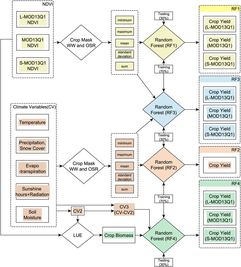
FIGURE 1. Conceptual framework of the study that explains the methodology of four random forest (RF1, RF2, RF3, and RF4) models with different input requirements to predict crop yield for winter wheat (WW) and oil seed rape (OSR). The semi-empiric light use efficiency (LUE) model is coupled with the RF4 model. CV belongs to climate variables and CV2 are the set of CV required by the LUE model. CV3 (CV minus CV2) are the set of CV required by the RF4 model. Landsat(L)-MOD13Q1, Sentinel-2(S)-MOD13Q1, and MOD13Q1 are the satellite inputs [generated by (Dhillon et al., 2022)].
Firstly, the pixel level satellite and climate inputs are masked out for every field of every region of Bavaria using the InVeKos data (source: www.ec.europa.eu/info/index_en) for WW and OSR. Secondly, the spatiotemporal-metrics (STMs) [such as minimum, maximum, mean, standard deviation (sd) and sum] for pixel-based time series (between the SOS and the EOS of WW and OSR) are calculated for every field. Then the field values are integrated at a regional level.
The STMs of NDVI data and climate elements are inputted into respective RF models in the following steps. The NDVI is the only spatial input for the RF1, whereas the yield output of the model is tested at different spatial resolutions of 10, 30, and 250 m. Similarly, the climate variables (CV) are used as input for the RF2 model. The RF3 model combines satellite NDVI and CV and tests the yield prediction at different spatial scales. Prior to that, LUE model results of crop yield are generated by inputting NDVI data and climate elements (CV2) required by the model. In the last steps, the LUE model (crop biomass as an input) is linked with the RF4 model. As CV2 is already inputted in the LUE model, for RF4, CV3 (CV2 are subtracted from the CV) is used as an input. The study’s main objective is to test the performance by coupling the crop simulation model and machine learning; therefore, the LUE model is coupled with the RF4 model, and the crop yield performance is tested for different satellite products.
All RF models are trained with 70% and tested with 30% of the crop yield data available at the regional level for both WW and OSR from the legal authorities [(i.e., Bayerisches Landesamt für Statistik (LfStat)]. Two synthetic (L-MOD13Q1: 30 m and 8-day; S-MOD13Q1: 10 m and 8-day) and one real-time (MOD13Q1: 250 m and 8-day) satellite NDVI time series [completed in preceding work (Dhillon et al., 2022)] is used as an input criterion for the RF and LUE models. The input NDVI and the climate data are selected for the respective start of the season (SOS) and end of the season (EOS) for WW and OSR in 2019.
2.1 Study area
The study region is the federal state of Bavaria located between 47˚N and 50.5˚N, and between 9˚E and 14˚E, in the southeastern part of Germany (Figure 2). The climate of the region is influenced by the region’s topography, with higher elevations in the south (northern edge of the Alps) and east (Bavarian Forest and Fichtel Mountains). The mean annual precipitation sums range from approx. 500 to above 3100 mm, with wetter conditions in the southern parts of Bavaria. The mean annual temperature ranges from −3.3°C to 11°C, but in most the regions, the temperature ranges between 8°C and 10°C (Dhillon et al., 2022). As the largest state in Germany, Bavaria covers an area of approx. 70,500 km2, covering almost one-fifth of Germany. The federal state is divided into 96 counties with 71 rural districts (so-called “Landkreise”) and 25 city districts (so-called “Kreisfreie Städte”). For the year 2019, the landcover of Bavaria covers 31.56% of the area under agriculture (Dhillon et al., 2022).
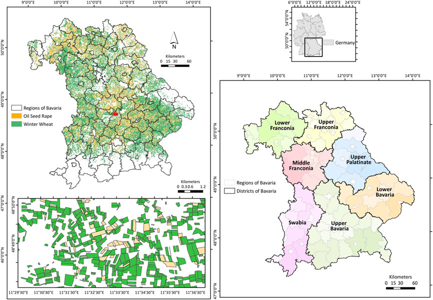
FIGURE 2. Overview of the study region with spatial information of winter wheat (WW) and oil seed rape (OSR) fields (left). The dark green color shows the fields of WW and dark orange shows the fields of OSR in 2019. The enlargement (displayed with a dark red box on the top left map) shows the detailed version of WW and OSR fields. The bottom right map shows the different districts with their administrative zones in Bavaria.
The study investigates the importance of 8-day temporal satellite data with different spatial resolutions and climate data of several meteorological parameters in crop yield prediction. The updated InVeKos data (of 2019) is used to obtain the reference field information of WW and OSR for every district of Bavaria. Table 1 briefly describes the user data and indicates the spatial and temporal resolutions.
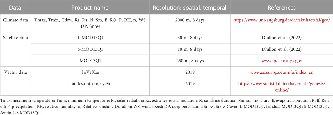
TABLE 1. Summary of collected datasets for winter wheat (WW) and oil seed rape (OSR) crop modeling.
2.1.1 Satellite data
The present study used two synthetic [L-MOD13Q1 (30 m, 8-days) and S-MOD13Q1 (10 m, 8-days)] and one real-time [MOD13Q1 (250 m, 8-days)] NDVI time series, which were generated in preceding work by (Dhillon et al., 2022)] as an input to the RF and LUE models. In the synthetic NDVI products, the cloud and shadow gaps in the real-time Sentinel-2 and Landsat data for 2019 were filled using the spatial and temporal adaptive reflectance fusion model (STARFM), which blends the coarse spatial resolution of MODIS and high spatial resolution of Landsat/Sentinel-2 data. In addition, the MOD13Q1 V6 product (just the MODIS NDVI time series without image fusion) is also selected as an input to the RF and LUE models to allow the comparison of crop yield outputs at high (10 m), medium (30 m) and coarse (250 m) spatial scales. The 8-day time series for the RS products are considered starting at the day of the year (DOY) 1 (1 January) till 353 (19 December) for 2019. For crop modelling and machine learning algorithms, this study inputs the 8-day satellite datasets from the stem elongation phases till the flowering stages of both WW and OSR. For OSR, the SOS is 15th February, and the EOS is 20th April 2019 (Zamani-Noor and Feistkorn, 2022). And for WW, the SOS and EOS period lies between 15th of April to 30th of June 2019 (Harfenmeister et al., 2021).
2.1.2 Climate data
For input to the RF and LUE models, the climate data for 2019 with daily temporal resolution includes 80 variables considering the sum, mean, maximum, minimum, and standard deviation (sd) for each variable during the time frame. The climate variables included are maximum (T_max, oC), minimum (T_min, oC) and dew point (T_dew, oC) temperature, solar radiation (Rs, MJm−2day−1), sunshine hours (N, hours), relative sunshine duration (n, hours), precipitation (P, mm), soil moisture (Sm, mm), relative humidity (RH, %), wind speed at 2 m height (WS, ms−1), runoff (RO, mm), deep percolation (DP, mm), snow cover (Snow, mm), extra-terrestrial radiation (Ra, MJm−2day−1), Sublimation (Sublim, mm) and evapotranspiration (E, mm). The CV were obtained by dynamical downscaling the ERA5 reanalysis dataset (Hersbach et al., 2020), provided by the European Centre for Medium-Range Weather Forecasts, to a horizontal grid resolution of 2000 m using the hydrologically enhanced Weather Research and Forecasting model (Gochis et al., 2018; Skamarock et al., 2019). A detailed description of the selected downscaling approach is provided by (Arnault et al., 2018) and (Rummler et al., 2019). For this research, the daily climate data is aggregated into 8 days’ temporal products and adapted to the RF and LUE models. Like the satellite data, the present study considers the 8-day climate data for the same SOS and EOS for WW and OSR as described in Section 2.1.1.
2.1.3 InVeKos data
The InVeKos data is field-based data used to identify the fields of WW and OSR in 2019. The data is collected through the Integrated Administration Control Systems (IACS) (www.etc.europa.eu/info/index_en) that is available for all agricultural plots in the European Union (EU) countries by allowing farmers to graphically indicate their agricultural areas. In the IACS, EU countries are responsible for administering and controlling payments to farmers through a principle called shared management.
2.1.4 Bayerisches Landesamt für statistik (LfStat) crop yield data
The LfStat crop yield is a database that provides crop yield of 29 crop categories including WW and OSR in Bavaria at a regional level (source: https://www.statistikdaten.bayern.de/genesis/online/, Statistics Code: 41241). In this study, LfStat crop yield data of WW [total number of observations (n = 65 and OSR n = 50)] is used for training (70%) and testing (30%) the RF models and for validating the LUE model (100%), respectively (see Figure 1).
2.2 Method
2.2.1 LUE model
The study used the semi-empiric LUE model based on the principle of light use efficiency theory (Monteith, 1972; Monteith, 1977). As it is proven to be reliable, precise, and accurate, this study used the same approach to calculate crop yield and biomass as adopted by (Dhillon et al., 2020). The model monitors the growth of WW and OSR by assessing the impact of climate variables over a period of 8 days between their respective SOS and EOS and calculates the crop biomass as a cumulative sum. The climate variables used by the LUE model are (CV2) T_mean, T_max, T_dew, Rs, and RH. The model is based on a semi-empirical approach and calculates the aboveground biomass as a cumulative sum between the stem elongation phase till the flowering stage of both WW and OSR (Eq. 1),
where PAR is photosynthetically active radiation (MJ m−2 d−1), FPAR is the fraction of PAR absorbed by the canopy, є is the actual light-use efficiency (g C M J−1) and i is the time frame between the SOS (stem elongation) and the EOS (flowering period) of both crops. The total aboveground biomass calculated by the LUE model is equivalent to the net primary productivity (NPP) (kg ha−1 yr−1) (Monteith, 1972; Gitelson et al., 2012). The detailed stepwise procedure of the LUE model is explained in (Dhillon et al., 2020).
2.2.2 Random forest (RF) model
The study trained and used four RF models (RF1, RF2, RF3, and RF4) (see Figure 1), binary-bias machine-learning methods, to predict crop yields for WW and OSR. RF can be used for classification and regression purposes and this study used it as a regression tool. The RF model is trained by many classification and regression trees (CARTs) that are grown with a random subset of predictors Many random trees are generated when the source data for the model is bootstrapped and, finally, the forest (group of random trees) of the CART is averaged. A more detailed explanation of the model is provided by (Breiman, 2001). The study used the ‘randomForest’ package in the software R for each RF model (Liaw and Wiener, 2002; Team, 2013) (Table 2). The value of mtry has been approximately considered by dividing the total number of predictors by 3. A variable analysis tool from the randomForest package analyses the variable importance. The mean decrease accuracy is used as a measure of variable importance. The out-of-bag (OOB) performance estimation is analyzed for assessing the performance by averaging the node’s mean decrease accuracy before and after permuted.
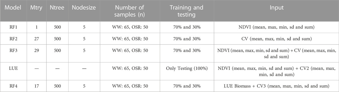
TABLE 2. Input requirements of different Random Forest (RF) models (RF1, RF2, RF3, and RF4) implemented using the package ‘randomForest’ in the software R. CV represents to climate variables.
2.2.3 Statistical analysis
The modeled crop yield data from four RF and LUE models are validated with the Landesamt district-wise yield data collected from the statistics department of Bavaria for the year 2019. From the modeled and referenced yield, the determination coefficient (R2) (Eq. 2), mean error (ME), root mean square error (RMSE), and relative RMSE (RRMSE) (Eqs 3, 4, 5) are calculated. The lower the value of ME, RMSE and RRMSE the better the model performed. This study considers RRMSE <15% as good agreement; 15–30% as moderate agreement; and >30% as poor agreement (Yang et al., 2014). A linear regression model (LRM) is performed to establish a linear relationship between the referenced and modeled yield of WW and OSR at different spatial scales (10, 30, and 250 m).
where Pi is the predicted value, Oi is the observed value, Ō is the observed mean value, and n is the total number of observations. The significance of the used models is checked by analyzing the probability value (p-value), which is calculated using the LRM with a H0 that there is no correlation between the referenced and modeled yield, and an H1 that the relationship exists. To perform this test, a significance level (called alpha (α)) is set to 0.05. A p-value of less than 0.05 shows that a model is significant, and it rejects the H0 that there is no relationship.
3 Results
3.1 RF1: NDVI as the only predictor of crop yield monitoring
With L-MOD13Q1, S-MOD13Q1, and MOD13Q1 NDVI inputs, the RF1 model performed significantly for WW and OSR (p-value <0.05). The R2 obtained from the S-MOD13Q1 NDVI product has a higher accuracy than the L-MOD13Q1 and MOD13Q1 (Figure 3). Based on the R2 of different spatial resolutions of the NDVI products for WW and OSR, the RF models resulted in descending order as S-MOD13Q1 (10 m), L-MOD13Q1 (30 m), and MOD13Q1 (250 m), with R2 values as 0.66/0.61, 0.66/0.50, and 0.60/0.26, respectively. For quality and precision, the ME and RMSE values give a more complete picture of the performance of RF with NDVI as the only predictor. The ME and RMSE of WW from MOD13Q1 (8.21 dt/ha and10.30 dt/ha) are higher than that of L-MOD13Q1 (8.18 dt/ha and 10.20 dt/ha) and S-MOD13Q1 (5.65 dt/ha and 7.96 dt/ha), respectively (Figures 3A,C,E). Similarly, for OSR, S-MOD13Q1 has the lowest ME and RMSE of 2.76 dt/ha and 3.76 dt/ha, as compared to L-MOD13Q1 and MOD13Q1 (Figures 3B,D,F). Overall, the S-MOD13Q1 (RRMSE = 11.40% (WW)/11.23% (OSR)) results are more accurate than L-MOD13Q1 (14.33%/12.28%) and MOD13Q1 (14.83%/14.32%) for both WW and OSR.
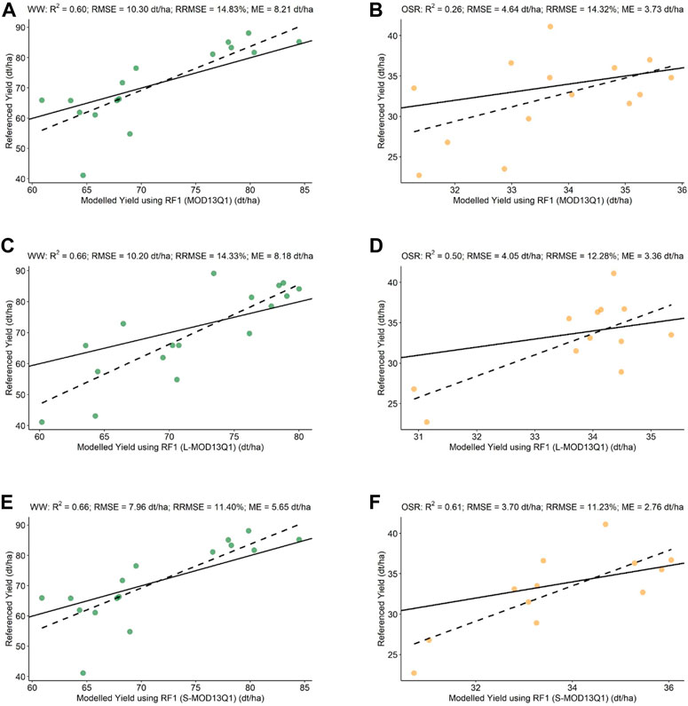
FIGURE 3. Scatter plots of the validation of WW and OSR modeled yield using RF1 model with referenced yield. The green dots represent WW, and the orange dots represent OSR. (A) MOD13Q1 (RF1(WW); just MODIS) versus referenced yield. (B) MOD13Q1 (RF1(OSR); just MODIS) versus referenced yield. (C) L-MOD13Q1 (RF1(WW); Landsat and MODIS) versus referenced yield. (D) L-MOD13Q1 (RF1(OSR); Landsat and MODIS) versus referenced yield. (E) S-MOD13Q1 (RF1(WW); Sentinel-2 and MODIS) versus referenced yield. (F) S-MOD13Q1 (RF1(OSR); Sentinel-2 and MODIS) versus referenced yield. Every plot contains a solid 1:1 line that is used to visualize the correlation between referenced and synthetic yield.
3.2 RF2: Climate variables (CV) as the only predictors of crop yield monitoring
With climate elements as input parameters, the RF2 model performed significantly for both WW and OSR (p-value <0.05) (Figures 4A,B). The R2 obtained for WW has shown a higher accuracy (R2 = 0.57) than the OSR (R2 = 0.50). However, the OSR (RMSE = 4.23 dt/ha) resulted in higher preciseness than the WW (RMSE = 10.60 dt/ha). Moreover, the RRMSE for WW shows moderate agreement (15.28%) between the observed and predicted yield. The CV importance for WW are mainly N, E, Ra, Tdew, Sm, and Rs; however, for OSR, Tmin, WS, Ra, Rs, and Snow are of high importance (Figures 4C,D).
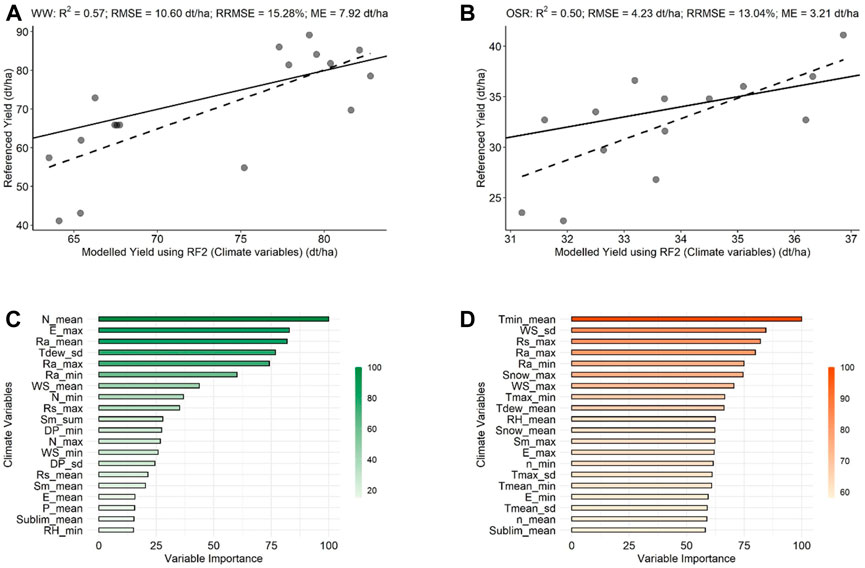
FIGURE 4. Scatter and bar plots of the validation of WW and OSR modeled yield with referenced yield and the variable importance using the RF2 model, respectively. The green color represents WW, and the orange color represents OSR. (A) RF2 [WW using climate variables (CV)] versus referenced yield. (B) RF2 [OSR using climate variables (CV)] versus referenced yield. (C) Variable importance for WW (D) Variable importance for OSR.
3.3 RF3: NDVI and CV predictors for crop monitoring
With climate parameters and L-MOD13Q1, S-MOD13Q1, and MOD13Q1 NDVI inputs, the RF3 model performed significantly for WW and OSR (p-value <0.05). The R2 obtained from the S-MOD13Q1 NDVI product has a higher accuracy than the L-MOD13Q1 and MOD13Q1 (Figure 5). Based on the R2 of different spatial resolutions of the NDVI products for WW and OSR, the RF models resulted in descending order as S-MOD13Q1 (10 m), L-MOD13Q1 (30 m), and MOD13Q1 (250 m), with R2 values of 0.75 (WW)/0.66(OSR), 0.72/0.61, and 0.67/0.53, respectively. For quality and precision, the ME and RMSE values give a more complete picture of the performance of RF with NDVI as the only predictor. The ME and RMSE of WW from MOD13Q1 (5.56 dt/ha and 8.10 dt/ha) are higher than that of L-MOD13Q1 (5.45 dt/ha and 7.98 dt/ha) and S-MOD13Q1 (4.94 dt/ha and 7.56 dt/ha), respectively (Figures 5A,C,E). Similarly, for OSR, S-MOD13Q1 has the lowest ME and RMSE of 2.70 dt/ha and 3.78 dt/ha, as compared to L-MOD13Q1 (2.77 dt/ha and 3.85 dt/ha) and MOD13Q1 (3.11 dt/ha and 4.08 dt/ha) (Figures 5B,D,F). The RRMSE is decreased by −6.57% and −7.23% between S-MOD13Q1 (10.66% (WW) and 11.67% (OSR)) and MOD13Q1 (11.41% and 12.58%) for WW and OSR, respectively. The mean and sum of NDVI have a higher impact on the accuracy assessment of WW yield; however, NDVI has less impact on the crop yield prediction of OSR (Figure 6). Other than that, E, Ra, Sm, and N have a higher influence on WW’s yield prediction (Figure 6A). For OSR, Snow, Temperature, and Sm have shown a higher influence (Figure 6B).

FIGURE 5. Scatter plots of the validation of WW and OSR modeled yield using RF3 model with referenced yield. The green dots represent WW, and the orange dots represent OSR. (A) MOD13Q1 [RF3(WW); just MODIS] versus referenced yield. (B) MOD13Q1 [RF3(OSR); just MODIS] versus referenced yield. (C) L-MOD13Q1 (RF3(WW); Landsat and MODIS) versus referenced yield. (D) L-MOD13Q1 [RF3(OSR); Landsat and MODIS] versus referenced yield. (E) S-MOD13Q1 [RF3(WW); Sentinel-2 and MODIS] versus referenced yield. (F) S-MOD13Q1 [RF3(OSR); Sentinel-2 and MODIS] versus referenced yield. Every plot contains a solid 1:1 line that is used to visualize the correlation between referenced and synthetic yield.

FIGURE 6. Bar plots of the variable importance of WW and OSR after validation of the modeled yield with referenced yield using the RF3 model. The green color represents WW, and the orange color represents OSR. (A) Variable importance for WW (B) Variable importance for OSR.
3.4 Light use efficiency (LUE) model
With the different spatial outputs, the LUE model performed significantly for WW and OSR (p-value <0.05) (Figure 7). For WW, the S-MOD13Q1 (R2 = 0.86, RMSE = 5.03 dt/ha, RRMSE = 7.36%) has higher accuracy and preciseness than the L-MOD13Q1 (R2 = 0.83, RMSE = 5.64 dt/ha, RRMSE = 9.76%) and MOD13Q1 (R2 = 0.65, RMSE = 7.63 dt/ha, RRMSE = 9.84%) (Figures 7A,C,E). Similarly, for OSR, the LUE model ordered as S-MOD13Q1, L-MOD13Q1, and MOD13Q1, with high R2 and low RMSE and RRMSE values as 0.82/2.14 dt/ha/9.12%, 0.80/2.17 dt/ha/9.46%, and 0.66/3.12 dt/ha/10.51%, respectively (Figures 7B,D,F).
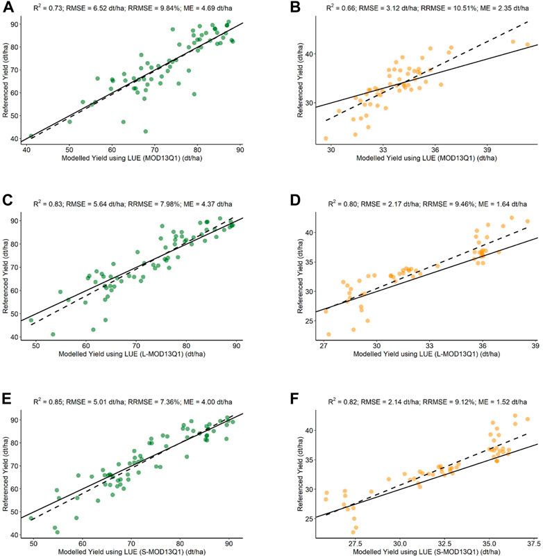
FIGURE 7. Scatter plots of the validation of WW and OSR modeled yield using LUE model with referenced yield. The green dots represent WW, and the orange dots represent OSR. (A) MOD13Q1 (LUE (WW); just MODIS) versus referenced yield. (B) MOD13Q1 [LUE (OSR); just MODIS] versus referenced yield. (C) L-MOD13Q1 [LUE (WW); Landsat and MODIS] versus referenced yield. (D) L-MOD13Q1 (LUE (OSR); Landsat and MODIS) versus referenced yield. (E) S-MOD13Q1 [LUE (WW); Sentinel-2 and MODIS] versus referenced yield. (F) S-MOD13Q1 [LUE (OSR); Sentinel-2 and MODIS] versus referenced yield. Every plot contains a solid 1:1 line that is used to visualize the correlation between referenced and synthetic yield. The validation of LUE model is performed for a total number of samples for both WW and OSR which increases the number of points in the scatter plot.
3.5 RF4: Coupling LUE and RF for crop yield prediction
On linking the LUE model outputs with climate parameters (CV3), the S-MOD13Q1 (R2 = 0.91, RMSE = 4.98 dt/ha, RRMSE = 7.29%) has higher accuracy and preciseness than the L-MOD13Q1 (R2 = 0.88, RMSE = 5.63 dt/ha, RRMSE = 7.93%) and MOD13Q1 (R2 = 0.77, RMSE = 6.80 dt/ha, RRMSE = 9.58%) for WW (Figures 8A,C,E). Similarly, for OSR, the RF4 model ordered as S-MOD13Q1, L-MOD13Q1, and MOD13Q1, with high R2 and low RMSE and RRMSE values as 0.84/2.11 dt/ha/8.83%, 0.84/2.16 dt/ha/9.42%, and 0.74/3.11 dt/ha/10.37%, respectively (Figures 8B,D,F). For both WW and OSR, the biomass output of the LUE model has shown the highest impact in improving the accuracy of the respective crop yields (Figure 9).
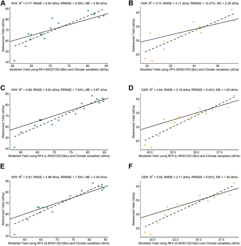
FIGURE 8. Scatter plots of the validation of WW and OSR modeled yield using RF4 model with referenced yield. The green dots represent WW, and the orange dots represent OSR. (A) MOD13Q1 [RF4(WW); just MODIS] versus referenced yield. (B) MOD13Q1 (RF4(OSR); just MODIS) versus referenced yield. (C) L-MOD13Q1 [RF4(WW); Landsat and MODIS] versus referenced yield. (D) L-MOD13Q1 (RF4(OSR); Landsat and MODIS) versus referenced yield. (E) S-MOD13Q1 [RF4(WW); Sentinel-2 and MODIS] versus referenced yield. (F) S-MOD13Q1 [RF4(OSR); Sentinel-2 and MODIS] versus referenced yield. Every plot contains a solid 1:1 line that is used to visualize the correlation between referenced and synthetic yield.

FIGURE 9. Bar plots of the variable importance of WW and OSR after validation of the modeled yield with referenced yield using the RF4 model. The green color represents WW, and the orange color represents OSR. (A) Variable importance for WW (B) Variable importance for OSR.
3.6 Overall comparison of models
The bar plots in Figure 10 show the accuracy assessment of estimating crop yields of WW and OSR using different models with different inputs. For the model RF1 (where NDVI is the only predictor), the MOD13Q1 has the lowest R2 [0.60 (WW)/0.26 (OSR)] while both L-MOD13Q1 and S-MOD13Q1 have almost the same R2 values (0.66/0.50) for both WW and OSR. However, for WW, the RMSE and RRMSE has shown a different trend with lower values (7.96 dt/ha, 11.40%) for S-MOD13Q1, and higher (10.22 dt/ha, >14.00%) for both MOD13Q1 and L-MOD13Q1. The RF2 model (where climate variables are predictors), has shown the lowest accuracy [R2: 0.57 (WW), 0.50 (OSR)] and preciseness (RMSE: 10.6 dt/ha, 4.23 dt/ha) as compared to the RF1 model. The RF3 model (where CV and NDVI are the predictors), has improved the accuracy estimation of RF1 with higher R2 (CV + S-MOD13Q1> CV + L-MOD13Q1> CV + MOD13Q1) and lower RMSE and RRMSE (CV + S-MOD13Q1< CV + L-MOD13Q1< CV + MOD13Q1) for both WW and OSR. On the other hand, the LUE model has further improved the R2 and RMSE values for both crops than the RF3 model. The accuracy of the LUE model is in descending order from CV2+S-MOD13Q1, CV2+L-MOD13Q1, and CV2+MOD13Q1. The CV2 are the climate variables inputted by the LUE model. Lastly the RF4 model [which combines the biomass output of LUE with additional CV3(CV minus CV2)], S-MOD13Q1 provided the highest accuracy [0.91 (WW)/0.84 (OSR)] and lower RRMSE (7.29%/8.83%) for both WW and OSR among the investigated models. The coupling of the LUE model variables to the RF4 model can decrease the RMSE by −1.00% (for WW) and −8.4% (for OSR), decrease the RRMSE from −8% (WW) and −1.6% (OSR), and increase the R2 by 14.3% (for both WW and OSR), compared to results just relying on LUE. Similarly, between RF1 and RF4, the RRMSE has been decreased by −36.05% (WW) and −21.37% (OSR).
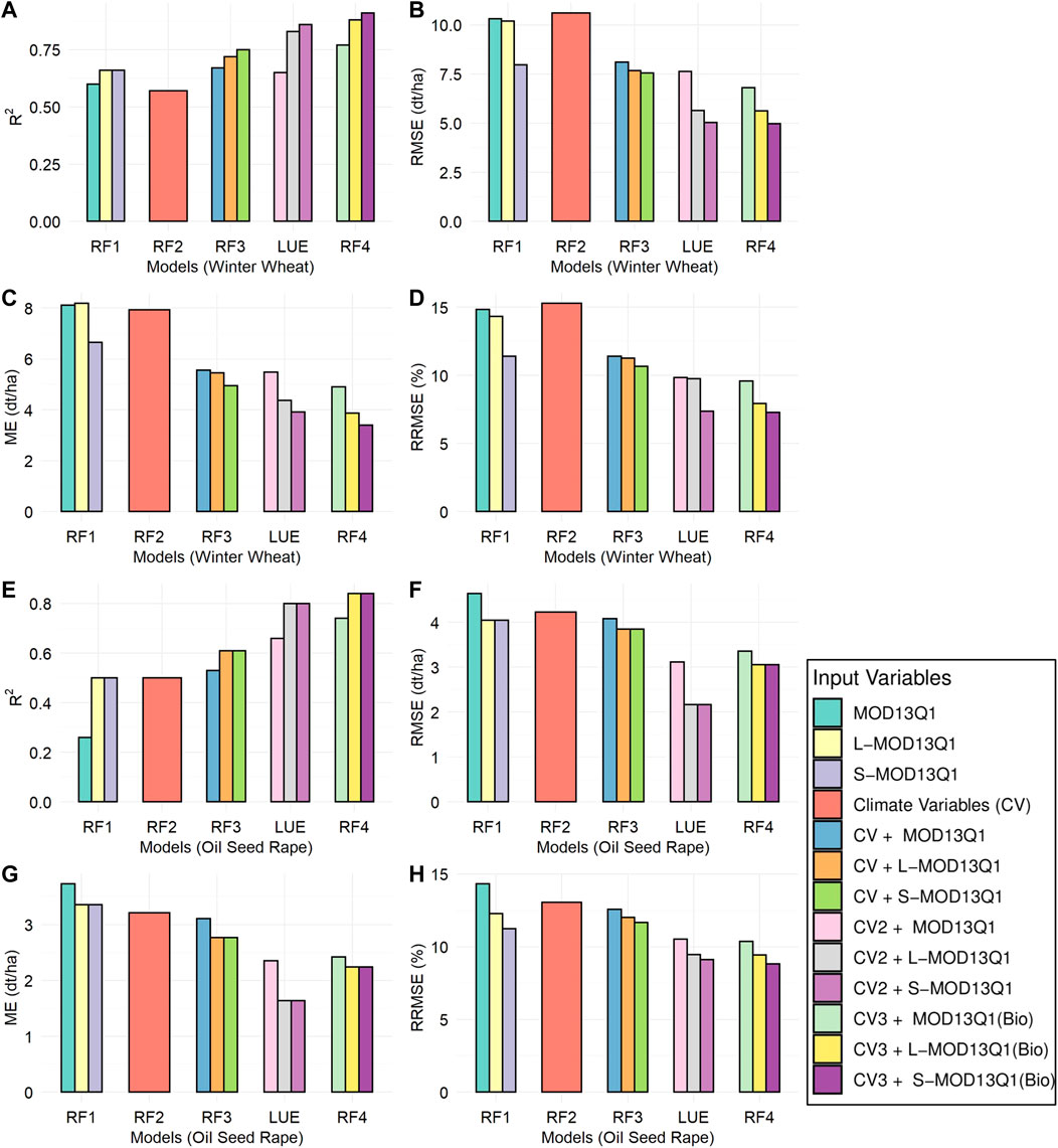
FIGURE 10. Bar plots for the overall accuracy assessment of WW and OSR with four RF (RF1, RF2, RF3, RF4) and one LUE model with different input variables (shown in the legend at right). (A) R2, (B) RMSE, (C) ME, and (D) RRMSE for WW and (E) R2, (F) RMSE, (G) ME, and (H) RRMSE for OSR using different models with various inputs, respectively.
3.7 Accuracy assessment based on different spatial inputs
The box plots in Figure 11 show the contribution of different spatial inputs to LUE and RF models crop yield estimations of Bavaria for WW and OSR. Among all models, the S-MOD13Q1 (10 m) result in higher mean R2 [0.80 (WW)/0.69 (OSR)], lower RMSE (dt/ha) (6.38/3.05), lower RRMSE (%) (9.18, 10.21) compared to L-MOD13Q1 (30 m) and MOD13Q1 (250 m). For WW, both S-MOD13Q1 and L-MOD13Q1 resulted in similar accuracy; however, for OSR, S-MOD13Q1 performed better than L-MOD13Q1. Moreover, the MOD13Q1 resulted in better performance for OSR than WW. For L-MOD13Q1 and MOD13Q1, the mean R2 (0.77 (WW)/0.69 (OSR), 0.67/0.55), RMSE (dt/ha) (7.29/3.06, 8.21/3.74) and RRMSE (%) (10.82/10.79, 11.42/11.95) values vary in an order of higher accuracy.
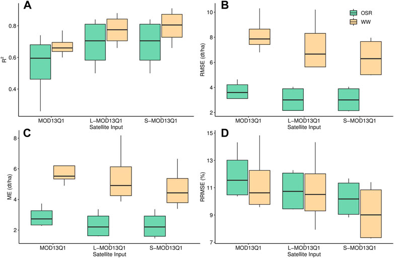
FIGURE 11. Box plots show the comparison of the accuracy assessment of three satellite inputs (S-MOD13Q1 (10 m), L-MOD13Q1 (30 m) and MOD13Q1 (250 m)) used in four models (RF1, RF3, LUE, and RF4) for yield prediction of WW and OSR. (A) R2 (B) RMSE (C) ME and (D) RRMSE.
3.8 Spatial distribution of crop yields for WW and OSR on regional scale
The maps in Figures 12, 13 describe the region-wise spatial distribution of referenced and predicted (obtained from RF1, RF2, RF3, LUE and RF4) yield for WW and OSR by inputting S-MOD13Q1 (10 m) in Bavaria for the year of 2019, respectively. For both crops, the yield prediction by the RF4 (coupling of LUE and RF) has better synchronization with the observed yield results compared to the other four models. The referenced OSR and WW yields have higher values in the southern regions of Bavaria. Almost all models for OSR have shown higher values in respective regions; however, for WW, only RF4 and LUE modelled yields obtained higher values (>85 dt/ha) and other models have estimated between 55 and 85 dt/ha. The referenced OSR yield values for the central part of Bavaria observed higher yield between 32 and 44 dt/ha; however only RF4 and RF3 models had predicted the accurate amount.
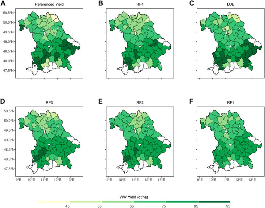
FIGURE 12. Spatial distribution of referenced yield and predicted yield for WW using RF1, RF2, RF3, LUE and RF4 models by inputting S-MOD13Q1 (10 m) for the state of Bavaria in 2019. The white color represents no data available. (A) Referenced Yield (B) RF4 (C) LUE, (D) RF3, (E) RF2, and (F) RF1.
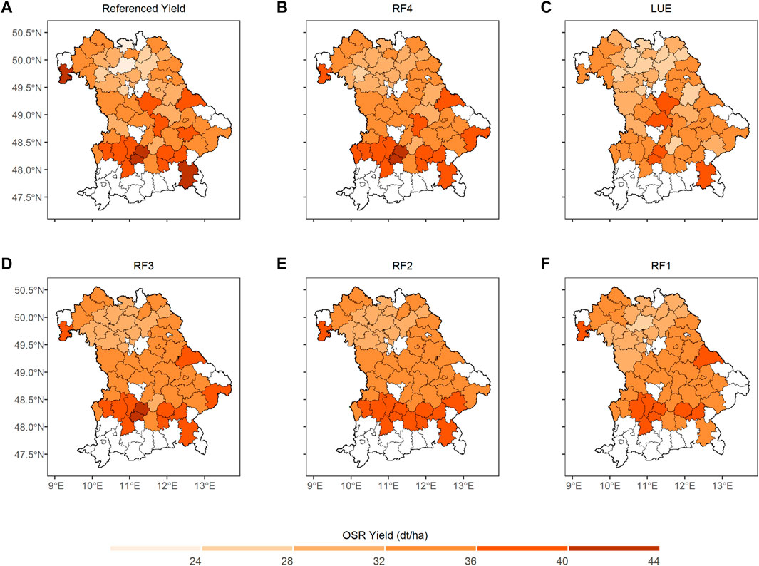
FIGURE 13. Spatial distribution of referenced yield and predicted yield for OSR using RF1, RF2, RF3, LUE and RF4 models by inputting S-MOD13Q1 (10 m) for the state of Bavaria in 2019. The white color represents no data available. (A) Referenced Yield (B) RF4 (C) LUE, (D) RF3, (E) RF2, and (F) RF1.
4 Discussion
This study addresses the importance of coupling the RF model with the LUE model to improve the accuracy of crop yield estimation of WW and OSR for Bavaria in 2019. The present study is among the rare other studies that ensemble models to increase crop yield predictability. This study demonstrated that introducing the LUE output spatial biomass plus climate parameters into the RF model (RF4) and utilizing them as inputs to a prediction task on average can decrease the prediction error measure by RMSE from 5.03–4.98 dt/ha (for WW) and 2.14–1.96 dt/ha (for OSR). In addition, the predictions made by the RF4 model show less bias towards the actual regional yields. Similar studies in this area are only limited to coupling the simplest statistical models with crop growth models (Chakraborty et al., 2005; Hadria et al., 2006; De Wit and Van Diepen, 2007; Dente et al., 2008). However, a related study has coupled the Agricultural Production Systems Simulator (APSIM) variables into machine learning models and estimated the decrease of RMSE between 7 and 20% (Shahhosseini et al., 2021).
The cloud and shadow gaps in the optical satellite data can hinder or limit yield prediction algorithms from producing accurate yield results (Roy et al., 2008; Gevaert and García-Haro, 2015). Many studies employing satellite images aimed to compensate the data gaps present in satellite data by fusing it with another data source for various applications of remote sensing (Barbedo, 2022). The research is conducted at different spatial scales where multiple spatial resolution satellite products [two STARFM-derived synthetic NDVI products (L-MOD13Q1 (30 m, 8 days) and S-MOD13Q1 (10 m, 8 days and one real NDVI product (MOD13Q1 (250 m, days)] are inputted to different RF models (Dhillon et al., 2022). The study highlights the importance of high spatial scales in achieving accurate crop yield results. For example, the input products with 10-m resolutions (R2 > 0.75) resulted in higher accuracy than the 30-m (R2 > 0.72) and 250-m (R2 > 0.65) satellite products using RF2, RF3, and RF4 models for WW. Previous studies have also shown that high spatial resolution could significantly improve the accuracy of crop yields (Huang et al., 2016; Dhillon et al., 2020; LIU et al., 2021).
Moreover, the results of the study at hand also demonstrate that variable selection plays an important role in achieving more accurate crop predictions. The time series vegetation index (VI) data derived from satellite images are known as a better predictor for many applications of remote sensing (Zhang et al., 2003; Wardlow et al., 2007; Zhong et al., 2012; Zhang et al., 2013; Kim et al., 2014; Shen et al., 2015); however, this study highlights that NDVI alone could not be used to achieve accurate crop yield results (WW: R2 < 0.65, OSR: R2 < 0.45). Moreover, the research found that the combined use of NDVI and climate parameters can help to improve the model performance (WW: R2 > 0.70, OSR: R2 > 0.60). The inclusion of relevant climate parameters positively impacted the yield prediction for WW and OSR. For example, extra-terrestrial radiation has higher variable importance for WW and snow cover for OSR. Furthermore, the crop and phenology-related variables (LUE biomass), solar radiation, soil moisture and temperature are the most influential variables in increasing the yield accuracy for WW and OSR.
This study also compares the performance of LUE when used with and without the random forest model. Similar to other studies, the LUE model resulted precisely and accurately with an average R2 of 0.78 and 0.76 and an RMSE of 6.10 and 2.47 dt/ha for WW and OSR at different spatial scales, respectively (Dhillon et al., 2020). However, a drastic improvement in the accuracy has been seen when the LUE model was linked with the random forest model by including more climate variables as an input. This coupling has increased the R2 from 0.78 to 0.85 and 0.76 to 0.81 for WW and OSR using different satellite inputs, respectively.
The simplicity and reliability of the present study conclude that this design needs to be implemented for different periods, locations, and crop types to improve the global yield estimation for developing agricultural policies, improving food security, forecasting, and analyzing global trade trends. The study stresses coupling the LUE model with the RF model; however, the applicability of other crop models, such as WOFOST, AquaCrop, or CERES Wheat, on coupling with ML or deep learning (DL) could be tested. Moreover, the study only includes the year 2019 for the state of Bavaria, but the same design could be transferred and tested to other geographical regions at any time scale. Inclusion of climatic variables such as solar radiation, extra-terrestrial radiation, soil moisture, temperature, snow cover (for OSR) and evapotranspiration would be recommended in future studies. Due to the availability of the crop validation data (LfStat) on a regional level, the study integrated the pixel-level information into the district level. This transfer of data (from field to district level) could result in a loss of information, and it might negatively impact the accuracy of the algorithm outcomes. Therefore, to justify the potential of satellite data and machine learning algorithms in crop monitoring, the study recommends testing and validating methodology at the field level. Moreover, as the study validates the accuracy of WW and OSR, the study design might also be tested for different crop types such as Maize, Sugarcane, Rice, etc.
5 Conclusion
Conclusively, this study stressed the positive impact of combining crop modeling and machine learning to improve the prediction accuracies for the application of agricultural monitoring. Moreover, the crop and phenology-related inputs (LUE biomass), extra-terrestrial radiation, solar radiation, evapotranspiration, extra-terrestrial radiation, soil moisture, snow cover (for OSR) and temperature are the most influential variables that are needed to be considered for increasing the yield accuracy in future studies. The present research concludes the findings as follows:
(i) To answer if NDVI or CV is the better predictors of crop yield, the study found that the individual use of NDVI (in RF1) and climate variables (in RF2) would be less accurate in yield prediction than they are used together (in RF3) in machine learning. The accuracy assessment when NDVI is used alone as a crop yield predictor is lower (WW: R2 < 0.65, OSR: R2 < 0.45) than it is used together with the climate variables (WW: R2 > 0.70, OSR: R2 > 0.60).
(ii) To find if the coupling of ML and CGM results in higher accuracy, the study investigated that linking the LUE model’s output with the RF model’s input (RF4) would increase the crop yields’ accuracy drastically. The coupling has decreased the RMSE by -1.00% (for WW) and -8.4% (for OSR), decreased the RRMSE from -8% (WW) and -1.6% (OSR), and increased the R2 by 14.3% (for both WW and OSR), compared to results of LUE.
(iii) To find the impact of high spatial resolution on crop yield estimation, the study concludes that the RS inputs with 10-m resolutions resulted in higher accuracy than the 30-m and 250-m with RF2, RF3, LUE, and RF4 models for WW and OSR.
Moreover, the present study is performed at the regional level; however, the availability of field-level yield information could be useful for implementing a similar methodology and obtaining more accurate outcomes. The study design needs to be implemented for different periods, locations, and crop types to improve the global yield estimation for developing agricultural policies, improving food security, forecasting, and analyzing global trade trends. The accurate validations of WW and OSR broaden the scope of the study. Therefore, the simple and reliable design of the study could be tested for other crop types such as maize, sugarcane, or rice on a global scale.
Data availability statement
The original contributions presented in the study are included in the article/supplementary material, further inquiries can be directed to the corresponding author.
Author contributions
MD wrote the first draft of the manuscript. MD and TU contributed to editing. MD and TU contributed to the analysis. MD and TU contributed to conceptualization. MD contributed to methodology. MD and TU contributed to formal analysis. TU contributed to supervision. MS-D, C-KF, TR, and JA contributed to data curation. MD, TD, CK-F, TR, JA, IS-D, and TU contributed to resources. MD, CK-F, and TD contributed to project administration. TU and IS-D contributed to funding acquisition.
Funding
This study was conducted within the LandKlif project funded by the Bavarian Ministry of Science and the Arts via the Bavarian Climate Research Network (bayklif, www.bayklif.de). This publication was supported by the Open Access Publication Fund of the University of Wuerzburg.
Acknowledgments
The authors thankfully express gratitude to the National Aeronautics and Space Administration (NASA) Land Processed Distributed Active Archive Center (LP DAAC) for MODIS; U.S. Geological Survey (USGS) Earth Resources Observation and Science (EROS) Center for Landsat; The Copernicus Sentinel-2 mission for the Sentinel-2 data; The Bavarian State Office for Statistics (Landesamt) for providing the crop yield data for Winter wheat and Oil Seed Rape; Professorship of Ecological Services, University of Bayreuth, for the updated InVeKos data 2019; Jie Zhang and Sarah Redlich, both Department of Animal Ecology and Tropical Biology, University of Wuerzburg; together with Melissa Versluis, Rebekka Riebl, Maria Hänsel, Bhumika Uniyal, Thomas Koellner (all Professorship of Ecological Services, University of Bayreuth); we acknowledge the data providers for the base layer IACS (Bayerisches Staatsministerium für Ernährung, Landwirtschaft und Forsten); we are also thankful to Marlene Bauer and Annemarie Lass for initiating this wonderful work in their innovation project; University of Augsburg for providing the Climate Data for this study; Simon Sebold for providing all technical and computational help during the complete fusion processing of Landsat/Sentinel-2 and MODIS; Department of Remote Sensing, University of Wuerzburg, for providing all necessary resources and support; Google Earth Engine platform for faster downloading and preprocessing the large data sets of Bavaria; The Comprehensive R Archive Network (CRAN) for running the STARFM, and validating and visualizing the data outputs using R packages such as raster, rgdal, ggplot2, ggtools, randomForest and xlsx; ArcGIS 10.8 and ArcGIS pro 2.2.0 maintained by Environmental Systems Research Institute (Esri) for generating maps and Bavarian Land Cover Map of 2019; and the Bavarian Ministry for Science and the Arts via the Bavarian Climate Research Network (bayklif) for funding.
Conflict of interest
The authors declare that the research was conducted in the absence of any commercial or financial relationships that could be construed as a potential conflict of interest.
Publisher’s note
All claims expressed in this article are solely those of the authors and do not necessarily represent those of their affiliated organizations, or those of the publisher, the editors and the reviewers. Any product that may be evaluated in this article, or claim that may be made by its manufacturer, is not guaranteed or endorsed by the publisher.
Abbreviations
CGMs, crop growth models; CV, climate variable; DOY, day of the year; L-MOD13Q1, Landsat-MOD13Q1; LUE, light use efficiency; ME, mean error; ML, machine learning; MODIS, moderate resolution imaging spectroradiometer; NDVI, normalized difference vegetation index; OSR, oil seed rape; RF, random forest; RRMSE, relative root mean square error; RS, remote sensing; S-MOD13Q1, Sentinel-2-MOD13Q1; STARFM, spatial and temporal adaptive reflectance fusion model; WW, winter wheat.
References
Ali, A. M., Abouelghar, M. A., Belal, A.-A., Saleh, N., Younes, M., Selim, A., et al. (2022). Crop yield prediction using multi sensors remote sensing (review article). Egypt. J. Remote Sens. Space Sci. 25, 711–716. doi:10.1016/j.ejrs.2022.04.006
Archontoulis, S. V., Castellano, M. J., Licht, M. A., Nichols, V., Baum, M., Huber, I., et al. (2020). Predicting crop yields and soil-plant nitrogen dynamics in the US Corn Belt. Crop Sci. 60 (2), 721–738. doi:10.1002/csc2.20039
Arnault, J., Rummler, T., Baur, F., Lerch, S., Wagner, S., Fersch, B., et al. (2018). Precipitation sensitivity to the uncertainty of terrestrial water flow in WRF-Hydro: An ensemble analysis for central Europe. J. Hydrometeorol. 19 (6), 1007–1025. doi:10.1175/jhm-d-17-0042.1
Barbedo, J. G. A. (2022). Data fusion in agriculture: Resolving ambiguities and closing data gaps. Sensors 22 (6), 2285. doi:10.3390/s22062285
Basso, B., and Liu, L. (2019). Seasonal crop yield forecast: Methods, applications, and accuracies. Adv. Agron. 154, 201–255. doi:10.1016/bs.agron.2018.11.002
Benabdelouahab, T., Lebrini, Y., Boudhar, A., Hadria, R., Htitiou, A., and Lionboui, H. (2019). Monitoring spatial variability and trends of wheat grain yield over the main cereal regions in Morocco: A remote-based tool for planning and adjusting policies. Geocarto Int. 36, 2303–2322. doi:10.1080/10106049.2019.1695960
Bhandari, S., Phinn, S., and Gill, T. (2012). Preparing landsat image time series (LITS) for monitoring changes in vegetation phenology in queensland, Australia. Remote Sens. 4 (6), 1856–1886. doi:10.3390/rs4061856
Bogard, M., Biddulph, B., Zheng, B., Hayden, M., Kuchel, H., Mullan, D., et al. (2020). Linking genetic maps and simulation to optimize breeding for wheat flowering time in current and future climates. Crop Sci. 60 (2), 678–699. doi:10.1002/csc2.20113
Chakraborty, M., Manjunath, K., Panigrahy, S., Kundu, N., and Parihar, J. (2005). Rice crop parameter retrieval using multi-temporal, multi-incidence angle Radarsat SAR data. ISPRS J. Photogrammetry Remote Sens. 59 (5), 310–322. doi:10.1016/j.isprsjprs.2005.05.001
Clevers, J. G. P. W., Vonder, O. W., Jongschaap, R. E. E., Desprats, J. F., King, C., Prevot, L., et al. (2002). Using SPOT data for calibrating a wheat growth model under mediterranean conditions. Agronomie 22 (6), 687–694. doi:10.1051/agro:2002038
Cui, J., Zhang, X., and Luo, M. (2018). Combining Linear pixel unmixing and STARFM for spatiotemporal fusion of Gaofen-1 wide field of view imagery and MODIS imagery. Remote Sens. 10 (7), 1047. doi:10.3390/rs10071047
Daw, A., Karpatne, A., Watkins, W. D., Read, J. S., and Kumar, V. (2017). “Physics-guided neural networks (pgnn): An application in lake temperature modeling,” in Knowledge-guided machine learning (Chapman and Hall/CRC), 353–372.
De Wit, A. d., and Van Diepen, C. (2007). Crop model data assimilation with the Ensemble Kalman filter for improving regional crop yield forecasts. Agric. For. Meteorology 146 (1-2), 38–56. doi:10.1016/j.agrformet.2007.05.004
De'ath, G., and Fabricius, K. E. (2000). Classification and regression trees: A powerful yet simple technique for ecological data analysis. Ecology 81 (11), 3178–3192. doi:10.1890/0012-9658(2000)081[3178:cartap]2.0.co;2
Dente, L., Satalino, G., Mattia, F., and Rinaldi, M. (2008). Assimilation of leaf area index derived from ASAR and MERIS data into CERES-Wheat model to map wheat yield. Remote Sens. Environ. 112 (4), 1395–1407. doi:10.1016/j.rse.2007.05.023
Dhillon, M. S., Dahms, T., Kübert-Flock, C., Steffan-Dewenter, I., Zhang, J., and Ullmann, T. (2022). Spatiotemporal fusion modelling using STARFM: Examples of landsat 8 and sentinel-2 NDVI in Bavaria. Remote Sens. 14 (3), 677. doi:10.3390/rs14030677
Dhillon, M. S., Dahms, T., Kuebert-Flock, C., Borg, E., Conrad, C., and Ullmann, T. (2020). Modelling crop biomass from synthetic remote sensing time series: Example for the DEMMIN test site, Germany. Remote Sens. 12 (11), 1819. doi:10.3390/rs12111819
Drummond, S. T., Sudduth, K. A., Joshi, A., Birrell, S. J., and Kitchen, N. R. (2003). Statistical and neural methods for site–specific yield prediction. Trans. ASAE 46 (1), 5. doi:10.13031/2013.12541
Eitzinger, J., Trnka, M., Hösch, J., Žalud, Z., and Dubrovský, M. (2004). Comparison of CERES, WOFOST and SWAP models in simulating soil water content during growing season under different soil conditions. Ecol. Model. 171 (3), 223–246. doi:10.1016/j.ecolmodel.2003.08.012
Ersoz, E. S., Martin, N. F., and Stapleton, A. E. (2020). On to the next chapter for crop breeding: Convergence with data science. Crop Sci. 60 (2), 639–655. doi:10.1002/csc2.20054
Fukuda, S., Spreer, W., Yasunaga, E., Yuge, K., Sardsud, V., and Müller, J. (2013). Random Forests modelling for the estimation of mango (Mangifera indica L. cv. Chok Anan) fruit yields under different irrigation regimes. Agric. water Manag. 116, 142–150. doi:10.1016/j.agwat.2012.07.003
Gao, F., Masek, J., Schwaller, M., and Hall, F. (2006). On the blending of the Landsat and MODIS surface reflectance: Predicting daily Landsat surface reflectance. IEEE Trans. Geoscience Remote Sens. 44 (8), 2207–2218. doi:10.1109/tgrs.2006.872081
Gevaert, C. M., and García-Haro, F. J. (2015). A comparison of STARFM and an unmixing-based algorithm for Landsat and MODIS data fusion. Remote Sens. Environ. 156, 34–44. doi:10.1016/j.rse.2014.09.012
Gitelson, A. A., Peng, Y., Masek, J. G., Rundquist, D. C., Verma, S., Suyker, A., et al. (2012). Remote estimation of crop gross primary production with Landsat data. Remote Sens. Environ. 121, 404–414. doi:10.1016/j.rse.2012.02.017
Gochis, D., Barlage, M., Dugger, A., FitzGerald, K., Karsten, L., McAllister, M., et al. (2018). The WRF-Hydro modeling system technical description, (Version 5.0). NCAR Tech. Note 107.
Hadria, R., Duchemin, B., Lahrouni, A., Khabba, S., Er-Raki, S., Dedieu, G., et al. (2006). Monitoring of irrigated wheat in a semi-arid climate using crop modelling and remote sensing data: Impact of satellite revisit time frequency. Int. J. Remote Sens. 27 (6), 1093–1117. doi:10.1080/01431160500382980
Haque, F. F., Abdelgawad, A., Yanambaka, V. P., and Yelamarthi, K. “Crop yield prediction using deep neural Network,” in 2020 IEEE 6th World Forum on Internet of Things (WF-IoT) (IEEE), 1–4.(Year)
Harfenmeister, K., Itzerott, S., Weltzien, C., and Spengler, D. (2021). Detecting phenological development of winter wheat and winter barley using time series of Sentinel-1 and Sentinel-2. Remote Sens. 13 (24), 5036. doi:10.3390/rs13245036
Hersbach, H., Bell, B., Berrisford, P., Hirahara, S., Horányi, A., Muñoz-Sabater, J., et al. (2020). The ERA5 global reanalysis. Quarterly Journal of the Royal Meteorological Society.(In in print).
Htitiou, A., Boudhar, A., Lebrini, Y., Hadria, R., Lionboui, H., Elmansouri, L., et al. (2019). The performance of random forest classification based on phenological metrics derived from Sentinel-2 and Landsat 8 to map crop cover in an irrigated semi-arid region. Remote Sens. Earth Syst. Sci. 2 (4), 208–224. doi:10.1007/s41976-019-00023-9
Huang, J., Sedano, F., Huang, Y., Ma, H., Li, X., Liang, S., et al. (2016). Assimilating a synthetic Kalman filter leaf area index series into the WOFOST model to improve regional winter wheat yield estimation. Agric. For. Meteorology 216, 188–202. doi:10.1016/j.agrformet.2015.10.013
Hwang, T., Song, C., Bolstad, P. V., and Band, L. E. (2011). Downscaling real-time vegetation dynamics by fusing multi-temporal MODIS and Landsat NDVI in topographically complex terrain. Remote Sens. Environ. 115 (10), 2499–2512. doi:10.1016/j.rse.2011.05.010
Jeong, J. H., Resop, J. P., Mueller, N. D., Fleisher, D. H., Yun, K., Butler, E. E., et al. (2016). Random forests for global and regional crop yield predictions. PloS one 11 (6), e0156571. doi:10.1371/journal.pone.0156571
Justice, C., Townshend, J., Vermote, E., Masuoka, E., Wolfe, R., Saleous, N., et al. (2002). An overview of MODIS Land data processing and product status. Remote Sens. Environ. 83 (1-2), 3–15. doi:10.1016/s0034-4257(02)00084-6
Kasampalis, D. A., Alexandridis, T. K., Deva, C., Challinor, A., Moshou, D., and Zalidis, G. (2018). Contribution of remote sensing on crop models: A review. J. Imaging 4 (4), 52. doi:10.3390/jimaging4040052
Khaki, S., Wang, L., and Archontoulis, S. V. (2020). A cnn-rnn framework for crop yield prediction. Front. Plant Sci. 10, 1750. doi:10.3389/fpls.2019.01750
Khaki, S., and Wang, L. (2019). Crop yield prediction using deep neural networks. Front. plant Sci. 10, 621. doi:10.3389/fpls.2019.00621
Kim, S.-R., Prasad, A. K., El-Askary, H., Lee, W.-K., Kwak, D.-A., Lee, S.-H., et al. (2014). Application of the Savitzky-Golay filter to land cover classification using temporal MODIS vegetation indices. Photogrammetric Eng. Remote Sens. 80 (7), 675–685. doi:10.14358/pers.80.7.675
Lebrini, Y., Boudhar, A., Htitiou, A., Hadria, R., Lionboui, H., Bounoua, L., et al. (2020). Remote monitoring of agricultural systems using NDVI time series and machine learning methods: A tool for an adaptive agricultural policy. Arabian J. Geosciences 13 (16), 796. doi:10.1007/s12517-020-05789-7
Lee, M. H., Cheon, E. J., and Eo, Y. D. (2019). Cloud detection and restoration of landsat-8 using STARFM. Korean J. Remote Sens. 35 (5_2), 861–871.
Liaw, A., and Wiener, M. (2002). Classification and regression by randomForest. R. news 2 (3), 18–22.
Liu, Z.-c., Chao, W., Bi, R.-t., Zhu, H.-f., Peng, H., Jing, Y.-d., et al. (2021). Winter wheat yield estimation based on assimilated Sentinel-2 images with the CERES-Wheat model. J. Integr. Agric. 20 (7), 1958–1968. doi:10.1016/s2095-3119(20)63483-9
Mirschel, W., Schultz, A., Wenkel, K. O., Wieland, R., and Poluektov, R. A. (2004). Crop growth modelling on different spatial scales—a wide spectrum of approaches. Archives Agron. Soil Sci. 50 (3), 329–343. doi:10.1080/03650340310001634353
Monteith, J. L. (1977). Climate and the efficiency of crop production in Britain. Philosophical Trans. R. Soc. Lond. B, Biol. Sci. 281 (980), 277–294.
Monteith, J. L. (1972). Solar radiation and productivity in tropical ecosystems. J. Appl. Ecol. 9 (3), 747–766. doi:10.2307/2401901
Murthy, V. R. K. (2004). Crop growth modeling and its applications in agricultural meteorology. Satell. remote Sens. GIS Appl. Agric. meteorology 235.
Mutanga, O., Adam, E., and Cho, M. A. (2012). High density biomass estimation for wetland vegetation using WorldView-2 imagery and random forest regression algorithm. Int. J. Appl. Earth Observation Geoinformation 18, 399–406. doi:10.1016/j.jag.2012.03.012
Puntel, L. A., Sawyer, J. E., Barker, D. W., Dietzel, R., Poffenbarger, H., Castellano, M. J., et al. (2016). Modeling long-term corn yield response to nitrogen rate and crop rotation. Front. plant Sci. 7, 1630. doi:10.3389/fpls.2016.01630
Roy, D. P., Ju, J., Lewis, P., Schaaf, C., Gao, F., Hansen, M., et al. (2008). Multi-temporal MODIS–Landsat data fusion for relative radiometric normalization, gap filling, and prediction of Landsat data. Remote Sens. Environ. 112 (6), 3112–3130. doi:10.1016/j.rse.2008.03.009
Rummler, T., Arnault, J., Gochis, D., and Kunstmann, H. (2019). Role of lateral terrestrial water flow on the regional water cycle in a complex terrain region: Investigation with a fully coupled model system. J. Geophys. Res. Atmos. 124 (2), 507–529. doi:10.1029/2018jd029004
Shahhosseini, M., Hu, G., and Archontoulis, S. V. (2020). Forecasting corn yield with machine learning ensembles. Front. Plant Sci. 11, 1120. doi:10.3389/fpls.2020.01120
Shahhosseini, M., Hu, G., Huber, I., and Archontoulis, S. V. (2021). Coupling machine learning and crop modeling improves crop yield prediction in the US Corn Belt. Sci. Rep. 11 (1), 1606–1615. doi:10.1038/s41598-020-80820-1
Shahhosseini, M., Martinez-Feria, R. A., Hu, G., and Archontoulis, S. V. (2019). Maize yield and nitrate loss prediction with machine learning algorithms. Environ. Res. Lett. 14 (12), 124026. doi:10.1088/1748-9326/ab5268
Shen, M., Piao, S., Jeong, S.-J., Zhou, L., Zeng, Z., Ciais, P., et al. (2015). Evaporative cooling over the Tibetan Plateau induced by vegetation growth. Proc. Natl. Acad. Sci. 112 (30), 9299–9304. doi:10.1073/pnas.1504418112
Skamarock, W. C., Klemp, J. B., Dudhia, J., Gill, D. O., Liu, Z., Berner, J., et al. (2019). A description of the advanced research WRF model version 4, 145. Boulder, CO, USA: National Center for Atmospheric Research, 145.
Vincenzi, S., Zucchetta, M., Franzoi, P., Pellizzato, M., Pranovi, F., De Leo, G. A., et al. (2011). Application of a Random Forest algorithm to predict spatial distribution of the potential yield of Ruditapes philippinarum in the Venice lagoon, Italy. Ecol. Model. 222 (8), 1471–1478. doi:10.1016/j.ecolmodel.2011.02.007
Wardlow, B. D., Egbert, S. L., and Kastens, J. H. (2007). Analysis of time-series MODIS 250 m vegetation index data for crop classification in the US Central Great Plains. Remote Sens. Environ. 108 (3), 290–310. doi:10.1016/j.rse.2006.11.021
Washburn, J. D., Burch, M. B., and Franco, J. A. V. (2020). Predictive breeding for maize: Making use of molecular phenotypes, machine learning, and physiological crop models. Crop Sci. 60 (2), 0–638. doi:10.2135/cropsci2019.04.0222
Xie, D., Zhang, J., Zhu, X., Pan, Y., Liu, H., Yuan, Z., et al. (2016). An improved STARFM with help of an unmixing-based method to generate high spatial and temporal resolution remote sensing data in complex heterogeneous regions. Sensors 16 (2), 207. doi:10.3390/s16020207
Yang, J., Yang, J.-Y., Liu, S., and Hoogenboom, G. (2014). An evaluation of the statistical methods for testing the performance of crop models with observed data. Agric. Syst. 127, 81–89. doi:10.1016/j.agsy.2014.01.008
Zamani-Noor, N., and Feistkorn, D. (2022). Monitoring growth status of winter oilseed rape by NDVI and NDYI derived from UAV-based red–green–blue imagery. Agronomy 12 (9), 2212. doi:10.3390/agronomy12092212
Zhang, G., Zhang, Y., Dong, J., and Xiao, X. (2013). Green-up dates in the Tibetan Plateau have continuously advanced from 1982 to 2011. Proc. Natl. Acad. Sci. 110 (11), 4309–4314. doi:10.1073/pnas.1210423110
Zhang, X., Friedl, M. A., Schaaf, C. B., Strahler, A. H., Hodges, J. C., Gao, F., et al. (2003). Monitoring vegetation phenology using MODIS. Remote Sens. Environ. 84 (3), 471–475. doi:10.1016/s0034-4257(02)00135-9
Zhong, L., Gong, P., and Biging, G. S. (2012). Phenology-based crop classification algorithm and its implications on agricultural water use assessments in California’s Central Valley. Photogrammetric Eng. Remote Sens. 78 (8), 799–813. doi:10.14358/pers.78.8.799
Keywords: crop modeling, random forest, machine learning, NDVI, satellite, landsat, sentinel-2, winter wheat
Citation: Dhillon MS, Dahms T, Kuebert-Flock C, Rummler T, Arnault J, Steffan-Dewenter I and Ullmann T (2023) Integrating random forest and crop modeling improves the crop yield prediction of winter wheat and oil seed rape. Front. Remote Sens. 3:1010978. doi: 10.3389/frsen.2022.1010978
Received: 03 August 2022; Accepted: 13 December 2022;
Published: 04 January 2023.
Edited by:
Siti Khairunniza Bejo, Putra Malaysia University, MalaysiaReviewed by:
Alireza Sharifi, Shahid Rajaee Teacher Training University, IranCecilia Ramakgahlele Masemola, Council for Scientific and Industrial Research (CSIR), South Africa
Copyright © 2023 Dhillon, Dahms, Kuebert-Flock, Rummler, Arnault, Steffan-Dewenter and Ullmann. This is an open-access article distributed under the terms of the Creative Commons Attribution License (CC BY). The use, distribution or reproduction in other forums is permitted, provided the original author(s) and the copyright owner(s) are credited and that the original publication in this journal is cited, in accordance with accepted academic practice. No use, distribution or reproduction is permitted which does not comply with these terms.
*Correspondence: Maninder Singh Dhillon, bWFuaW5kZXIuZGhpbGxvbkB1bmktd3VlcnpidXJnLmRl