Hydrosol Scattering Matrix Inversion Across a Fresnel Boundary

We exhibit a proof-of-concept laboratory study for inversion of the partial Mueller scattering matrix of hydrosols from polarimetric observations across a smooth Fresnel boundary. The method is able to derive the 9 Mueller matrix elements relating to linear polarization for scattering angles between 70 and 110°. Unlike prior studies of this nature, we utilize measurements from a hyper-angular polarimeter designed for passive remote sensing applications to derive the Mueller matrix, and tailor the polarimetric data reduction approach accordingly. We show agreement between the inversion results and theoretical Mueller matrices for Rayleigh scattering and Mie theory. The method is corroborated by measurements made with a commercial LISST-VSF instrument. Challenges and opportunities for use of the technique are discussed.

1 Introduction

Knowledge of the microphysical properties of oceanic hydrosols is essential for understanding the global carbon cycle, the effective management of water resources and fisheries, and the determination of water visibility and bathymetry. In the atmosphere, it has long been understood that the polarization state of light encodes valuable information about aerosol morphology and composition (Hansen and Travis, 1974; Mishchenko, 2014). Remote sensing algorithms designed to retrieve aerosol microphysical properties with polarized light have been used with much success (Holben et al., 1998; Chowdhary et al., 2001; Cairns et al., 2009), and some space-based polarimeters have been launched or are in planning, including the National Aeronautics and Space Administration (NASA) Plankton, Aerosol, Cloud, and ocean Ecosystem (PACE) observatory. In contrast, there has been much less attention paid to the use of polarimetry for the characterization of hydrosols. This is, in part, due to the confounding effects of lower particle-to-medium refractive index, strong absorption by ocean water, the influence of the rough air-sea interface, limitations of viewing geometry due to refraction, as well as the presence of living and non-living material of widely varying shape, size, and concentration. Additionally, any polarized hydrosol characterization from space will also require a robust polarized atmospheric correction technique (Frouin et al., 2019). Despite these challenges, advances are being made in the use of polarimetry for ocean color remote sensing (Chowdhary et al., 2006; Harmel, 2016; Chowdhary et al., 2019; El-Habashi et al., 2021). Of particular interest are the survivability of the polarized underwater signal through the air-sea interface (Mobley, 2015; Foster and Gilerson, 2016; Hieronymi, 2016; Dolin and Turlaev, 2020), correcting for reflected Sun and skylight (Avrahamy et al., 2019; Carrizo et al., 2019), and retrieval algorithms to estimate water parameters, such as the total attenuation coefficient (Ibrahim et al., 2016; Freda et al., 2019; Gilerson et al., 2020) and the chlorophyll-a concentration (Wang et al., 2017; El-Habashi, 2018).

The presence of microplastic material in the oceans has also emerged as a major concern for the health of the world’s oceanic ecosystems (Nielsen et al., 2020). Plastic waste pollution negatively affects aquatic ecosystems in several ways, such as by direct toxicity of the plastic particles, cell damage, inflammation, or oxidative stress (Munier and Bendell, 2018). Plastic particles may act as vectors for pathogenic organisms and parasites for the ingesting organism, and also as sorption sites for pollutants such as toxic trace metals. Zooplankton have been documented to ingest microplastic particles between 7 and 31 μm, causing significantly decreased feeding upon algal populations (Cole et al., 2013), and a recent study examining microplastic ingestion by salp species demonstrated that plastics of size $<333$nm may exhibit concentrations 5–7 orders of magnitude higher than previously thought (Brandon et al., 2020). In order to model the impacts of this plastic material from a remote sensing context (Garaba and Dierssen, 2018; Garaba et al., 2018; Dierssen and Garaba, 2020; Hu, 2021), and enable future optical detection and characterization efforts, detailed knowledge of the plastic’s optical properties is needed. The scattering Mueller matrix, which fully describes the optical effect of a particle assemblage upon a light field, is critical for predicting the optical effect of plastics and other hydrosols in the ocean.

There has been very limited experimental measurement of the polarized scattering properties of hydrosols. Holland and Gagne (1970) produced some early comparisons of hydrosols for specific polydisperse solutions and favorably compared with Mie theory. Despite some early work by Kadyshevich et al. (1976), the first widely adopted result is from Voss and Fry (1984), who measured the full scattering matrix (β) for many water samples in the Pacific and Atlantic oceans.

Several dedicated instruments have been built for measurement of the scattering Mueller matrix of hydrosols (Kadyshevich et al., 1976; Azzam, 1978; Thompson et al., 1980; Voss and Fry, 1984; Quinby-Hunt et al., 1989; Volten et al., 1998; Witkowski et al., 1998; Zugger et al., 2008; Twardowski et al., 2012; Chami et al., 2014; Badieyan et al., 2018). All of these instruments either use an algebraic approach with limited sampling to invert the target Mueller matrix, or use a polarimetric data reduction technique (Azzam, 1978; Chipman, 1995) based on intensity measurements only. An instrument for characterizing the 3D scattering properties of hydrosols has also been demonstrated (Wang et al., 2019). All such instruments are complex and labor intensive to build, making hydrosol Mueller matrix measurements sparse. The MASCOT instrument (Twardowski et al., 2012) has been providing some notable datasets and analyses (Twardowski and Tonizzo, 2018; Zhai and Twardowski, 2021) for several years, and the POLVSM (Chami et al., 2014) is a recent entry to the field. A commercial instrument capable of in situ polarized light scattering measurements is now available (LISST-VSF; Sequoia Scientific), however it provides only 3 Mueller matrix elements. The instrument has been recently used to explore the polarized scattering properties of natural particle assemblages in detail (Koestner et al., 2018, 2020; Sandven et al., 2020). A comparison of some of the available instrumentation is presented in Harmel et al. (2016).

Interest in polarimetry is increasing, and commercial radiometers and low-cost imaging sensors capable of measuring the polarization state of light are becoming more common (Li et al., 2014; Maruyama et al., 2018). Our goal for this work was to investigate whether a passive polarimeter may be used to successfully infer the partial Mueller matrix of suspended scatterers in a laboratory setting. Although one of these polarizer-on-chip sensors was not available when this work was conducted, our methodology could be easily applied, avoiding the need for a high-cost dedicated instrument.

Section 2.1 introduces the instrumentation used, section 2.2 describes the experiments conducted, section 2.3 derives the radiative transfer calculations governing the measurement, section 2.4 describes the Mueller matrix inversion methodology, section 3 presents the inversion results and discussion, section 4 discusses challenges and opportunities for use of the technique, and section 5 concludes the work.

2 Materials and Methods

2.1 Instrumentation

The U.S. Naval Research Laboratory (NRL) operates a hyperangular spectro-polarimeter, called Mantis. Mantis was designed and built by Polaris Sensor Technologies, Inc., with input from the NRL to comprehensively characterize the optical properties of the full-sky dome in the visible to near-infrared wavelengths (380–1100 nm). Detailed specifications of the instrument may be found in Foster et al. (2020). Due to the high spatial resolution and intrinsic polarimetric capability of Mantis, our goal was to investigate if the instrument could be used to invert the polarized scattering properties of hydrosols, namely obtaining their scattering Mueller matrix. But since the instrument is not submersible and has a large field of view (FOV), the measurement would need to be made in air and require a rigorous accounting of the polarimetric effects of the tank and refraction of the FOV into the sample volume.

In addition to Mantis, an absorption and attenuation meter (ac-9, Sea-bird Scientific) was used to measure the total absorption and attenuation coefficients of each sample.

For comparison and validation, measurements were also acquired of specific samples using a commercial LISST-VSF instrument. The LISST-VSF model used in the current study measures scattering at a light wavelength of 532 nm (in vacuum) with an incident laser beam 3.2 mm in diameter. Measurements utilize two linear polarization states of the incident beam, i.e., parallel and perpendicular to a reference plane. The angular range 15–150° is measured at 1° resolution with a rotating sensor which further partitions scattered light into perpendicular and parallel polarized components for detection by two photomultiplier tubes. This measurement configuration enables estimates of β₁₁, β₁₂, and β₂₂. The specific instrument has been thoroughly characterized and validated in previous studies (Koestner et al., 2018; Koestner et al., 2020).

2.2 Experimental Setup

The sample volume for the experiment was an acrylic tank of size 1.83 m × 0.61 m × 0.61 m (6’ × 2’ × 2’). The tank was positioned on an optic table, square with the edges in order to form an aligned Cartesian coordinate system with the tank walls and threaded holes of the optic table. A matte black cloth was attached to the outside of the tank along three sides and the top, in order to keep out any extraneous light and minimize multiple reflections from the tank walls as much as possible. Outside the tank, an unpolarized 30mW 632.8 nm Helium-Neon laser (25-LHR-925-249, Melles Griot) was placed on a tilting stage (TGN160, Newport). An iris was centered in the path of the beam, followed by a Glan-Thompson polarizer (MGTYS15, Karl Lambrecht) which was attached to a high precision manual rotation mount (PRM1, Thorlabs). The face of the polarizer was oriented at a slight angle with respect to the laser beam, in order to avoid causing optical feedback into the laser cavity. A second iris was placed downstream of the polarizer. Both irises work together to mitigate the reflections that occur off of the front and rear faces of the polarizer, and from the front wall of the tank. The entire stage containing the laser and optics was offset such that the laser spot entered the tank at a distance of 6 cm from the inside wall, and was again very slightly angled to avoid optical feedback. The spot was vertically positioned so as to enter the tank at roughly 0.3m, half of the tank height. A light trap, constructed out of a black polyvinylchloride (PVC) piping elbow, was placed inside the tank on the side opposite the laser, and served to absorb the beam and eliminate any direct reflections from the tank walls. An illustration of the experimental setup is given in Figure 1.

FIGURE 1

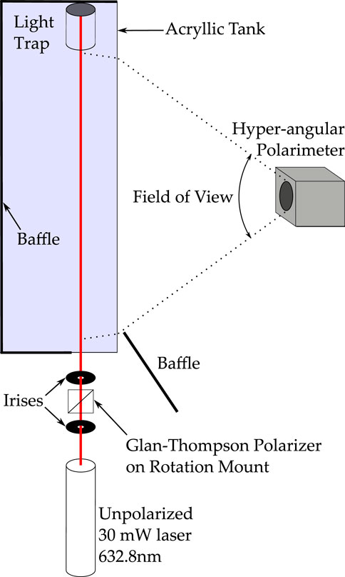
FIGURE 1. Schematic of the experimental setup.

In order to calibrate the rotation mount for the input polarizer, a second Glan-Thompson polarizer was placed such that its transmission axis was exactly perpendicular (90°) with respect to the surface of the optic table.

The laser was attenuated, directed through both polarizers, and the radiance measured with a spectrometer (QE-Pro, Ocean Optics). The mount angle was varied manually until the signal level was minimized, which determined the angular offset at which the transmission angle was exactly parallel with the optic table (0°). Positive polarizer angles are specified to be counter-clockwise with respect to this position, when looking into the beam.

The orientation of the laser with respect to the tank was adjusted in order to keep the influence of internal reflections within the tank as even as possible along the beam length. The zenith angle was aligned with the tank by first removing the light trap, and allowing the beam to transmit fully through the rear of the tank. The angle was adjusted until the beam height entering and exiting the tank were identical. Aligning the azimuth angle exactly parallel with the tank was not possible; it would have back-reflected the beam into the laser’s aperture, potentially damaging it. A small azimuthal misalignment was introduced to avoid this.

Mantis was placed on a table adjacent to the tank, and its front window was positioned 1.3 m away from the face of the tank. It was oriented on its side, such that the 72° FOV was horizontal. The instrument was attached to a vertical translation stage mounted to a tilting stage, thus allowing two degrees of freedom to align its FOV with the laser’s path. To perform the alignment, we replaced the beam trap with a diffusely reflecting white object, so that the beam created a bright spot of light near the rear of the tank. We then removed the exterior baffle indicated in Figure 1. As the beam transmits through the front wall of the tank, the scattering that occurs at the interface causes an additional bright spot at the location where the beam enterers the tank. In order to align the sensor FOV with the beam, the vertical position and tilt of Mantis were adjusted until the signal level from both bright spots (the front and rear of the beam) were simultaneously maximized, ensuring that every pixel along the beam’s length was viewing the brightest, central part of beam profile.

For this experiment, our goal was to retrieve the Mueller matrix of two specific polystyrene particle standards, with diameters of 0.994 and 4.0 μm (3K-990, 4K-04, ThermoFisher Scientific). Since we planned to isolate the scattering signal due to the particles, we chose to use tap water as the scattering medium. The use of pure water was considered, but due to the volume of water required (≈535 L) and the surface area of the tank, maintaining the purity of the water was deemed too difficult. We also were interested to contrast the Mueller matrix of the tap water signal with the theoretical Mueller matrix for pure water.

After thoroughly cleaning the interior, the tank was filled to a 90% level with tap water and allowed to settle and degas for 48 h. After this period, a dusting of large particles was visible on the floor of the tank, the water had warmed to room temperature ($\approx 19°C$), and no bubbles were visible on the walls of the tank. To remove the large particulates, the tank water was recirculated through two inline water filters, a 5.0 μm, followed by a 1.0 μm for 4 h, and then allowed to settle for a further 24 h. The ac-9 instrument was gently submerged in the tank, and a set of absorption (a) and attenuation (c) coefficients were collected and linearly interpolated to 632.8 nm. After appropriate instrumental corrections (Stockley et al., 2017), the scattering coefficient (b) is calculated as b = c − a.

To perform the tap water background measurement, all internal lights in the room were turned off. Both the laser and Mantis were switched on and allowed to stabilize for 15 min, and the input polarizer was rotated to the horizontal position (0°). Due to the small magnitude of scattered light, the collection parameters were adjusted to maximize the collected signal: the sensor integration time was set to 1 s, and the number of polarizer rotations averaged for one measurement was set to 8. Since the sensor collects 16 frames per rotation during a measurement, this means that each acquisition integrated for approximately 128 s (Foster et al., 2020). First, the sensor aperture was covered and several dark offset frames were collected. Once complete, the aperture was uncovered and a series of 8 measurements were made, rotating the input polarizer by 22.5° in between each one. The choice of 8 angles is explained in Section 2.4 and is visualized in Figure 3.

Proceeding the background measurement, one bottle (5 ml) of the 4.0 μm bead solution was gently mixed into the 535 L of sample volume until uniformly distributed. The ac-9 instrument was again used to measure the total absorption and scattering coefficient of the solution. As a cross check on the optical properties, the total number of particles (N_p) in the sample volume was calculated using the manufacturer-provided formula (Thermo Fisher Scientific, 2018), and Mie calculations (described in section 3) provided a scattering cross section (C_sca). The measured (0.015 m⁻¹) and theoretical bead scattering coefficient, calculated as b = N_pC_sca/0.535 m³, agreed to within 20% which is typical for these type of measurements (Stockley et al., 2017). After collection of another set of dark spectra, the series of 8 collections were performed again, using the same generator angles as for the background water measurement. Once all desired measurements were complete, the tank was drained and thoroughly cleaned.

The second experiment was repeated in exactly the same manner. This time, one bottle (5 ml) of the 0.994 μm bead solution was mixed into the sample volume, for a theoretical bead scattering coefficient of 0.86 m⁻¹. As will be seen in section 3, the significantly higher scattering coefficient, and therefore signal-to-noise ratio (SNR), may explain some of the differences in inversion results for the smaller vs. larger bead solution.

At a later date, LISST-VSF measurements of tap water and 0.994 μm beads were collected for comparison with inversion results. In order to replicate the original experiment conditions as closely as possible, flushed tap water from the same faucet was allowed to degas in a 2 L glass beaker for 24 h. The water was poured into the black sample chamber of the instrument and allowed to settle for 3 h. Two sets of 100 measurement were collected. Following the tap water measurements, 12.4 μL of 0.994 μm bead solution was mixed into the sample chamber in order to approximate the particle concentration of the original experiment, and two more sets of 100 measurements were collected. In order to increase the SNR of the measurement, an additional 12.4 μL of bead solution was added to the sample chamber (for a total of 24.8 μL) and the collections repeated. Following quality control of the measurements, median data at each scattering angle were determined and appropriate corrections were applied based on recommendations from Koestner et al. (2018), Koestner et al. (2020). In brief, the corrections refer to angle-dependent adjustments to the outputs from manufacturer provided data processing code and are based on laboratory measurements and Mie scattering calculations for monodisperse polystyrene bead suspensions. These corrections were found to be necessary in previous studies and have been validated with independent measurements (Koestner et al., 2018).

2.3 Radiative Transfer Calculations

For this section, it is helpful to refer to the scattering diagram given in Figure 2 and the list of symbol definitions in Table 1. In order to simply the math that follows, ΔV is considered to be a rectangular cuboid, which closely approximates the projection of the pixel FOV upon the volume illuminated by the laser beam, and dV is a differential element of that same volume. When viewing the beam at 90°, each pixel sees a distance along the beam of 1 mm. Since the pixel FOV is smaller than the beam cross section, each pixel sees a cuboid of roughly (1 mm × 3 mm x 1 mm), where 3 mm is the full width of the beam profile (in the $\widehat{y}$ direction as depicted in Figure 2). This volume increases as the viewing angle becomes more oblique.

FIGURE 2

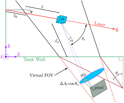
FIGURE 2. Illustration of the scattering geometry for a single pixel FOV. Figure symbols enlarged.

TABLE 1

TABLE 1. List of symbols used in this work.

In its most basic form, the differential equation governing the scattering of light from the elementary volume dV is given by

$dJ=\left[b\tilde{\beta }\left({\theta }_s\right)\right]EdVd{\mathrm{\Omega }}^{\prime }dtd\lambda ,\left[J\right](1)$

where θ_s is the scattering angle, dΩ′ (sr⁻¹) is the elementary solid angle receiving the scattered light, E (W m⁻² nm⁻¹) is the spectral irradiance incident upon dV, b (m⁻¹) is the scattering coefficient, $\tilde{\beta }({\theta }_s)({\mathrm{s}\mathrm{r}}^{-1})$ is the scattering phase function, t (s) is time, and λ (nm) is wavelength. In short, dJ is the energy in Joules leaving dV at angle θ_s and flowing into solid angle dΩ′, per unit time and wavelength.

However, dJ/dt = dΦ, the radiant flux, and further, dΦ/dλ is the optical power. We can thus re-arrange Eq. 1 as

$\frac{d\mathrm{\Phi }}{d\lambda }=\left[b\tilde{\beta }\left({\theta }_s\right)\right]EdVd{\mathrm{\Omega }}^{\prime }\left[\frac{\mathrm{W}}{\mathrm{n}\mathrm{m}}\right].(2)$

Let us now include the Stokes vector formalism for light polarization. For mathematical reasons, we will consider Φ and E as abstract constructs representing coherent Stokes vectors of the radiant flux and spectral irradiance, respectively. The notion of a Stokes vector for flux or irradiance does not make physical sense without considering a direction of energy flow, but this will come later. The scattering phase function now becomes the (4 × 4) scattering phase matrix, $\tilde{\mathit{\beta }}({\theta }_s)({\mathrm{s}\mathrm{r}}^{-1})$, and when multiplied by the scattering coefficient it becomes the volume scattering matrix, β(θ_s) (m⁻¹sr⁻¹). For generality, we must also include two Stokes vector rotation matrices, R₁ and R₂, which rotate the Stokes vector reference plane into and out of the scattering plane:

$\mathit{R}\left(\theta \right)=\left[\begin{array}{cccc}\hfill 1\hfill & \hfill 0\hfill & \hfill 0\hfill & \hfill 0\hfill \\ \hfill 0\hfill & \hfill \cos 2\theta \hfill & \hfill -\sin 2\theta \hfill & \hfill 0\hfill \\ \hfill 0\hfill & \hfill \sin 2\theta \hfill & \hfill \cos 2\theta \hfill & \hfill 0\hfill \\ \hfill 0\hfill & \hfill 0\hfill & \hfill 0\hfill & \hfill 1\hfill \end{array}\right].(3)$

For the geometry of the presented experiment, the scattering plane and the Stokes vector meridional plane are orthogonal to each other, leading to θ = 90° for both R₁ and R₂.

We now have

$\frac{d\mathbf{\Phi }}{d\lambda }={\mathit{R}}_2\left[b\tilde{\mathit{\beta }}\left({\theta }_s\right)\right]{\mathit{R}}_1\mathit{E}dVd{\mathrm{\Omega }}^{\prime }\left[\frac{\mathrm{W}}{\mathrm{n}\mathrm{m}}\right].(4)$

Consider now the spectral irradiance (E) which is incident upon dV. E depends on the laser output power (Φ), the beam cross section (A_b), the total optical depth between the laser aperture and dV, the cross-sectional area which dV subtends within the beam (A_c), as well as transmission through the tank walls (mostly influencing the polarization). The flux passing through A_c will decrease with distance from the front of the tank (ℓ₀), not only because of attenuation over the optical path length, but also because the beam diverges with distance and therefore A_c occupies a decreasing fraction of the total beam area. Estimating this fraction is difficult, but is done geometrically, accounting for refraction of the FOV through the tank walls, and for the diverging Gaussian beam profile. In the end, we calculate that A_c intercepts 65% of the radiant flux in the beam profile near the front of the tank, decreasing to 30% at the largest path lengths. Further details about this calculation may be found in the Supplementary Material for this article.

Denoting this fraction as f(ℓ₀), T₁ and T₂ as the Fresnel transmission matrices from air to acrylic glass, and from acrylic glass to water, the spectral irradiance impinging on dV can be expressed as

$\mathit{E}=f\left({\ell }_0\right)e^{-c\left({\ell }_0+\ell \right)}{\mathit{T}}_2{\mathit{T}}_1\frac{\mathbf{\Phi }}{A_b\mathrm{\Delta }\lambda }\left[\frac{\mathrm{W}}{{\mathrm{m}}^2\mathrm{n}\mathrm{m}}\right],(5)$

where the optical depth is given by the attenuation coefficient c multiplied by ℓ₀. Explicit dependence on the wavelength and incidence angle have been omitted for clarity, and we have further assumed that the Stokes vector of the incident light is unchanged when propagating through the intervening air, tank walls and the water. It is likely that the incident light becomes increasingly depolarized as it traverses the tank, which can contribute to some discrepancies at the largest path lengths. Multiple reflections between or within the tank walls have not been considered.

The initial flux Φ₀ is formed by passing an unpolarized laser with output flux Φ through a Glan-Thompson polarizer mounted to a rotation stage. The Mueller matrix for a linear polarizer oriented at 0° with polarized intensity transmittances parallel to (t_ℓ) and perpendicular to (t_r) the polarizer axis is given by Chipman (1995):

$\mathit{P}\left(0°,{\mathit{t}}_{\mathit{\ell }},t_r\right)=\frac{1}{2}\left[\begin{array}{cccc}\hfill t_{\ell }+t_r\hfill & \hfill t_{\ell }-t_r\hfill & \hfill 0\hfill & \hfill 0\hfill \\ \hfill t_{\ell }-t_r\hfill & \hfill t_{\ell }+t_r\hfill & \hfill 0\hfill & \hfill 0\hfill \\ \hfill 0\hfill & \hfill 0\hfill & \hfill 2\sqrt{t_{\ell }{t}_r}\hfill & \hfill 0\hfill \\ \hfill 0\hfill & \hfill 0\hfill & \hfill 0\hfill & \hfill 2\sqrt{t_{\ell }{t}_r}\hfill \end{array}\right],(6)$

which can be generalized to a polarizer oriented with arbitrary axis angle η through

$\mathit{P}\left(\eta ,t_{\ell },t_r\right)=\mathit{R}\left(\eta \right)\mathit{P}\left(0°,{\mathit{t}}_{\ell },t_r\right)\mathit{R}\left(-\eta \right).(7)$

Thus, the polarization angle of the incident flux is modulated by the position of the polarizer, such that

${\mathbf{\Phi }}_0=\mathit{P}\left(\eta \right){\mathit{S}}_0=\mathit{P}\left(\eta \right){\left[\begin{array}{cccc}\hfill \mathrm{\Phi }\hfill & \hfill 0\hfill & \hfill 0\hfill & \hfill 0\hfill \end{array}\right]}^T\left[W\right],(8)$

where we again drop explicit dependence on the polarizer properties and rotation angle from Φ₀ to simplify the notation.

The light scattered from dV must travel a distance ℓ_s before it reaches the edge of the tank, experiencing an attenuation of $e^{-c{\ell }_s}$, as well as an apparent attenuation   cos(α), where α is the angle between the center of the field of view and dΩ′. Upon reaching the tank wall, it must refract twice [water to acrylic glass (T₃), and then finally acrylic glass to air (T₄)]. Combining Eqs 4, 5, the full differential equation governing the experiment is:

$\frac{d\mathbf{\Phi }}{d\lambda }=f\left({\ell }_0\right)\frac{e^{-c\left({\ell }_0+\ell +{\ell }_s\right)}}{A_b}\cos \left(\alpha \right){\mathit{T}}_4{\mathit{T}}_3{\mathit{R}}_2\left[b\tilde{\mathit{\beta }}\left({\theta }_s\right)\right]{\mathit{R}}_1{\mathit{T}}_2{\mathit{T}}_1{\mathbf{\Phi }}_{0}dVd{\mathrm{\Omega }}^{\prime }\left[\frac{\mathrm{W}}{\mathrm{n}\mathrm{m}}\right].(9)$

To determine the radiant flux received by the pixel, we need to consider the contributions from all parts of the beam in view of the pixel. This is an integration over the beam volume within the FOV (ΔV) and over the solid angle subtended by the pixel’s entrance pupil (ΔΩ′):

$\frac{\mathbf{\Phi }}{\mathrm{\Delta }\lambda }={\int }_{\mathrm{\Delta }V}{\int }_{\mathrm{\Delta }{\mathrm{\Omega }}^{\prime }}f\left({\ell }_0\right)\frac{e^{-c\left({\ell }_0+\ell +{\ell }_s\right)}}{A_b}\cos \left(\alpha \right){\mathit{T}}_4{\mathit{T}}_3{\mathit{R}}_2\left[b\tilde{\mathit{\beta }}\left({\theta }_s\right)\right]{\mathit{R}}_1{\mathit{T}}_2{\mathit{T}}_1{\mathbf{\Phi }}_{0}d{\mathrm{\Omega }}^{\prime }dV\left[\frac{\mathrm{W}}{\mathrm{n}\mathrm{m}}\right].(10)$

Almost all of the parameters in Eq. 10 are functions of ℓ, including the scattering angle, which makes the integration quite difficult. If we make the reasonable assumption of homogeneity across a pixel (which, as mentioned above samples ≈ 1 mm of beam length) then ℓ, ℓ_s, f(ℓ₀), and θ_s can be treated as constants within a pixel, and   cos(α) ≈ 1. Further, in the paraxial approximation, we can substitute dΩ′ = dA_l  cos θ_v/D², where dA_l  cos θ_v is the differential entrance pupil area receiving the flux, and D is the distance (accounting for refraction) from dV to the lens.

The solution can then be approximated as

$\frac{\mathbf{\Phi }}{\mathrm{\Delta }\lambda }\approx f\left({\ell }_0\right)e^{-c\left({\ell }_0+\ell +{\ell }_s\right)}\frac{b\mathrm{\Delta }V\mathrm{\Delta }{A}_l}{D^2{A}_b}\cos \left({\theta }_v\right){\mathit{T}}_4{\mathit{T}}_3{\mathit{R}}_2\tilde{\mathit{\beta }}\left({\theta }_s\right){\mathit{R}}_1{\mathit{T}}_2{\mathit{T}}_1{\mathbf{\Phi }}_0\left[\frac{\mathrm{W}}{\mathrm{n}\mathrm{m}}\right].(11)$

And finally, the expected radiance (diffuse Stokes vector, S) is the spectral radiant flux divided by ΔA_l and the solid angle of the pixel’s field of view (ΔΩ_FOV):

$\mathit{S}\approx \frac{\mathbf{\Phi }}{\mathrm{\Delta }{A}_l\mathrm{\Delta }\lambda \mathrm{\Delta }{\mathrm{\Omega }}_{\text{FOV}}}\left[\frac{\mathrm{W}}{{\mathrm{m}}^2\mathrm{n}\mathrm{m}\mathrm{s}\mathrm{r}}\right].(12)$

2.4 Inversion of the Mueller Matrix

Since detectors are only sensitive to light intensity, polarimetric data reduction techniques are formulated so that they operate on intensity measurements of light fully polarized in a specific direction (e.g., I₀, I₄₅, I₉₀, … etc.). This makes sense for experiments where a calibrated detector provides measurements directly proportional to the polarized intensities. In fact, often the raw digital number (DN) may be substituted directly, if the quantity of interest does not depend on the absolute magnitude of the signal, which is the case for all Mueller matrix elements except for the phase function. In this experiment we do not have that option. Mantis acquires Stokes vectors by modulating the intensity measurements through a constantly rotating polarizer (polarization modulation approach), and thus the raw intensity measurements are not directly proportional to the polarized intensities (Foster et al., 2020). The Stokes vector is inverted directly from the modulation, and thus represents the lowest level data product.

To estimate the parameters of the scattering Mueller matrix ($\tilde{\mathit{\beta }}$) using Mantis, we tailor the polarimetric data reduction technique for operation directly on Stokes vectors. As originally conceived by Azzam (1978) and using the nomenclature of Chipman (1995), a Mueller matrix can be inverted from a set of N intensity measurements if the system is linear and the n-th intensity is of the form ${\mathit{P}}_n=k{\vec{\mathit{A}}}_n\tilde{\mathit{\beta }}{\mathit{S}}_n$, where k is a scaling constant, ${\vec{\mathit{A}}}_n$ is the n-th analyzer vector (first row of the system Mueller matrix for all optical components in-between the sample and the photodetector), and S_n is the n-th incident Stokes vector. Since Mantis is only able to measure the linear Stokes components (S = [I Q U]^T), we limit our discussion to the (3 × 3) Mueller matrix.

To be able to use the technique, we reform $\tilde{\mathit{\beta }}$ into a (9 × 1) Mueller vector ($\vec{\mathit{\beta }}$):

$\vec{\mathit{\beta }}={\left[\begin{array}{ccccccccc}\hfill {\tilde{\beta }}_{11}\hfill & \hfill {\tilde{\beta }}_{12}\hfill & \hfill {\tilde{\beta }}_{13}\hfill & \hfill {\tilde{\beta }}_{21}\hfill & \hfill {\tilde{\beta }}_{22}\hfill & \hfill {\tilde{\beta }}_{23}\hfill & \hfill {\tilde{\beta }}_{31}\hfill & \hfill {\tilde{\beta }}_{32}\hfill & \hfill {\tilde{\beta }}_{33}\hfill \end{array}\right]}^T\left[{\mathrm{s}\mathrm{r}}^{-1}\right].(13)$

Using the Mueller vector, a scattered Stokes vector, S_sca, is expressed in terms of the incident Stokes vector as

${\mathit{S}}_{\text{sca}}=\left[\begin{array}{ccccccccc}\hfill I\hfill & \hfill Q\hfill & \hfill U\hfill & \hfill 0\hfill & \hfill 0\hfill & \hfill 0\hfill & \hfill 0\hfill & \hfill 0\hfill & \hfill 0\hfill \\ \hfill 0\hfill & \hfill 0\hfill & \hfill 0\hfill & \hfill I\hfill & \hfill Q\hfill & \hfill U\hfill & \hfill 0\hfill & \hfill 0\hfill & \hfill 0\hfill \\ \hfill 0\hfill & \hfill 0\hfill & \hfill 0\hfill & \hfill 0\hfill & \hfill 0\hfill & \hfill 0\hfill & \hfill I\hfill & \hfill Q\hfill & \hfill U\hfill \end{array}\right]\vec{\mathit{\beta }}=\left(\mathcal{I}\otimes {\mathit{S}}_{\text{inc}}^T\right)\vec{\mathit{\beta }},(14)$

where ⊗ denotes the Kronecker tensor product, and $\mathcal{I}$ is the (3 × 3) identity matrix.

The resiliency of the inversion depends on how well-conditioned the problem is, and this is the reason why considerable attention is given to the careful selection of the N sampling points on the Poincaré sphere (Goudail and Dai, 2020). If exactly N = 9 sufficiently separated points are chosen (or 16 in the case of the (4 × 4) Mueller matrix), the system can be represented as

$\mathcal{P}=k\mathit{W}\vec{\mathit{\beta }}=k\left[\begin{array}{c}\hfill {\vec{\mathit{A}}}_1\otimes {\mathit{S}}_1^T\hfill \\ \hfill {\vec{\mathit{A}}}_2\otimes {\mathit{S}}_2^T\hfill \\ \hfill {\vec{\mathit{A}}}_3\otimes {\mathit{S}}_3^T\hfill \\ \hfill ⋮\hfill \\ \hfill {\vec{\mathit{A}}}_N\otimes {\mathit{S}}_N^T\hfill \end{array}\right]\vec{\mathit{\beta }},(15)$

with $\vec{\mathit{\beta }}$ being uniquely determined using a standard matrix inversion, i.e. $\vec{\mathit{\beta }}={\mathit{W}}^{-1}\mathcal{P}$. If the system is over-determined (N $>$ 9), a Moore-Penrose pseudo-inverse can be used, providing the minimum-norm, least-squares estimate of the Mueller matrix:

$\vec{\mathit{\beta }}=k{\mathit{W}}^{+}\mathcal{P}=k{\left({\mathit{W}}^T\mathit{W}\right)}^{-1}{\mathit{W}}^T\mathcal{P}.(16)$

However, in all such cases the vector $\mathcal{P}$ is a set of intensity measurements (Stokes I components only), which is incompatible with the measurement modality of the Mantis instrument. Instead, we operate on the full Stokes vector simultaneously, treating each Stokes component as an independent “intensity” measurement (row) in $\mathcal{P}$. Thus, we can no-longer treat $\vec{\mathit{A}}$ as a vector, but require the (3 × 3) Mueller matrix.

Let us denote S_n as the polarized radiance incident upon dV when the polarization state generator is rotated to the n-th position. The corresponding background-corrected Stokes vector measurement acquired by the Mantis instrument is denoted ${\mathcal{S}}_n^{\text{m}}$. We can combine Eqs 8, 11, 12 into the following form:

${\mathcal{S}}_n^{\text{m}}=k{\mathit{A}}_n\tilde{\mathit{\beta }}{\mathit{S}}_{n,}\left[\mathrm{W}{\mathrm{m}}^{-2}{\mathrm{n}\mathrm{m}}^{-1}{\mathrm{s}\mathrm{r}}^{-1}\right](\mathrm{17a})$

$k=f\left({\ell }_0\right)e^{-c\left({\ell }_0+\ell +{\ell }_s\right)}\frac{b\mathrm{\Delta }V}{D^2{A}_b\mathrm{\Delta }{\mathrm{\Omega }}_{\text{FOV}}},\left[{\mathrm{m}}^{-2}{\mathrm{s}\mathrm{r}}^{-1}\right](\mathrm{17b})$

${\mathit{A}}_n={\mathit{T}}_4{\mathit{T}}_3{\mathit{R}}_2(\mathrm{17c})$

${\mathit{S}}_n={\mathit{R}}_1{\mathit{T}}_2{\mathit{T}}_1\mathit{P}\left(\eta \right){\left[\begin{array}{ccc}\hfill {\mathrm{\Phi }}_0\hfill & \hfill 0\hfill & \hfill 0\hfill \end{array}\right]}^T\left[\mathrm{W}{\mathrm{n}\mathrm{m}}^{-1}\right](\mathrm{17d})$

In terms of the Mueller vector, we can write

${\mathcal{S}}_n^{\text{m}}=\left[\begin{array}{c}\hfill I_n^m\hfill \\ \hfill Q_n^m\hfill \\ \hfill U_n^m\hfill \end{array}\right]=k\left({\mathit{A}}_n\otimes {\mathit{S}}_n^T\right)\vec{\mathit{\beta }}=k{\mathit{W}}_n\vec{\mathit{\beta }}.(18)$

For N generator positions, we acquire a measurement vector $\mathcal{P}$ of size 3N, which is an improvement in efficiency compared to methods which are only able to leverage intensity measurements. With N = 3, a unique solution is found using a standard matrix inverse, but this is not preferable from a numerical standpoint, since the matrix condition number for such an inversion can be high depending on the specific generator angles chosen. Also, there are correlations among the I, Q, and U components for each generator position which arise because of external influences such as transmission through the tank walls, and non-ideality of the generator. It is therefore preferable to over-determine the system.

We have chosen N = 8 sampling points as a reasonable compromise between inversion accuracy and time required to complete an acquisition. Figure 3 illustrates the 8 points on the Poincaré circle for linear polarization (the equator of the Poincaré sphere). Having passed through the generator, the incident beam is fully polarized, and thus all of the points exist on the edge of the Poincaré circle (DoLP = 1). The angle of polarization (AoP) is shown graphically next to each point for context. The matrix condition number for the inversion is related to the size of the blue area within the circle. Borrowing the terminology of Tyo et al. (2010), a large blue region indicates that the measurement vectors which project the high dimensional “scene” space (the physics) into a low dimensional “sensor” space are highly orthogonal, and thus an accurate estimation of the physics can be reconstructed from the measurements without much loss of precision. The orange area is therefore proportional to the loss in precision. If the incident radiation were to become partially depolarized before impinging on the scattering volume, the loss of precision would be roughly proportional to the square of the degree of linear polarization (DoLP), since the radius of each point corresponds to the DoLP and the blue area would shrink by a factor of roughly DoLP².

FIGURE 3

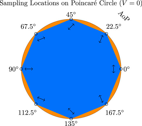
FIGURE 3. The location of the 8 sampling points (generator positions) on the Poincaré circle of linear polarization (V = 0). The orientation angle is given on the azimuthal axis, as well as shown graphically next to each point. The blue area is proportional to the precision with which the inversion is possible.

With N = 8 sampling points, W becomes a (24 × 9) matrix, which is inverted with a Moore-Penrose pseudo-inverse to obtain the Mueller vector:

$\mathcal{P}=\left[\begin{array}{c}\hfill {\mathcal{S}}_1^{\text{m}}\hfill \\ \hfill {\mathcal{S}}_2^{\text{m}}\hfill \\ \hfill ⋮\hfill \\ \hfill {\mathcal{S}}_8^{\text{m}}\hfill \end{array}\right]=k\mathit{W}\vec{\mathit{\beta }}=k\left[\begin{array}{c}\hfill {\mathit{A}}_1\otimes {\mathit{S}}_1^T\hfill \\ \hfill {\mathit{A}}_2\otimes {\mathit{S}}_2^T\hfill \\ \hfill ⋮\hfill \\ \hfill {\mathit{A}}_8\otimes {\mathit{S}}_8^T\hfill \end{array}\right]\vec{\mathit{\beta }},(19)$

$\vec{\mathit{\beta }}=k{\mathit{W}}^{+}\mathcal{P}=k{\left({\mathit{W}}^T\mathit{W}\right)}^{-1}{\mathit{W}}^T\mathcal{P}.(20)$

2.5 Symmetry Relationships

The technique described in Section 2.4 may be used to determine all 9 of the Mueller matrix elements under consideration. In the implementation thus far, each row of Mueller matrix elements is treated as linearly independent of the others. This approach works mathematically, but is not optimal. We can improve the quality of the inversion by utilizing knowledge about the structure of the scattering matrix. Primarily, we have a-priori knowledge about the symmetry relationships between the Mueller matrix elements.

The classic work of van de Hulst (1957) has shown that when a cloud of one kind of scatterers contains an equal amount of particles and their mirror particles and are randomly oriented, the resulting Mueller matrix contains 6 (out of 16) non-zero terms. Since we are not measuring (or generating) the V component, only 4 of them are invertible. Scattering by water molecules and by spherical microbeads satisfy these constraints (Hansen and Travis, 1974). Thus, when expressed in terms of the scattering angle we expect a matrix of the form

$\tilde{\mathit{\beta }}=\left[\begin{array}{ccc}\hfill {\tilde{\beta }}_{11}\hfill & \hfill {\tilde{\beta }}_{12}\hfill & \hfill 0\hfill \\ \hfill {\tilde{\beta }}_{12}\hfill & \hfill {\tilde{\beta }}_{22}\hfill & \hfill 0\hfill \\ \hfill 0\hfill & \hfill 0\hfill & \hfill {\tilde{\beta }}_{33}\hfill \end{array}\right]\left[{\mathrm{s}\mathrm{r}}^{-1}\right].(21)$

Immediately we can recognize the first symmetry relationship, ${\tilde{\beta }}_{12}={\tilde{\beta }}_{21}$.

In the case of molecular (Rayleigh) scattering, it is important to consider the anisotropy of the water molecules (Jonasz and Fournier, 2007), which causes a difference in polarized scattering behavior at scattering angles near 90° (Rayleigh, 1920). This is accounted for using a so-called depolarization factor, δ. For water molecules at θ_s = 90° scattering angle,

$\frac{{\tilde{\beta }}_{21}\left(90°\right)}{{\tilde{\beta }}_{11}\left(90°\right)}=\frac{1-\delta }{1+\delta }(22)$

The depolarization factor for pure water is estimated to be 0.039 (Farinato and Rowell, 1976). Thus, we can expect ${\tilde{\beta }}_{21}(90°)/{\tilde{\beta }}_{11}(90°)$ for scattering by molecular water to be on the order of 0.925. When the polystyrene beads are added to the sample volume, Mie theory predicts that ${\tilde{\beta }}_{22}={\tilde{\beta }}_{11}$, adding an additional symmetry we can leverage. This relationship is not used when depolarization is expected, to avoid introducing a bias into the result.

Another trivial, but useful observation is that four of the nine elements are zero. We can therefore introduce 4 more symmetry relationships: ${\tilde{\beta }}_{31}={\tilde{\beta }}_{13}$, ${\tilde{\beta }}_{32}={\tilde{\beta }}_{23}$, ${\tilde{\beta }}_{31}={\tilde{\beta }}_{32}$, and ${\tilde{\beta }}_{13}={\tilde{\beta }}_{23}$. These zero-relationships are important for the quality of the inversion. Without them, each of the zero terms may contain a small bias resulting from minor inaccuracies between measurements. By using these relationships, the zero terms become tightly coupled together. This reduces the individual bias of each zero term, thereby increasing the robustness of the remaining elements (Tyo et al., 2010).

From Eq. 21, we can observe that the ${\tilde{\beta }}_{33}$ element remains independent of the others, and cannot benefit from a symmetry relationship.

There are additional symmetries and relationships among the Mueller matrix elements that can be exploited (Fry and Kattawar, 1981; Cloude, 1990; Gil, 2000), but many of them are inequalities and would require use of a constrained least-squares technique or a different set of measurement angles (Tyo et al., 2010), which is reserved for future work. It is useful to observe that A_n also has the form of Eq. 21 which allows the elimination or simplification of many terms.

In order to leverage the symmetries in the inversion, we create additional “measurement” rows in both the ${\mathcal{P}}_n$ and W_n matrices, similar in spirit to that done in Tyo et al. (2010). The inclusion of each symmetry relationship adds an additional two rows to each. Algebraically, the new rows are formed by eliminating the row of W_n which does not have an impact upon the symmetry, and then swapping the columns which do correspond to the symmetry. An example for 4 different symmetry relationships is given in Eqs 23, 24. The ${\tilde{\beta }}_{12}={\tilde{\beta }}_{21}$ rows (changes shown in blue) are formed by removing the 3rd row of W_n (since it does not contribute to ${\tilde{\beta }}_{12}$ or ${\tilde{\beta }}_{21}$) and swapping the 2nd and 4th columns (corresponding to their position in $\vec{\mathit{\beta }}$). The additional rows for ${\mathcal{P}}_n$ are the corresponding Stokes components (I and Q, in this case).

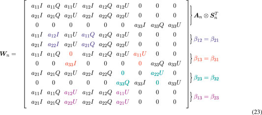
The corresponding set of measurements is given by

After accounting for the symmetries, each measurement point (one generator angle) results in a measurement matrix with 3 + 2Y rows, where Y is the number of symmetry relations used. After N = 8 sampling points, the total size of the W matrix to be inverted is [(24 + 16Y) × 9].

If only a subset of the Mueller matrix is required, the corresponding columns can simply be eliminated from W. Doing this can improve the quality of the inversion for the remaining elements, which is a possible design optimization (Tyo et al., 2010), but care must be taken to avoid introducing a bias into the result. We have observed a similar behavior with this inversion by omitting the columns corresponding to the zero Mueller matrix elements, essentially forcing them to be identically zero. However, given that the system is significantly over-determined already, the gain in fidelity was small, and we found the behavior of these elements to be a useful indicator of other problems with the setup or inversion technique. Depending on the particular elements desired, a smaller set of generator angles may be sufficient.

2.6 Angular Resolution

One further technique is used to increase the SNR of the inversion. The Mantis instrument has extremely high angular resolution (0.031° channel spacing), and our signals of interest do not contain spatial frequencies high enough to warrant the full use of this resolution. Theoretical calculations for the 0.994 and 4.0 μm microbeads indicate that the highest spatial period in the data under consideration is 7°, which occurs for the 4.0 μm beads (Figure 4). We chose to consider 15 spatial channels (pixels) together as one angular measurement, resulting in an effective channel spacing of $\approx 0.35°$, which still greatly exceeds the Nyquist frequency for this signal, leaving 20 sampling points (scattering angles) for each oscillation. Instead of inverting each high-resolution channel individually and simply binning every 15, we have chosen to combine the $\mathcal{P}$ and W matrices for each of the 15 channels, treating them as one combined inversion. This has several advantages over a naive binning approach, principally that the inversion is now a least-squares best fit to all 15 channels, and the symmetry relationships between all of the channels now work together to constrain the final result. In total, the size of the final W matrix becomes [(360 + 240Y) × 9]. When all the symmetry relationships are used (Y = 6), 1800 measurements contribute to inverting the 9 Mueller matrix elements for each scattering angle.

FIGURE 4

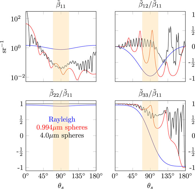
FIGURE 4. Theoretical phase matrices representing the three materials considered under this study. Rayleigh (blue), 0.994 μm microspheres (red), and 4.0 μm microspheres (black). The shaded region represents the range of scattering angles observable given the geometric constraints of the experimental setup.

3 Inversion Results and Discussion

In this section, we present the result of our Mueller matrix inversion for tap water and for two different polystyrene bead standards in comparison to theory, as well as a limited comparison with measurements made by the LISST-VSF instrument. Due to the geometric limitations of the experimental setup, only Mueller matrix elements for scattering angles between 74° and 115° are able to be inverted. Theoretical phase matrices for each of the three materials are given in Figure 4, where the retrievable scattering angles are denoted by the shaded region. Only the four unique Mueller matrix elements (Eq. 21) are shown in the figure.

3.1 Tap Water

As discussed above, it was unfeasible to fill the sample volume with 535 L of pure water and expect it remain pure enough to exhibit a Rayleigh-like phase function. Thus, for simplicity and ease of setup, tap water was used as the background medium. Since municipal tap water contains scatterers other than dipoles (minerals, sediment, etc.) and the exact composition is not known, it is of little value to compare it with a Rayleigh phase function. Some effort was made to fit the measured phase function to theoretical Mie calculations based on generic information provided by the local municipal water report. We varied the particle size and real refractive indices in combination with molecular scattering to get an approximate fit to the measured phase function, but this turned out to not work well enough for our needs. However, since the tap water visually exhibited signs of colloidal scattering (slightly cloudy appearance) and large particles were allowed to settle out, we hypothesized that the normalized Mueller matrix elements could exhibit a Rayleigh-like behavior consistent with Tyndall scattering (Jerlov and Kullenberg, 1953). Figure 5 illustrates the results, as compared with the normalized theoretical Rayleigh scattering matrix (Hansen and Travis, 1974) with the generally accepted depolarization ratio of 0.039 (Farinato and Rowell, 1976). All normalized elements match surprisingly well with Rayleigh scattering, despite the presence of other scatterers. The shape and relative magnitude between the measured and the Rayleigh scattering matrix agree across the full range of scattering angles. The high slope in the measured volume scattering function (VSF) is expected when there are non-dipole scatterers in the medium, and the leveling off of the magnitude near 105° is very likely caused by insufficient SNR for those longest path lengths. The mean value of β₂₂/β₁₁ was 0.945 4, which translates into a depolarization ratio of 0.028. The magnitude of the absolute percent differences between theory and measurement are on the order of 10%, except for β₁₃/β₁₁ and β₂₃/β₁₁ near 105° scattering angle. The exponential slope apparent in these elements are likely due to a mismatch in the scattering or absorption coefficients used in the inversion. The β₃₃/β₁₁ element matches the slope of the theoretical curve very well, up until the signal level begins to drop at 105°.

FIGURE 5

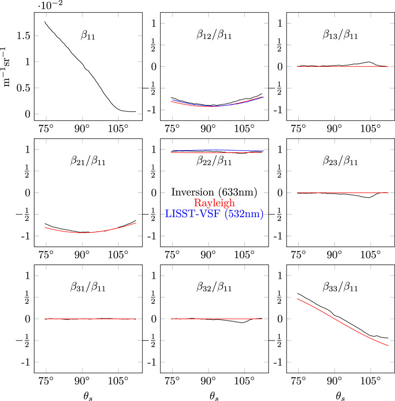
FIGURE 5. Scattering matrix inversion results for tap water, compared with the normalized Rayleigh scattering phase matrix using a depolarization ratio of 0.039. LISST-VSF measurements for tap water are shown for β₁₂/β₁₁ and β₂₂/β₁₁ The volume scattering function (β₁₁) is only shown for the inversion, since the water constituents were not characterized and there was a time difference between the two measurements.

Figure 5 also includes measurements of β₁₂/β₁₁ and β₂₂/β₁₁ made by the LISST-VSF instrument, at 532 nm. There was a significant time difference between the two measurements, which is why the phase functions are not comparable, however the Rayleigh-like behavior of the normalized elements is still maintained to a remarkable degree, even considering the wavelength difference. The excellent agreement between our inversion method with two different references (Rayleigh scattering theory and LISST-VSF measurement) is an important validation of our approach.

3.2 4.0 Micron Beads

When microbeads are added to the sample volume, we now have a reference for comparison of the scattering phase function (β₁₁). Since the scattering signal by the spheres is superimposed upon the background scattering signal from the water, the principle of incoherent superposition (Goldstein, 2003) allows us to isolate the sphere’s signal and compare it directly to theory. In order to determine the theoretical Mueller matrix for the microbeads, Mie calculations (de Rooij and van der Stap, 1984) were carried out using information from the specific sample bottle. The complex refractive index of the spheres was calculated using the manufacturer supplied formula for 475.3 nm (in-water equivalent of 632.8 nm), assuming negligible absorption. After adjusting relative to the refractive index of water, the result was 1.188 + j0. A two-parameter gamma particle size distribution (PSD) was used for the calculations, where the effective radius was 2.0 μm, and the effective variance was 0.000 4 μm². The average cosine of the phase function was 0.894. The scattering cross-section from the calculations is used along with the number of particles per mL to estimate the expected scattering coefficient in section 2.2.

For the first inversion attempt using beads, 5 ml of the 4.0 μm microbead solution was added to the sample volume. This solution was chosen because the theoretical curve exhibited a very distinctive, high spatial period oscillation within the angular range considered. However, as will be seen below, the larger beads present a much smaller scattering cross section and particle count, resulting in a much lower scattering coefficient and SNR complications. Additional bead solution was not available to increase the signal level.

The inversion result is shown in Figure 6. The phase function for the spheres turned out to have a reduced magnitude and diverging trend at the largest scattering angles when compared with the theoretical calculations. Despite this, there are several oscillations in the retrieved VSF which have a similar spatial period as the theoretical curve. Given that the signal level was lower than anticipated, this result is not entirely unexpected. Nevertheless, there is strong agreement between theory and measurement for all of the normalized Mueller matrix elements. β₁₂/β₁₁ and β₂₁/β₁₁ in particular, show excellent agreement in both angular frequency and magnitude across the angular range. The β₃₃/β₁₁ element has a slightly different slope as compared to theory. This mismatch suggests that the PSD parameters used for the theoretical curve may be different than the true distribution, however the general downward oscillatory trend of the data is maintained. Empirically, recalculating the theoretical curves with a slightly smaller mean diameter (e.g. 3.98 μm) brings the oscillations more in phase with the inversion, indicating that the true bead diameter may be smaller than anticipated. All other elements which are expected to be zero are in fact close to zero, with small artifacts which are likely due to the amplification of instrumental noise at the low signal levels involved.

FIGURE 6

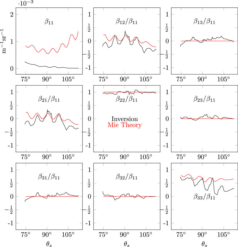
FIGURE 6. Inverted phase matrix compared with Mie scattering theory for 4.0 μm spheres.

3.3 0.994 Micron Beads

Based on lessons learned from the 4.0 μm beads, the final inversion used 5 ml of a 0.994 μm microbead solution in the sample volume. This solution provides a different set of challenges and opportunities compared to the 4.0 μm beads. The smaller beads produce a single, pronounced period with a wide dynamic range in the β₁₂/β₁₁ element. The same volume of bead solution also contains a significantly higher number of particles, which increases the scattering coefficient, and therefore the SNR of the measurements. For the theoretical calculations, the effective radius and variance were set to 0.497 μm and 0.000025 μm², respectively. The average cosine of the phase function was 0.920, a similar value to that of the 4.0 μm beads.

Figure 7 shows the inverted Mueller matrix elements for the 0.994 μm beads in comparison to theory. With more signal level, we can see that up through approximately 95°, the inversion is successful in replicating the theoretical VSF in both shape and magnitude, to within about 15%. The latter half of the VSF diverges in magnitude from the theory, but manages to preserve the angular frequency. Just as in the tap-water case, potential explanations include the amplification of small inaccuracies over the long path length, or simply a very minor misalignment of the sensor causing a flux different than predicted. The agreement between all of the normalized elements and the theory is excellent. In particular, the β₁₂/β₁₁ and β₂₁/β₁₁ elements agree with Mie theory almost perfectly at 90°, and slowly diverges to about a 20% difference at 75° and 115°. The β₂₂/β₁₁ element is flat across all scattering angles measured, with a mean of 0.951 5, compared to a theoretical value of 1.0 for homogeneous spheres. This value is only slightly higher than that observed in the tap water (0.945 4). Element β₃₃/β₁₁ clearly reproduces the angular features of the theory, with a slight over and undershoot at the maximum and minimum points. The measured curve exceeds 1 for some scattering angles, an unphysical result which is likely caused by the fact that β₃₃ cannot leverage any symmetry constraints; its only contributor is the U Stokes component, and thus is especially sensitive to it. All remaining elements are consistently zero for all measured scattering angles, to within 5%.

FIGURE 7

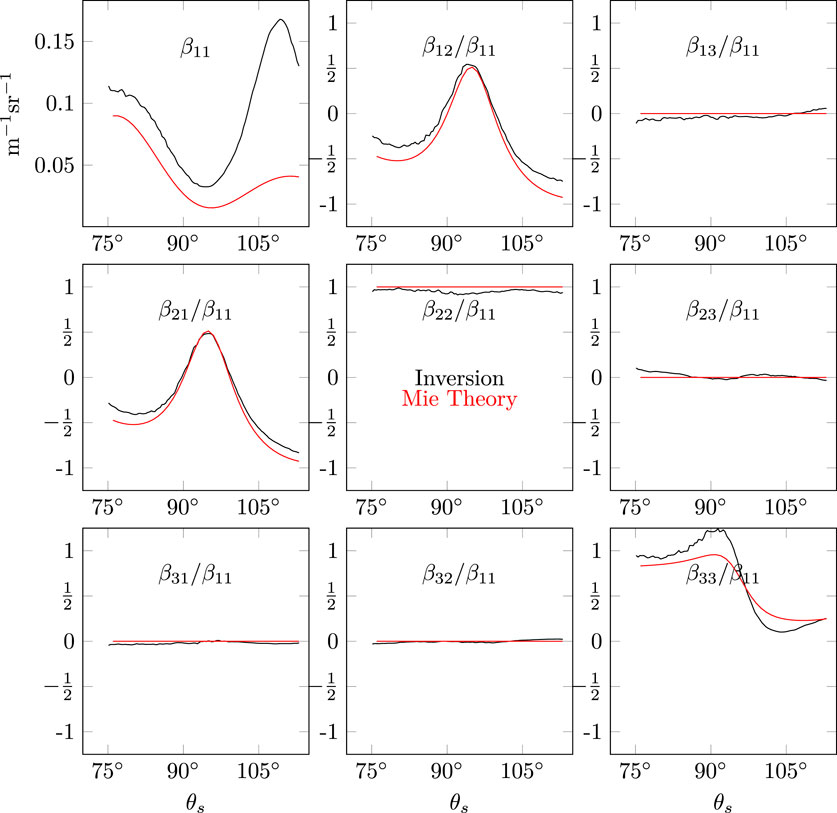
FIGURE 7. Inversion result compared with Mie theory for 0.994 μm beads.

Similar to the tap-water results above, measurements made by a LISST-VSF at a later date are shown in Figure 8. The Mie results are calculated at 398nm, corresponding to the 532 nm in-air wavelength of the LISST-VSF. This conversion was not needed for the tap-water case because the Rayleigh phase matrix is not wavelength dependent. To eliminate uncertainties associated with differences in bead concentrations, the LISST-VSF phase function was multiplied by the bead scattering coefficient from the original experiment to form the VSF in the figure. The impact of the different wavelengths can be clearly observed in the shape of the VSF, and of the β₁₂/β₁₁ element. Both instruments replicate the shape and magnitude of the VSF predicted by the theory, including the distinctive shift in peak location with wavelength. The β₁₂/β₁₁ element also agrees quite well, with the LISST-VSF successfully reproducing both the spatial period and peak locations of theory, but slightly underestimating the peak magnitude—a fact already observed for a suspension of polystyrene beads (Koestner et al., 2018). Both techniques are able to reproduce the flat shape of β₂₂/β₁₁ across all angles, with the LISST-VSF producing a mean value of 0.987 5. The general agreement in magnitude and trend among all elements and with measurements from a commercially available instrument further validates the inversion methodology.

FIGURE 8

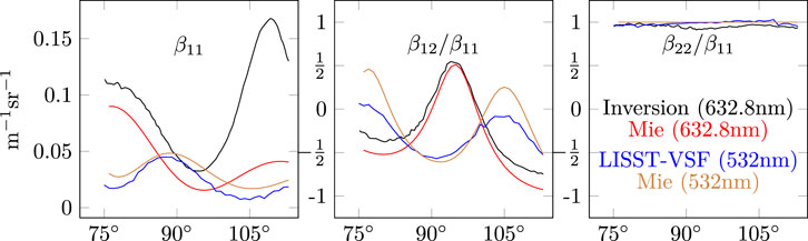
FIGURE 8. Inverted β₁₁, β₁₂/β₁₁ and β₂₂/β₁₁ elements and LISST-VSF measurement compared with Mie theory for 0.994 μm spheres.

4 Challenges and Opportunities

The technique presented in this work demonstrates a method of obtaining information about the polarimetric scattering properties of hydrosols without the use of dedicated, potentially expensive instrumentation designed for the task. Although our goal was to demonstrate a proof-of-concept, the success of the technique paves the way for future studies where greater control over the experimental parameters and sample properties are possible. Multiple variations are possible. For example, with an appropriate wide-angle lens and compact imaging polarimeter, we can envision a portable version of this setup with a much smaller sample volume for use in the field or on research vessels. Inclusion of the Fresnel effects into the inversion opens up the possibility of outdoor installations, where a polarimeter images the scattered light from across the air-sea interface. Of course, this introduces a plethora of additional challenges, not limited to accounting for the wind-driven ocean surface and contamination from other light sources. These difficulties could be partially mitigated by operating the system in calm conditions, either at night or with appropriate background-rejection techniques. Such a setup would be most useful for examining the normalized Mueller matrix elements, which are more robust to variations in the host medium, and the constant terms shown in Eq. 17a become less important, since they cancel out during the normalization. Other light sources could also be considered; we used a red laser because it was available, was unpolarized, and had sufficient output power. Green, blue, or even ultra-violet lasers could provide interesting insights into the spectral scattering behavior of hydrosols.

The SNR of the measurements plays a critical role in the success of the technique. The scattering coefficient of the 4.0 μm beads (b = 0.015 m⁻¹) was perhaps the lower limit, considering the noise present in the result. Lower concentrations are certainly possible, but would require either a more sensitive instrument than Mantis, or a more powerful laser. There was possibly too much signal for the 0.994 μm beads (b = 0.86 m⁻¹); considering that the total path length for the furthest scattering angles was 1.4 m, the total optical depth was nearly 1.7. According to Bohren (1987), the single-scattering regime can be expressed as (in our case) c(ℓ₀ + ℓ + ℓ_s)(1 − g) ≪ 1, where g is the average cosine of the phase function. The highest value of the expression is 0.15 for the 0.994 μm beads, and 0.07 for the 4.0 μm beads. Arguably, the 0.994 μm beads may have been impacted by multiple scattering to a small degree, possibly explaining the discrepancies observed for larger scattering angles in the phase function. The magnitude of the effect may also depend on the actual phase function of the scatterers (Jonasz and Fournier, 2007).

Although our experiment targets scattering angles near 90°, a different angular range is equally plausible by changing the orientation of the polarimeter with respect to the tank. This may be useful for comparison with commercial single-angle backscatter devices, or for determining the particulate backscattering coefficient (Sullivan and Twardowski, 2009). Measurements made in the near-forward scattering regime could examine how light is depolarized by seawater or the presence of specific hydrosols (Gorodnichev et al., 2020). For near-backscattering angles, this scheme could provide insight into the relationship between the LIDAR depolarization ratio [i.e., β₂₂(180°)/β₁₁(180°)] and particle size and composition (Burton et al., 2015). Some considerations for applying this technique to other measurement geometries include: 1) for near-forward scattering angles, the dynamic range of the polarimeter used may become a limiting factor, 2) for near-backward scattering angles, the signal level may be too low or require a long integration time, 3) for very long path lengths, multiple scattering may become a concern, or 4) for oblique viewing angles, the scattered signal may be totally internally reflected by the tank walls. The latter point is salient when considering hydrosol scattering in a natural environment, since only specific scattering angles are able to transmit through the air-sea interface (Ibrahim et al., 2012). A specially designed sample chamber that could accommodate several compact polarimeters at different viewing angles could potentially acquire a much larger range of scattering angles simultaneously.

5 Conclusion

In this work, we have successfully demonstrated that a passive polarimeter, in combination with a laser light source and linear polarizer, is able to accurately invert 9 of the 16 elements of the scattering Mueller matrix. We have derived the necessary radiative transfer equations to obtain an accurate forward model of the system, accounting for the impact of refraction of both the incident and scattered flux on the polarization state of the beam. The polarimetric data reduction technique of Azzam (1978) and Chipman (1995) was modified to accommodate the direct Stokes vector output of the polarimeter in lieu of intensity measurements, and allowed for the natural symmetry among elements of the scattering Mueller matrix. Measurements of tap water, 0.994 μm, and 4.0 μm microbead solutions were made using 8 different linear polarization angles. The inversion methodology was applied to all datasets and favorably compared with theoretically calculated Mueller matrices of Rayleigh scattering and Mie theory. Additional measurements with a commercial LISST-VSF instrument corroborate the results and validate the approach. The inversion framework presented in this paper enables the possibility of Mueller matrix polarimetry using passive remote sensing instrumentation, and hopefully will lead to an increased density of Mueller matrix measurements in the literature.

Data Availability Statement

The raw data supporting the conclusions of this article will be made available by the authors, without undue reservation.

Author Contributions

RF designed and performed the experiment, analyzed the data, designed the inversion methodology and calculations, and wrote the first draft of the manuscript. DG provided equipment and consultation. DK performed the LISST-VSF measurements and contributed sections of the manuscript. AE-H performed Mie scattering calculations. JB provided consultation and funding. RF, DK, and AE-H contributed to manuscript revision, read, and approved the submitted version.

Funding

Office of Naval Research (ONR); National Aeronautics and Space Administration (NASA) (NNH20ZDA001N-OBB).

Conflict of Interest

The authors declare that the research was conducted in the absence of any commercial or financial relationships that could be construed as a potential conflict of interest.

Publisher’s Note

All claims expressed in this article are solely those of the authors and do not necessarily represent those of their affiliated organizations, or those of the publisher, the editors, and the reviewers. Any product that may be evaluated in this article, or claim that may be made by its manufacturer, is not guaranteed or endorsed by the publisher.

Acknowledgments

This research was partially performed while RF and AE-H held NRC Research Associateship awards at the U.S. Naval Research Laboratory in Washington, D.C. DK currently holds a NRC Research Associateship award at the same location.

Supplementary Material

The Supplementary Material for this article can be found online at: https://www.frontiersin.org/articles/10.3389/frsen.2021.791048/full#supplementary-material

References

Avrahamy, R., Milgrom, B., Zohar, M., Auslender, M., and Hava, S. (2019). Improving Object Imaging with Sea Glinted Background Using Polarization Method: Analysis and Operator Survey. IEEE Trans. Geosci. Remote Sensing 57, 8764–8774. doi:10.1109/TGRS.2019.2922827

CrossRef Full Text | Google Scholar

Azzam, R. M. A. (1978). Photopolarimetric Measurement of the Mueller Matrix by Fourier Analysis of a Single Detected Signal. Opt. Lett. 2, 148–150. doi:10.1364/OL.2.000148

PubMed Abstract | CrossRef Full Text | Google Scholar

Badieyan, S., Dilmaghani-Marand, A., Hajipour, M. J., Ameri, A., Razzaghi, M. R., Rafii-Tabar, H., et al. (2018). Detection and Discrimination of Bacterial Colonies with Mueller Matrix Imaging. Sci. Rep. 8, 10815. doi:10.1038/s41598-018-29059-5

PubMed Abstract | CrossRef Full Text | Google Scholar

Bohren, C. F. (1987). Multiple Scattering of Light and Some of its Observable Consequences. Am. J. Phys. 55, 524–533. doi:10.1119/1.15109

CrossRef Full Text | Google Scholar

Brandon, J. A., Freibott, A., and Sala, L. M. (2020). Patterns of Suspended and Salp‐ingested Microplastic Debris in the North Pacific Investigated with Epifluorescence Microscopy. Limnol Oceanogr 5, 46–53. doi:10.1002/lol2.10127

CrossRef Full Text | Google Scholar

Burton, S. P., Hair, J. W., Kahnert, M., Ferrare, R. A., Hostetler, C. A., Cook, A. L., et al. (2015). Observations of the Spectral Dependence of Linear Particle Depolarization Ratio of Aerosols Using NASA Langley Airborne High Spectral Resolution Lidar. Atmos. Chem. Phys. 15, 13453–13473. doi:10.5194/acp-15-13453-2015

CrossRef Full Text | Google Scholar

Cairns, B., Waquet, F., Knobelspiesse, K., Chowdhary, J., and Deuzé, J.-L. (2009). Polarimetric Remote Sensing of Aerosols over Land Surfaces. Berlin Heidelberg: Springer, 295–325. doi:10.1007/978-3-540-69397-0_10

CrossRef Full Text | Google Scholar

Carrizo, C., Gilerson, A., Foster, R., Golovin, A., and El-Habashi, A. (2019). Characterization of Radiance from the Ocean Surface by Hyperspectral Imaging. Opt. Express 27, 1750–1768. doi:10.1364/OE.27.001750

PubMed Abstract | CrossRef Full Text | Google Scholar

Chami, M., Thirouard, A., and Harmel, T. (2014). POLVSM (Polarized Volume Scattering Meter) Instrument: an Innovative Device to Measure the Directional and Polarized Scattering Properties of Hydrosols. Opt. Express 22, 26403. doi:10.1364/OE.22.026403

PubMed Abstract | CrossRef Full Text | Google Scholar

Chipman, R. A. (1995). Polarimetry. 2 edn, Vol. II. USA: McGraw-Hill. book section 22.

Google Scholar

Chowdhary, J., Cairns, B., Mishchenko, M., and Travis, L. (2001). Retrieval of Aerosol Properties over the Ocean Using Multispectral and Multiangle Photopolarimetric Measurements from the Research Scanning Polarimeter. Geophys. Res. Lett. 28, 243–246. doi:10.1029/2000gl011783

CrossRef Full Text | Google Scholar

Chowdhary, J., Cairns, B., and Travis, L. D. (2006). Contribution of Water-Leaving Radiances to Multiangle, Multispectral Polarimetric Observations over the Open Ocean: Bio-Optical Model Results for Case 1 Waters. Appl. Opt. 45, 5542–5567. doi:10.1364/AO.45.005542

PubMed Abstract | CrossRef Full Text | Google Scholar

Chowdhary, J., Zhai, P.-W., Boss, E., Dierssen, H., Frouin, R., Ibrahim, A., et al. (2019). Modeling Atmosphere-Ocean Radiative Transfer: A PACE Mission Perspective. Front. Earth Sci. 7. doi:10.3389/feart.2019.00100

CrossRef Full Text | Google Scholar

Cloude, S. R. (1990). “Conditions for the Physical Realisability of Matrix Operators in Polarimetry,” in 33rd Annual Technical Symposium, 1166.

CrossRef Full Text | Google Scholar

Cole, M., Lindeque, P., Fileman, E., Halsband, C., Goodhead, R., Moger, J., et al. (2013). Microplastic Ingestion by Zooplankton. Environ. Sci. Technol. 47, 6646–6655. doi:10.1021/es400663f

PubMed Abstract | CrossRef Full Text | Google Scholar

de Rooij, W. A., and van der Stap, C. C. A. H. (1984). Expansion of Mie Scattering Matrices in Generalized Spherical Functions. Astron. Astrophysics.

Google Scholar

Dierssen, H. M., and Garaba, S. P. (2020). Bright Oceans: Spectral Differentiation of Whitecaps, Sea Ice, Plastics, and Other Flotsam. Cham: Springer International Publishing, 197–208. doi:10.1007/978-3-030-36371-0_13

CrossRef Full Text | Google Scholar

Dolin, L. S., and Turlaev, D. G. (2020). Polarization Method for Imaging through the Water Surface. Appl. Opt. 59, 5772–5778. doi:10.1364/AO.394082

PubMed Abstract | CrossRef Full Text | Google Scholar

El-Habashi, A., Bowles, J., Foster, R., Gray, D., and Chami, M. (2021). Polarized Observations for Advanced Atmosphere-Ocean Algorithms Using Airborne Multi-Spectral Hyper-Angular Polarimetric Imager. J. Quantitative Spectrosc. Radiative Transfer 262, 107515. doi:10.1016/j.jqsrt.2021.107515

CrossRef Full Text | Google Scholar

El-Habashi, A. (2018). Remote Sensing over Coastal and Open Oceans: Retrieval of Water Constituents from Scalar and Polarimetric Observations. Ph.D thesis. New York, NY: City College of the City University Of New York.

Google Scholar

Farinato, R. S., and Rowell, R. L. (1976). New Values of the Light Scattering Depolarization and Anisotropy of Water. J. Chem. Phys. 65, 593–595. doi:10.1063/1.433115

CrossRef Full Text | Google Scholar

Foster, R., and Gilerson, A. (2016). Polarized Transfer Functions of the Ocean Surface for Above-Surface Determination of the Vector Submarine Light Field. Appl. Opt. 55, 9476–9494. doi:10.1364/AO.55.009476

PubMed Abstract | CrossRef Full Text | Google Scholar

Foster, R., Gray, D., Bowles, J., Korwan, D., Slutsker, I., Sorokin, M., et al. (2020). Mantis: an All-Sky Visible-To-Near-Infrared Hyper-Angular Spectropolarimeter. Appl. Opt. 59, 5896–5909. doi:10.1364/AO.393822

PubMed Abstract | CrossRef Full Text | Google Scholar

Freda, W., Haule, K., and Sagan, S. (2019). On the Role of the Seawater Absorption-To-Attenuation Ratio in the Radiance Polarization above the Southern Baltic Surface. Ocean Sci. 15, 745–759. doi:10.5194/os-15-745-2019

CrossRef Full Text | Google Scholar

Frouin, R. J., Franz, B. A., Ibrahim, A., Knobelspiesse, K., Ahmad, Z., Cairns, B., et al. (2019). Atmospheric Correction of Satellite Ocean-Color Imagery during the PACE Era. Front. Earth Sci. 7. doi:10.3389/feart.2019.00145

PubMed Abstract | CrossRef Full Text | Google Scholar

Fry, E. S., and Kattawar, G. W. (1981). Relationships between Elements of the Stokes Matrix. Appl. Opt. 20, 2811–2814. doi:10.1364/AO.20.002811

PubMed Abstract | CrossRef Full Text | Google Scholar

Garaba, S. P., Aitken, J., Slat, B., Dierssen, H. M., Lebreton, L., Zielinski, O., et al. (2018). Sensing Ocean Plastics with an Airborne Hyperspectral Shortwave Infrared Imager. Environ. Sci. Technol. 52, 11699–11707. doi:10.1021/acs.est.8b02855

PubMed Abstract | CrossRef Full Text | Google Scholar

Garaba, S. P., and Dierssen, H. M. (2018). An Airborne Remote Sensing Case Study of Synthetic Hydrocarbon Detection Using Short Wave Infrared Absorption Features Identified from marine-harvested Macro- and Microplastics. Remote Sensing Environ. 205, 224–235. doi:10.1016/j.rse.2017.11.023

CrossRef Full Text | Google Scholar

Gil, J. J. (2000). Characteristic Properties of Mueller Matrices. J. Opt. Soc. Am. A. 17, 328–334. doi:10.1364/JOSAA.17.000328

CrossRef Full Text | Google Scholar

Gilerson, A., Carrizo, C., Ibrahim, A., Foster, R., Harmel, T., El-Habashi, A., et al. (2020). Hyperspectral Polarimetric Imaging of the Water Surface and Retrieval of Water Optical Parameters from Multi-Angular Polarimetric Data. Appl. Opt. 59, C8–C20. doi:10.1364/AO.59.0000C8

PubMed Abstract | CrossRef Full Text | Google Scholar

Goldstein, D. (2003). Polarized Light. 2 edn. New York, NY: Marcel Dekker.

Google Scholar

Gorodnichev, E. E., Kondratiev, K. A., Kuzovlev, A. I., and Rogozkin, D. B. (2020). Propagation and Depolarization of a Short Pulse of Light in Sea Water. Jmse 8, 371. doi:10.3390/jmse8050371

CrossRef Full Text | Google Scholar

Goudail, F., and Dai, J. (2020). Optimal Polarimeter Structures for Estimating Polarization Degree, Angle, and Ellipticity in the Presence of Additive Noise. Opt. Lett. 45, 3264–3267. doi:10.1364/OL.387934

PubMed Abstract | CrossRef Full Text | Google Scholar

Hansen, J. E., and Travis, L. D. (1974). Light Scattering in Planetary Atmospheres. Space Sci. Rev. 16, 527–610. doi:10.1007/BF00168069

CrossRef Full Text | Google Scholar

Harmel, T., Hieronymi, M., Slade, W., Röttgers, R., Roullier, F., and Chami, M. (2016). Laboratory Experiments for Inter-comparison of Three Volume Scattering Meters to Measure Angular Scattering Properties of Hydrosols. Opt. Express 24, A234–A256. doi:10.1364/OE.24.00A234

PubMed Abstract | CrossRef Full Text | Google Scholar

Harmel, T. (2016). Recent Developments in the Use of Light Polarization for marine Environment Monitoring from Space. Light Scattering Rev. 10, 41–84. doi:10.1007/978-3-662-46762-6_2

CrossRef Full Text | Google Scholar

Hieronymi, M. (2016). Polarized Reflectance and Transmittance Distribution Functions of the Ocean Surface. Opt. Express 24, A1045–A1068. doi:10.1364/OE.24.0A1045

PubMed Abstract | CrossRef Full Text | Google Scholar

Holben, B. N., Eck, T. F., Slutsker, I., Tanré, D., Buis, J. P., Setzer, A., et al. (1998). AERONET-A Federated Instrument Network and Data Archive for Aerosol Characterization. Remote Sensing Environ. 66, 1–16. doi:10.1016/s0034-4257(98)00031-5

CrossRef Full Text | Google Scholar

Holland, A. C., and Gagne, G. (1970). The Scattering of Polarized Light by Polydisperse Systems of Irregular Particles. Appl. Opt. 9, 1113–1121. doi:10.1364/AO.9.001113

PubMed Abstract | CrossRef Full Text | Google Scholar

Hu, C. (2021). Remote Detection of marine Debris Using Satellite Observations in the Visible and Near Infrared Spectral Range: Challenges and Potentials. Remote Sensing Environ. 259, 112414. doi:10.1016/j.rse.2021.112414

PubMed Abstract | CrossRef Full Text | Google Scholar

Ibrahim, A., Gilerson, A., Chowdhary, J., and Ahmed, S. (2016). Retrieval of Macro- and Micro-physical Properties of Oceanic Hydrosols from Polarimetric Observations. Remote Sensing Environ. 186, 548–566. doi:10.1016/j.rse.2016.09.004

CrossRef Full Text | Google Scholar

Ibrahim, A., Gilerson, A., Harmel, T., Tonizzo, A., Chowdhary, J., and Ahmed, S. (2012). The Relationship between Upwelling Underwater Polarization and Attenuation/absorption Ratio. Opt. Express 20, 25662–25680. doi:10.1364/OE.20.025662

PubMed Abstract | CrossRef Full Text | Google Scholar

Jerlov, N. G., and Kullenberg, B. (1953). The Tyndall Effect of Uniform Minerogenic Suspensions. Tellus 5, 306–307. doi:10.3402/tellusa.v5i3.8591

CrossRef Full Text | Google Scholar

Jonasz, M., and Fournier, G. R. (2007). Light Scattering by Particles in Water. Amsterdam: Academic Press. doi:10.1016/B978-012388751-1/50001-6

CrossRef Full Text | Google Scholar

Kadyshevich, Y. A., Lyubovtseva, Y. S., and Rozenberg, G. V. (1976). Light-scattering Matrices of Pacific and Atlantic Ocean Waters. Izvestiya Acad. Sci. Atmos. Oceanic Phys. 12, 186–195.

Google Scholar

Koestner, D., Stramski, D., and Reynolds, R. A. (2020). Polarized Light Scattering Measurements as a Means to Characterize Particle Size and Composition of Natural Assemblages of marine Particles. Appl. Opt. 59, 8314–8334. doi:10.1364/AO.396709

PubMed Abstract | CrossRef Full Text | Google Scholar

Koestner, D., Stramski, D., and Reynolds, R. (2018). Measurements of the Volume Scattering Function and the Degree of Linear Polarization of Light Scattered by Contrasting Natural Assemblages of Marine Particles. Appl. Sci. 8, 2690. doi:10.3390/app8122690

CrossRef Full Text | Google Scholar

Li, L., Li, Z., Li, K., Blarel, L., and Wendisch, M. (2014). A Method to Calculate Stokes Parameters and Angle of Polarization of Skylight from Polarized CIMEL Sun/sky Radiometers. J. Quantitative Spectrosc. Radiative Transfer 149, 334–346. doi:10.1016/j.jqsrt.2014.09.003

CrossRef Full Text | Google Scholar

Maruyama, Y., Terada, T., Yamazaki, T., Uesaka, Y., Nakamura, M., Matoba, Y., et al. (2018). 3.2-MP Back-Illuminated Polarization Image Sensor with Four-Directional Air-Gap Wire Grid and 2.5- $\mu$ M Pixels. IEEE Trans. Electron. Devices 65, 2544–2551. doi:10.1109/TED.2018.2829190

CrossRef Full Text | Google Scholar

Mishchenko, M. I. (2014). Electromagnetic Scattering by Particles and Particle Groups: An Introduction. Cambridge: Cambridge University Press.

Google Scholar

Mobley, C. D. (2015). Polarized Reflectance and Transmittance Properties of Windblown Sea Surfaces. Appl. Opt. 54, 4828–4849. doi:10.1364/AO.54.004828

PubMed Abstract | CrossRef Full Text | Google Scholar

Munier, B., and Bendell, L. I. (2018). Macro and Micro Plastics Sorb and Desorb Metals and Act as a point Source of Trace Metals to Coastal Ecosystems. PLOS ONE 13, e0191759. doi:10.1371/journal.pone.0191759

PubMed Abstract | CrossRef Full Text | Google Scholar

Nielsen, T. D., Hasselbalch, J., Holmberg, K., and Stripple, J. (2020). Politics and the Plastic Crisis: A Review throughout the Plastic Life Cycle. Wires Energ. Environ. 9, e360. doi:10.1002/wene.360

CrossRef Full Text | Google Scholar

Quinby-Hunt, M. S., Hunt, A. J., Lofftus, K., and Shapiro, D. (1989). Polarized-light Scattering Studies of marine Chlorella. Limnol. Oceanogr. 34, 1587–1600. doi:10.4319/lo.1989.34.8.1587

CrossRef Full Text | Google Scholar

Rayleigh, L. (1920). A Re-examination of the Light Scattered by Gases in Respect of Polarisation. I. Experiments on the Common Gases. Proc. R. Soc. Lond. Ser. A, Containing Pap. a Math. Phys. Character 97, 435–450.

Google Scholar

Sandven, H., Kristoffersen, A. S., Chen, Y.-C., and Hamre, B. (2020). In Situ measurements of the Volume Scattering Function with LISST-VSF and LISST-200X in Extreme Environments: Evaluation of Instrument Calibration and Validity. Opt. Express 28, 37373–37396. doi:10.1364/OE.411177

PubMed Abstract | CrossRef Full Text | Google Scholar

Stockley, N. D., Röttgers, R., McKee, D., Lefering, I., Sullivan, J. M., and Twardowski, M. S. (2017). Assessing Uncertainties in Scattering Correction Algorithms for Reflective Tube Absorption Measurements Made with a WET Labs Ac-9. Opt. Express 25, A1139–A1153. doi:10.1364/OE.25.0A1139

PubMed Abstract | CrossRef Full Text | Google Scholar

Sullivan, J. M., and Twardowski, M. S. (2009). Angular Shape of the Oceanic Particulate Volume Scattering Function in the Backward Direction. Appl. Opt. 48, 6811–6819. doi:10.1364/AO.48.006811

PubMed Abstract | CrossRef Full Text | Google Scholar

Thermo Fisher Scientific (2018). Particle Technology Technical Notes and Reference Guide. Fremont, CA, United States: Thermo Fisher Scientific, 58.

Google Scholar

Thompson, R. C., Bottiger, J. R., and Fry, E. S. (1980). Measurement of Polarized Light Interactions via the Mueller Matrix. Appl. Opt. 19, 1323–1332. doi:10.1364/AO.19.001323

PubMed Abstract | CrossRef Full Text | Google Scholar

Twardowski, M., and Tonizzo, A. (2018). Ocean Color Analytical Model Explicitly Dependent on the Volume Scattering Function. Appl. Sci. 8, 2684. doi:10.3390/app8122684

CrossRef Full Text | Google Scholar

Twardowski, M., Zhang, X., Vagle, S., Sullivan, J., Freeman, S., Czerski, H., et al. (2012). The Optical Volume Scattering Function in a Surf Zone Inverted to Derive Sediment and Bubble Particle Subpopulations. J. Geophys. Res. 117, n/a. doi:10.1029/2011JC007347

CrossRef Full Text | Google Scholar

Tyo, J. S., Wang, Z., Johnson, S. J., and Hoover, B. G. (2010). Design and Optimization of Partial Mueller Matrix Polarimeters. Appl. Opt. 49, 2326–2333. doi:10.1364/AO.49.002326

PubMed Abstract | CrossRef Full Text | Google Scholar

van de Hulst, H. C. (1957). Light Scattering by Small Particles. New York: John Wiley & Sons).

Google Scholar

Volten, H., de Haan, J. F., Hovenier, J. W., Schreurs, R., Vassen, W., Dekker, A. G., et al. (1998). Laboratory Measurements of Angular Distributions of Light Scattered by Phytoplankton and silt. Limnol. Oceanogr. 43, 1180–1197. doi:10.4319/lo.1998.43.6.1180

CrossRef Full Text | Google Scholar

Voss, K. J., and Fry, E. S. (1984). Measurement of the Mueller Matrix for Ocean Water. Appl. Opt. 23, 4427–4439. doi:10.1364/AO.23.004427

PubMed Abstract | CrossRef Full Text | Google Scholar

Wang, L., Qiu, Z., Pang, H., Liu, Y., Chen, Y., and Jiang, L. (2017). Chlorophyll Fluorescence Extraction from Water-Leaving Radiance of Algae-Containing Water through Polarization. J. Ocean Univ. China 16, 1003–1008. doi:10.1007/s11802-017-3276-x

CrossRef Full Text | Google Scholar

Wang, W., Yang, K., Li, W., Yu, L., Guo, W., and Xia, M. (2019). Measuring the Three-Dimensional Volume Scattering Functions of Microsphere Suspension: Design and Laboratory Experiments. IEEE Photon. J. 11, 1–17. doi:10.1109/JPHOT.2019.2940507

CrossRef Full Text | Google Scholar

Witkowski, K., Król, T., Zielirińki, A., and Kuteń, E. (1998). A Light-Scattering Matrix for Unicellular marine Phytoplankton. Limnol. Oceanogr. 43, 859–869. doi:10.4319/lo.1998.43.5.0859

CrossRef Full Text | Google Scholar

Zhai, S., and Twardowski, M. (2021). The Degree of Linear Polarization for Suspended Particle Fields from Diverse Natural Waters. Front. Remote Sens. 2. doi:10.3389/frsen.2021.735512

CrossRef Full Text | Google Scholar

Zugger, M. E., Messmer, A., Kane, T. J., Prentice, J., Concannon, B., Laux, A., et al. (2008). Optical Scattering Properties of Phytoplankton: Measurements and Comparison of Various Species at Scattering Angles between 1° and 170°°. Limnol. Oceanogr. 53, 381–386. doi:10.4319/lo.2008.53.1.0381

CrossRef Full Text | Google Scholar