Spatiotemporal Characterization of VIIRS Night Light

The Visible Infrared Imaging Radiometer Suite (VIIRS) Day Night Band (DNB) on board the Suomi NPP satellite now provides almost a decade of daily observations of night light. The temporal frequency of sampling, without the degree of temporal averaging of annual composites, makes it necessary to consider the distinction between apparent temporal changes of night light related to the imaging process and actual changes in the underlying sources of the night light being imaged. The most common approach to night light change detection involves direct attribution of observed changes to the phenomenon of interest. Implicit in this approach is the assumption that other forms of actual and apparent change in the light source are negligible or non-existent. An alternative approach is to characterize the spatiotemporal variability prior to deductive attribution of causation so that the attribution can be made in the context of the full range of spatial and temporal variation. The primary objective of this study is to characterize night light variability over a range of spatial and temporal scales to provide a context for interpretation of night light changes observed on both subannual and interannual time scales. This analysis is based on a combination of temporal moments, spatial correlation and Empirical Orthogonal Function (EOF) analysis. A key result of this study is the pervasive heteroskedasticity of VIIRS monthly mean night light. Specifically, the monotonic decrease of variability with increasing mean brightness. Anthropogenic night light is remarkably stable on subannual time scales while background luminance varies considerably. The variance partition from the eigenvalues of the spatiotemporal covariance matrix are 88, 2 and 2% for spatial, seasonal and interannual variance (respectively) in the most diverse region on Earth (Eurasia). Heteroskedasticity is pervasive in the monthly composites; present in all areas for all months of the year, suggesting that much, if not most, of the month-to-month variability may be related to luminance of otherwise stable sources subjected to multiple aspects of the imaging process varying in time. Given the skewed distribution of all night light arising from radial peripheral dimming of bright sources subject to atmospheric scattering, even aggregate metrics using thresholds must be interpreted in light of the fact that much larger numbers of more variable low luminance pixels may statistically overwhelm smaller numbers of stable higher luminance pixels and cause apparent changes related to the imaging process to be interpreted as actual changes in the light sources.

Introduction

The Visible Infrared Imaging Radiometer Suite (VIIRS) Day Night Band (DNB) on board the Suomi NPP satellite now provides almost a decade of daily observations of night light. In comparison to the Defense Meteorological Satellite Program (DMSP) Operational Line Scanner (OLS) night light imagery, VIIRS DNB provides greater dynamic range (14 vs 6 bit), higher spatial resolution (∼0.7 vs 5 km), on board calibration and greater sensitivity for low light imaging (Elvidge et al., 2013). All of these features allow VIIRS to detect a much greater diversity of night lights than DMSP-OLS was able to resolve. In addition, VIIRS imagery is available as individual swaths and daily, monthly and annual composites. The greater temporal frequency of sampling, without the degree of temporal averaging of annual composites, makes it necessary to consider the distinction between apparent temporal changes of night light related to the imaging process and actual changes in the underlying sources of the night light being imaged.

Temporal changes in imaged night light arise from a variety of factors related to ambient phenomena (e.g. stray light, lunar cycle, aurora and lightning) (Elvidge et al., 2017; Ji et al., 2018), atmospheric effects (Fu et al., 2018; Román et al., 2018), view geometry (Li et al., 2019), overpass time (Li et al., 2020), background reflectance (Levin 2017; Levin and Zhang 2017), (Chen et al., 2019) and instrument calibration/drift (Zeng et al., 2018), as well as actual changes in terrestrial light sources. Actual changes in light sources also arise from a variety of factors such as disruptions of electricity supply (Kohiyama et al., 2004; Cao et al., 2013; Mann et al., 2016), conflict (Li et al., 2013; Li and Li 2014; Levin et al., 2017; Li et al., 2018), cultural and religious activity (Roman and Stokes 2015), lighted infrastructure development (Kuechly et al., 2012; Hale et al., 2013; Small and Elvidge 2013; Levin et al., 2014), and gas flaring (Elvidge et al., 2009; Zhang et al., 2015; Elvidge et al., 2016; Coesfeld et al., 2018). While the vast majority of research applications focus on changes in actual light sources, the potential contribution of non-source phenomena are often not considered in analyses of night light change. The most common approach to night light change detection involves direct attribution of observed changes to the phenomenon of interest. Implicit in this approach is the assumption that other forms of actual and apparent change in the light source are negligible or non-existent. An alternative approach is to characterize the spatiotemporal variability prior to deductive attribution of causation so that the attribution can be made in the context of the full range of spatial and temporal variation.

The primary objective of this study is to characterize VIIRS night light variability over a range of spatial and temporal scales to provide a context for interpretation of night light changes observed on both subannual and interannual time scales. Specifically, to introduce a robust methodology for characterization of VIIRS’ spatiotemporal variability that can be used to distinguish multiple sources of apparent and actual change in night light. The strategy implemented in this study is based on the combined use of low luminance thresholds and Empirical Orthogonal Function (EOF) analysis of night light time series on both subannual and interannual time scales.

Data

The Visible Infrared Imaging Radiometer Suite (VIIRS) sensor was launched on board the NASA-NOAA Suomi satellite in 2011. The day/night band (DNB) of the sensor collects low light imagery in a 3,000 km swath at a fixed resolution of 742 m with an equator overpass time of ∼1 AM local time. Individual VIIRS acquisitions are often composited to exclude clouds and intermittent sources like fires. In comparison to DMSP, VIIRS provides higher dynamic range, on-board calibration, and multiple optical bands that can be used to distinguish different light sources. More detailed descriptions of the data, products, and applications of VIIRS imagery are given by (Elvidge et al., 2013) and (Miller et al., 2013). The VIIRS monthly mean night light composites and cloud free coverages used in this study were produced by the Earth Observation Group at the Colorado School of Mines (https://payneinstitute.mines.edu/eog/). All analyses in this study use the stray-light-corrected monthly mean radiance product. Because VIIRS radiances typically span four orders of magnitude, all analyses are performed using Log₁₀ (radiance).

Methods

This analysis is based on a combination of temporal moments, spatial correlation and Empirical Orthogonal Function (EOF) analysis. Computation of the temporal mean (μ) and temporal standard deviation (σ) of monthly mean radiance and number of cloud free acquisitions per month allows for the combined use of moment composite maps and moment spaces to illustrate the relationships between monthly means and standard deviations. Spatial correlation matrices computed for all pairs of monthly mean radiance images provide a statistical measure of similarity of spatial distributions of night light brightness. Temporal moments and spatial correlations provide complementary aggregate metrics of variability. While these metrics offer the benefit of intuitive interpretability, a more comprehensive depiction of this variability is given by a combined spatiotemporal analysis. Empirical Orthogonal Function analysis, originally developed for statistical weather prediction (Lorenz 1956), is now a standard tool for analysis of spatiotemporal patterns and processes. Overviews of the use of EOF analysis in oceanography and meteorology are given by (Preisendorfer 1988; Bretherton et al., 1992; von_Storch and Zwiers 1999). The combined use of EOF analysis with temporal feature spaces and temporal mixture models, with application to DMSP night light time series is described in detail by (Small 2012) and (Small and Elvidge 2013).

EOF analysis uses the principal component transform to represent spatiotemporal patterns as orthogonal modes of variance. Rotating the spatiotemporal coordinate system to align with orthogonal dimensions of uncorrelated variance allows any location-specific pixel time series P_xt in an N image time series to be represented as a linear combination of temporal patterns, F, and their location-specific components, C, as:

$P_{\mathit{xt}}={\displaystyle \sum _{i=1}^N{C}_{ix}{F}_{it}}(1)$

where C_ix is the spatial Principal Component (PC) and F_it is the corresponding temporal Empirical Orthogonal Function (EOF) and i is the dimension. EOFs are the eigenvectors of the spatiotemporal covariability (either covariance or correlation) matrix that represent uncorrelated temporal patterns of variability within the data. The PCs are the corresponding spatial weights that represent the relative contribution of each temporal EOF to the pixel time series P_xt at each location x. The relative contribution of each EOF to the total spatiotemporal variance of the observations is given by the eigenvalues of the covariance matrix. N is the number of discrete dimensions represented by the time series of observations. Principal Components are uncorrelated but not necessarily independent–unless the data are jointly normally distributed. In systems in which the same deterministic processes are manifest at many locations, but stochastic processes are uncorrelated, the variance of the deterministic processes may be represented in the low order PC/EOF dimensions while the stochastic variance may be relegated to the higher order dimensions (Preisendorfer 1988). If a clear distinction can be made between a small number of physically meaningful EOFs (or PCs) distinct from a continuum of uninterpretable EOFs (or PCs), this can provide a statistical basis for attribution of deterministic and stochastic components of an image time series. However, the transformation is purely statistical so there is no guarantee that the attribution will be physically meaningful, or even exist at all.

Computation of the temporal means and standard deviations for each pixel time series provides the bivariate distribution of temporal moments necessary to assess the relationship between annual mean brightness and monthly variability of brightness. Computation of pairwise spatial correlations for each same month pair of images using Pearson’s product-moment correlation coefficient provides the 2019–2020 correlations with which to identify the cross year and cross season lowest correlation pairs. Temporal EOFs and corresponding spatial PCs are computed using the eigenvectors of the covariance matrix of the time series of monthly mean radiance. The mean is removed before the data are projected onto the transpose of the eigenvectors so the first PC generally represents the spatial variation in overall brightness.

Results

Temporal moment maps illustrate two of the most pervasive sources of subannual variability in VIIRS night light. Figure 1A shows the latitude-dependent variability in solar illumination (and lack thereof) for Europe, southwest Asia and north Africa (henceforth Eurasia) and Figure 1B the effect of summer monsoon cloud cover for southeastern Asia. In both images, the red channel represents the temporal mean of 24 monthly radiance composites for 2019 + 2020 while the cyan channel represents the temporal standard deviation. The inset maps show the corresponding quantities for the monthly number of cloud free observations contributing to each monthly composite. Both maps for both regions are strongly bimodal, indicating strong regional distinctions between areas with low mean brightness and high temporal variability and areas with high mean brightness and low temporal variability. Areas with high mean brightness and high variability are limited to anthropogenic night lights associated with human settlements and gas flaring. Both high latitude and monsoon summer gaps in coverage result in at least 1 month without sufficient data to detect even bright lights. Examples are shown in the inset in Figure 1A. Offshore, lights from fishing boats also results in high variability and low mean brightness as a result of fleets’ seasonal mobility. In both Eurasia and southeastern Asia the temporal moment spaces (inset) show the bimodal distributions explicitly as two nearly orthogonal limbs corresponding to the aforementioned geographic partitions. The bright + variable night lights appear as diagonal spurs extending away from the high variability limb of each distribution. The high variability, low brightness limb corresponds to large areas of highly variable background luminance. The lower, horizontal limb of each distribution represents the more stable anthropogenic night lights corresponding to human settlements and other lighted development. Note that in both distributions, the range of standard deviation diminishes monotonically with increasing mean brightness on the lower limb. Similar distributions are observed elsewhere on Earth (Small 2021).

FIGURE 1

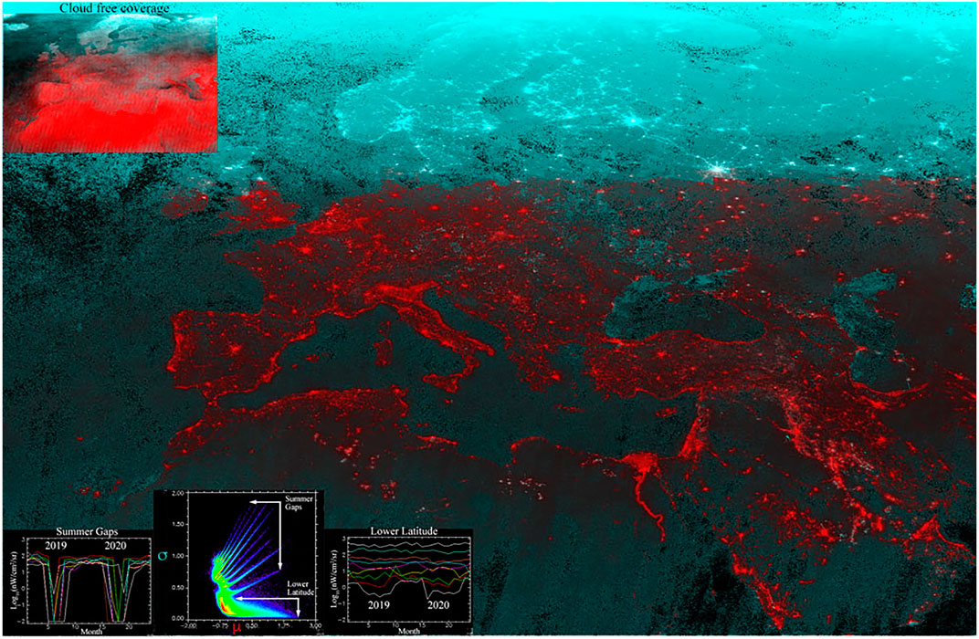
FIGURE 1. (A) Spatiotemporal moments for Log₁₀ VIIRS monthly radiance for 2019 + 2020. Mean (μ) monthly Log₁₀ radiance (red) is consistently high for lighted development and relatively low elsewhere, while the standard deviation (σ) of monthly Log₁₀ radiance (cyan) is low for lighted development and relatively high elsewhere. Lighted development at higher latitudes has high μ and σ so appears white. The μ vs σ distribution (inset scatterplot) shows spurs of rapidly increasing σ with μ for high latitude coverage gaps in summer months. Individual spurs of increasing μ and σ on the upper limb of the scatterplot correspond to brighter sources with different summer gap lengths (inset left). Monotonically decreasing range of σ for μ > 1 nW/cm²/sr on the lowest limb of the distribution results from increasing temporal stability (decreasing σ) with increasing brightness for sources south of the summer gap latitudes (inset right). Gas flares at all latitudes are both bright and variable (white). Inset map of μ and σ for cloud free acquisitions per month for 2019 + 2020 (top) shows a similar pattern as a result of both cloud cover and high latitude coverage gaps.

FIGURE 1

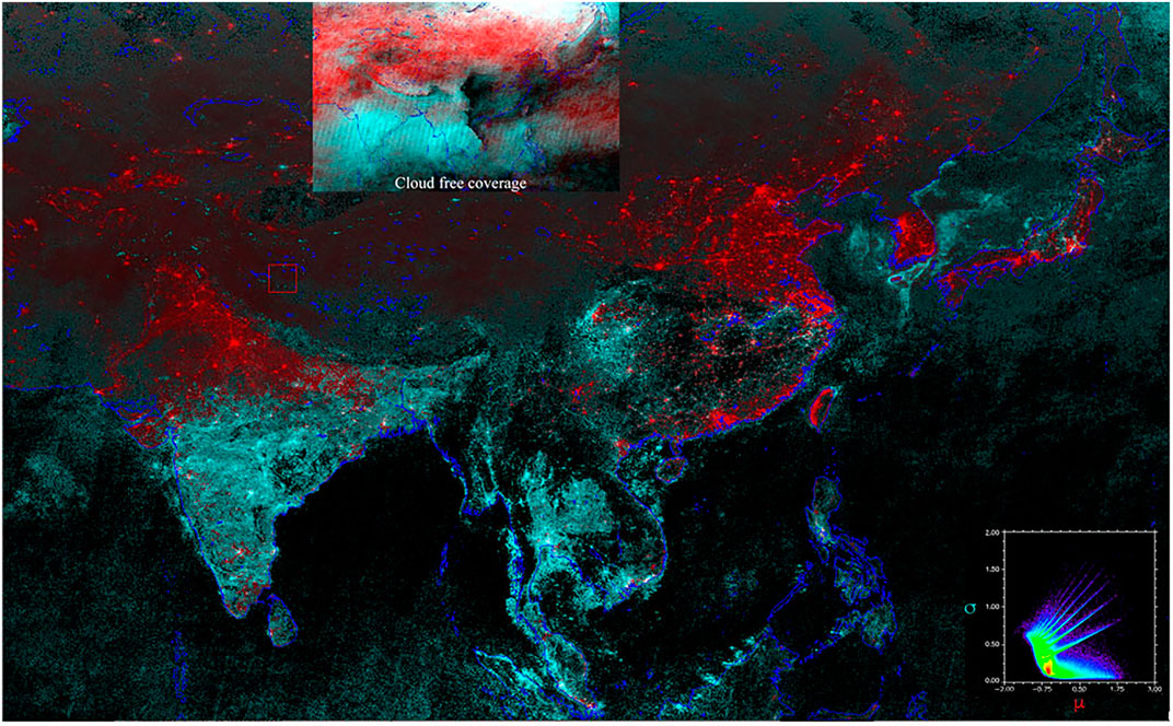
FIGURE 1. (B) Spatiotemporal moments for Log₁₀ VIIRS monthly radiance for Asia in 2019 + 2020. Mean (μ) monthly Log₁₀ radiance (red) is consistently high for lighted development and relatively low elsewhere, while the standard deviation (σ) of monthly Log₁₀ radiance (cyan) is low for lighted development and relatively high elsewhere. Lighted development in summer monsoon areas has high μ and σ so appears white. The μ vs σ distribution (inset scatterplot) shows spurs of rapidly increasing σ with μ for high latitude coverage gaps in summer months. Individual spurs of increasing μ and σ on upper scatterplot correspond to brighter sources with different summer gap lengths (inset left). Monotonically decreasing range of σ for μ > 1 nW/cm2/sr on the lowest limb of the distribution results from increasing temporal stability (decreasing σ) with increasing brightness for sources outside the summer monsoon gap areas (inset right). Inset map of μ and σ for cloud free acquisitions per month for 2019 + 2020(top) shows a similar pattern as a result of monsoon cloud cover.

Spatial correlation matrices of VIIRS monthly mean radiance composites for 2019 + 2020 show correlations between 0.7 and 0.9 for all pairs of months. Heteroskedasticity of the mode of the distributions results from month to month variability in background luminance which reduces the spatial correlation for large numbers of low luminance pixels. Tri-temporal color composites of mean radiance for the months with the three lowest spatial correlations are shown in Figure 2. Areas with similar brightness in all 3 months appear shades of gray. Color implies change. The upper composite shows the anomalously low brightness for large areas of Russia, the Alps and Anatolian plateau in December 2020 as shades of red/orange and a narrow high latitude zone of anomalously high brightness in May 2020 as green along the top of the panel. The lower panel illustrates the effect of seasonal differences. This composite shows the periurban peripheries of lighted developments on the Russian steppe, Alps and Anatolian plateau with higher brightness in January 2020, consistent with the presence of high albedo snow in winter and low albedo vegetation in summer. This is consistent with the seasonality observed by (Levin 2017) and (Levin and Zhang 2017), although it should be noted that this variability is limited to periurban areas with lower luminance–and presumably much larger areas of illuminated snow and vegetation than the brighter urban cores. As with the moment spaces in Figure 1, the inset scatterplots in both panels show strong heteroskedasticity with much greater dispersion at lower brightness levels, diminishing monotonically as brightness increases. It is also noteworthy that the considerable skewness magnitude and polarity of the lower tails of all these bivariate distributions varies among all pairs while the upper tail of each distribution remains symmetric about the 1:1 line.

FIGURE 2

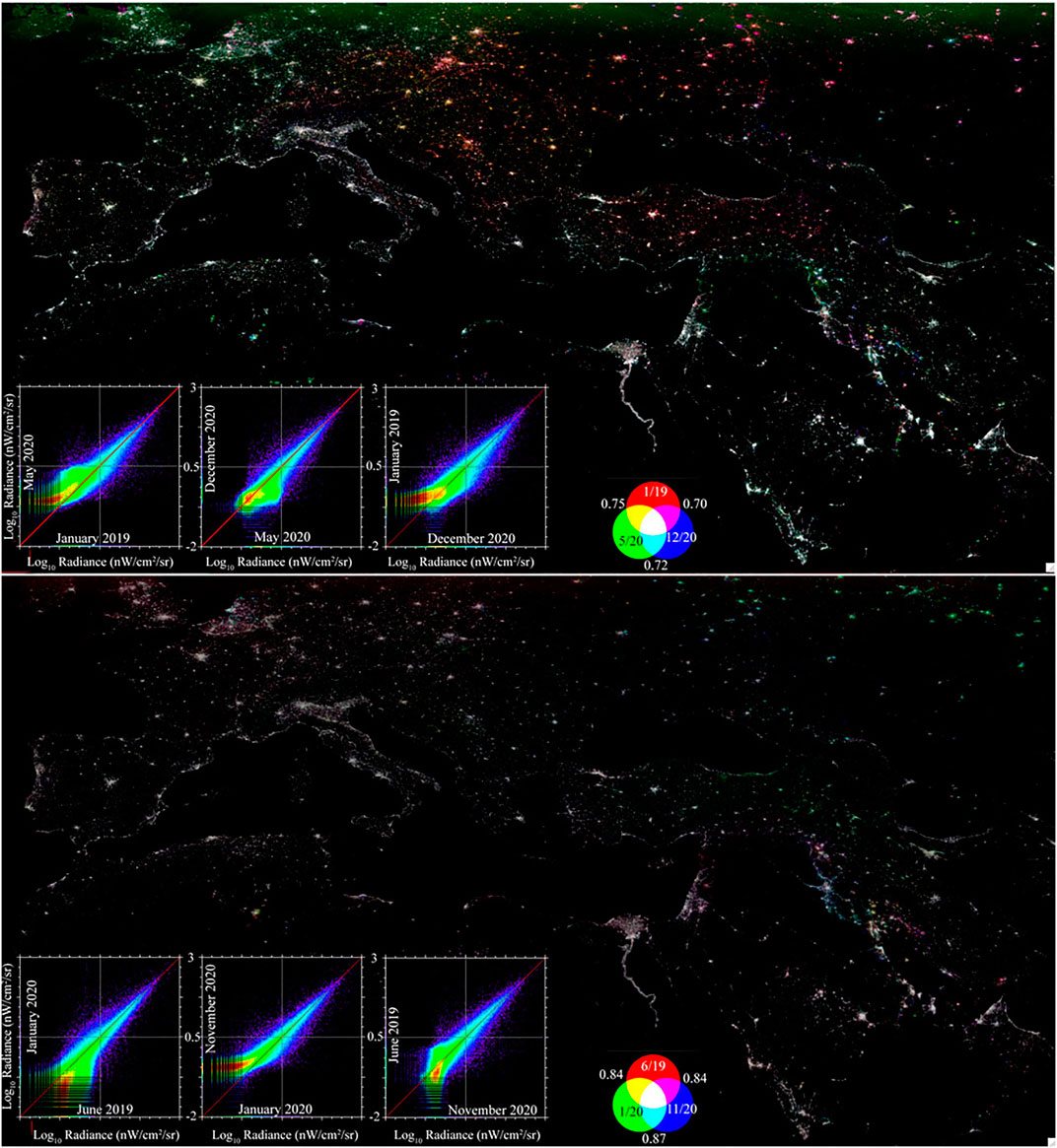
FIGURE 2. Tri-temporal composites of lowest spatial correlation. Color implies change. May 2020 and December 2020 (top) have much lower correlation to all other months (inset RGB). Aside from these two anomalous dates, summer and winter pairs have lower correlations (bottom) than same season pairs, which are generally >0.88. Correlations are computed using only pixels >10^+0.5 nW/cm²/sr to exclude effects of background luminance changes. Note geographic contiguity of change areas.

The seasonal periodicity indicated by the monthly spatial correlation matrix suggests that interannual changes should be most apparent when comparing the same months of different years. Figure 3 shows scatterplots comparing monthly mean radiance for 2019 and 2020 for the Eurasian region shown in Figures 1, 2. As with the subannual comparisons in Figure 2, the interannual bivariate distributions are all strongly heteroskedastic with skewed lower tails and symmetric upper tails. There is no obvious consistency in the month-to-month skewness variations, while the upper tails are consistently symmetric for radiances > 10^0.5 nW/cm²/sr. Similar distributions are observed elsewhere on Earth (Small 2021).

FIGURE 3

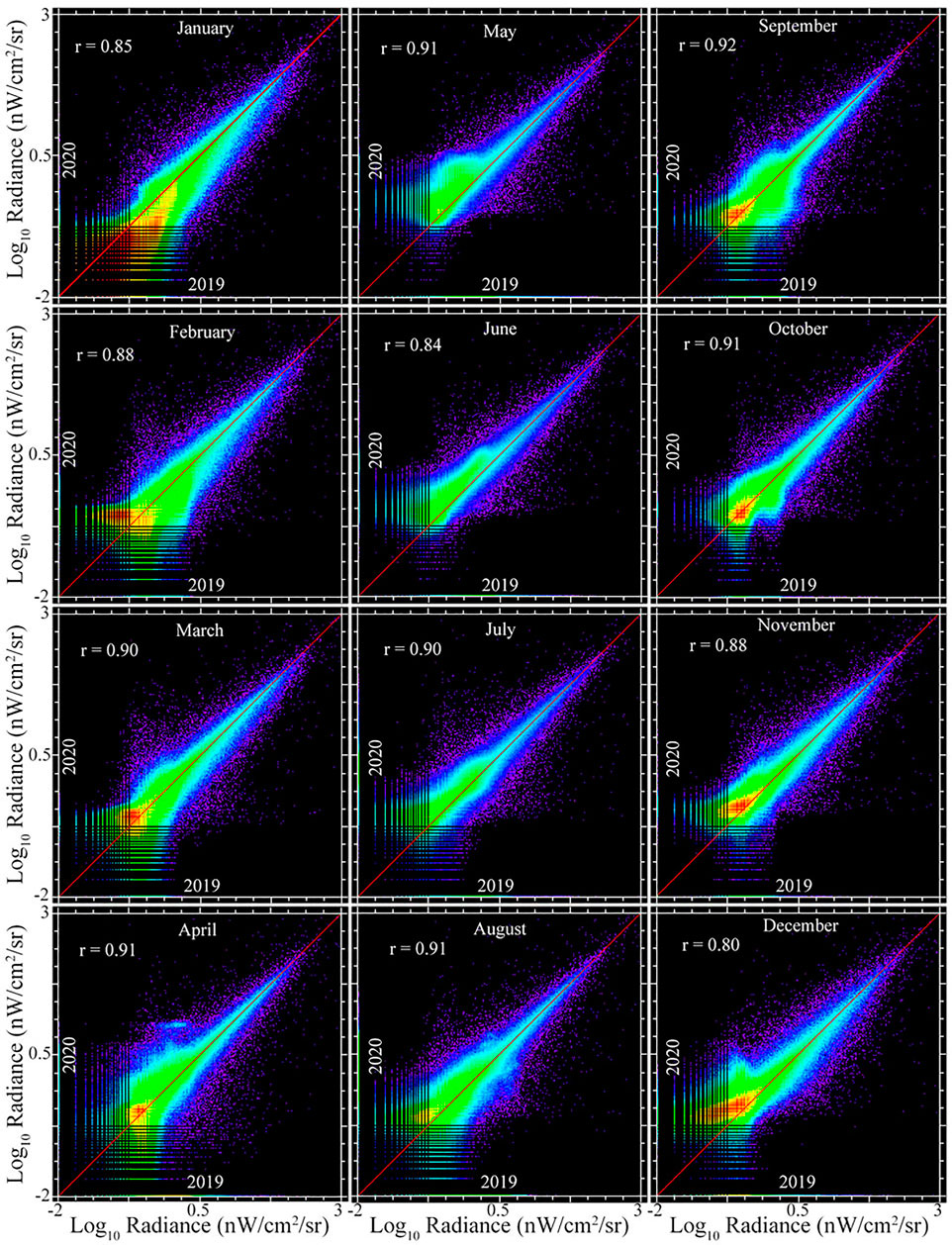
FIGURE 3. Monthly comparisons of 2019 and 2020 for Eurasia. In all months, dispersion about the 1:1 line diminishes with increasing brightness, with no apparent bias above ∼100.5 nW/cm²/sr. At lower brightness levels, there is considerable bias, varying from month to month. Brighter sources show slight bias suggesting dimming from 2019 to 2020 in January and March, but none apparent in other months. Correlations computed using only radiances >10^+0.5 nW/cm²/sr.

The spatial principal components (PCs) of the 24 monthly mean radiance composites from 2019 + 2020 show the spatial distribution of the dominant modes of spatiotemporal variability for Eurasia driven by the contrast between large numbers of low luminance pixels and much smaller numbers of much brighter pixels (Figure 4). Specifically, a strong contrast between the bright stable anthropogenic lights associated with settlements and the high variability of background luminance in non-lighted areas. Again, the strong contrast between higher latitude and mountainous areas where background reflectance changes seasonally, and lower latitude deserts with negligible seasonality of background reflectance is apparent. This contrast is reflected in the bimodal structure of the temporal feature space of PCs one and 2. The structure of the feature space is similar to that of the moment space as the PC1 represents overall brightness varying in space while PC2 represents the dominant mode of temporal variability.

FIGURE 4

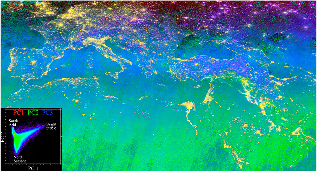
FIGURE 4. Spatial principal components of the 2019 + 2020 monthly time series for Eurasia. PC1, PC2 and PC3 account for 48%, 26% and 6% of spatiotemporal variance (respectively). The temporal feature space (inset) shows PC1 corresponding to overall brightness and temporal stability as PC2 represents latitudinal variations in background luminance. PC3 also shows seasonal variability consistent with persistent winter snow cover in mountainous and steppe regions.

In order to suppress the effects of variance heteroskedasticity on the PC rotation, the 24 months image time series was rotated with all pixel time series with radiances less than 10^0.5 nW/cm²/sr masked. Limiting the rotation parameters to those time series with larger radiances effectively focuses the EOF analysis on the variance of anthropogenic light sources. Figure 5 shows a tri-temporal composite of the three low order PCs from the masked time series. As with the other composites, the effect of background reflectance of land cover is clearly apparent–even though it is limited to the larger periurban areas at the scale of the figure. However, it is also clear that there is much greater variability in most of the urban areas, indicated by a greater variety of colors resulting from varying combinations of the low order EOFs. The inset EOFs show a clear distinction among spatial variations in overall brightness (PC1 – red), seasonal variations (PC2 – green) and interannual variations (PC3 – blue). Note that all 3 PCs have both positive and negative values, implying that each corresponding EOF occurs in both polarities. Hence, the upward trend of EOF3 would correspond to decreases in brightness in pixels with negative PC3 values. The overall variance partition derived from the eigenvalues of the covariance matrix are 88, 2 and 2% for dimensions 1, two and three respectively. This suggests that almost 90% of the spatiotemporal variance is associated with spatial variations in average brightness while 8% of variance is associated with the remaining higher (>3) order modes representing stochastic variability and only 2% each for seasonal and interannual temporal variability. With background luminance suppressed, most anthropogenic night light detected by VIIRS appears to be remarkably stable in at monthly time scales.

FIGURE 5

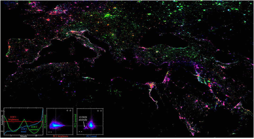
FIGURE 5. PCs, EOFs and temporal feature space for 2019 + 2020 monthly time series for Eurasia with luminance threshold applied. PC1, PC2 and PC3 account for 88, 2 and 2% of spatiotemporal variance (respectively). The >10^+0.5 nW/cm²/sr low luminance threshold eliminates large areas of background luminance so the transformation reflects the spatiotemporal characteristics of the much smaller area of brighter anthropogenic luminance. Bright, temporally stable, urban cores appear red because brightness is modulated by EOF1 and PC1. Magenta and green areas represent variations in the lower luminance periphery where seasonal and interannual changes from residual background luminance approach the contribution of the dimmer anthropogenic light sources. Most of the seasonal (green) areas correspond to mountains or steppe where winter snow and summer vegetation result in higher winter and lower summer albedo. The sign of each PC value determines the polarity of its EOF. The distinct cluster of pixels in quadrant three of PC2-PC3 corresponds to parts of eastern Europe and Russia where December 2020 had anomalously low luminance.

The spectral feature space of the three low order dimensions of the low-luminance masked image time series shown in Figure 6 is consistent with both the temporal moment spaces (Figure 1) and the bivariate brightness distributions (Figure 3). As overall brightness (PC1) increases, both seasonal (PC2) and interannual (PC3) variance decrease monotonically. The inset time series taken from the upper edge of the envelope of PC1/PC2 distribution show considerable month-to-month variability superimposed on the seasonal cycles, consistent with a variance partition between deterministic (PC ≤ 3) and stochastic (PC > 3) variance. The PC3/PC2 space is effectively a phase plane in which different combinations of positive and negative PC weights for EOFs two and three represent different combinations of seasonality and interannual change between 2019 and 2020. Note that the example time series 2 and 4 are not actually monotonic trends as EOF three depicts, but abrupt increases and decreases. This is consistent with the way that abrupt changes are often represented in low order EOFs (Small 2012).

FIGURE 6

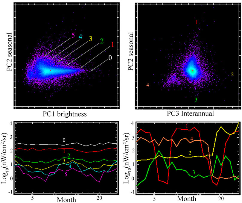
FIGURE 6. Temporal feature space and example time series for 2019 + 2020 monthly mean with luminance threshold applied. Seasonal variability diminishes with increasing brightness (left), Brightness changes significantly greater than month to month variability occur, but are exceedingly rare (right).

Using the spatial PC maps for dimensions 2 and 3 as anomaly detectors makes it possible to immediately identify locations exhibiting strong seasonality or changes between 2019 and 2020. Figures 7–10 show contrasting examples of seasonal changes in 2020 as tri-temporal composites with example time series for individual pixels. Figures 11–13 show examples of interannual changes between 2014, 2017 and 2020 as tri-temporal composites from april of each year. April was chosen to minimize the effects of snow cover at higher latitudes and elevations and the effect of monsoon cloud cover at lower latitudes.

FIGURE 7

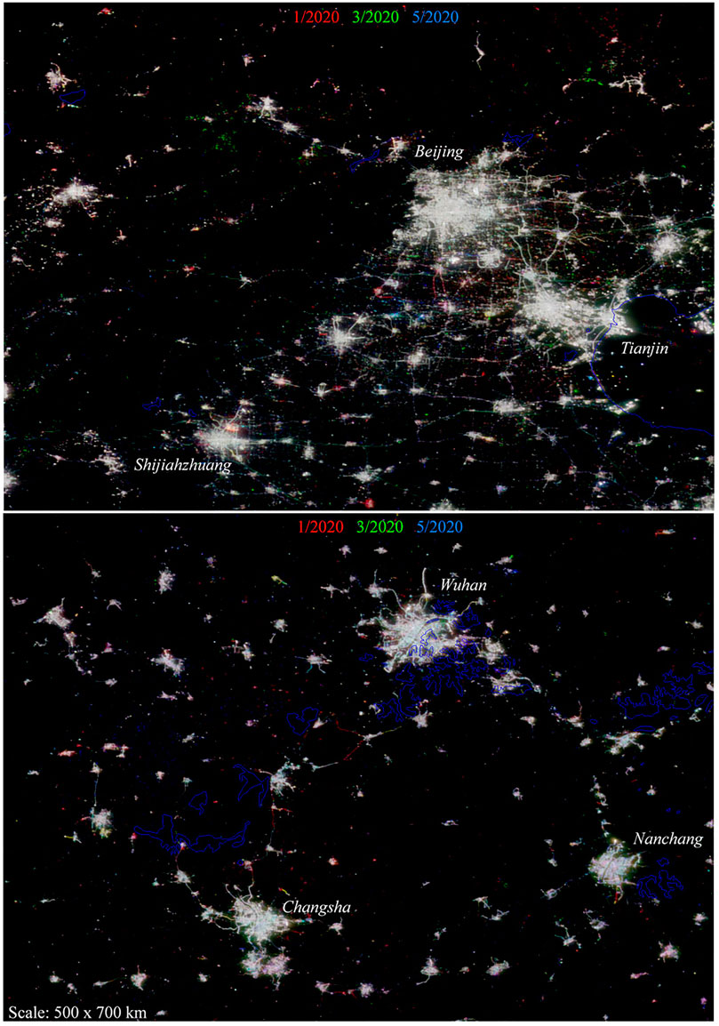
FIGURE 7. Night light stability in China. Tri-temporal composites of monthly mean radiance for early 2020 shows almost all lights as unchanging (shades of gray), with a few small exceptions. No evidence for persistent or widespread reduction in night light during the 2020 lockdowns. Color implies change. Warmer colors imply dimming between January and May 2020.

FIGURE 8

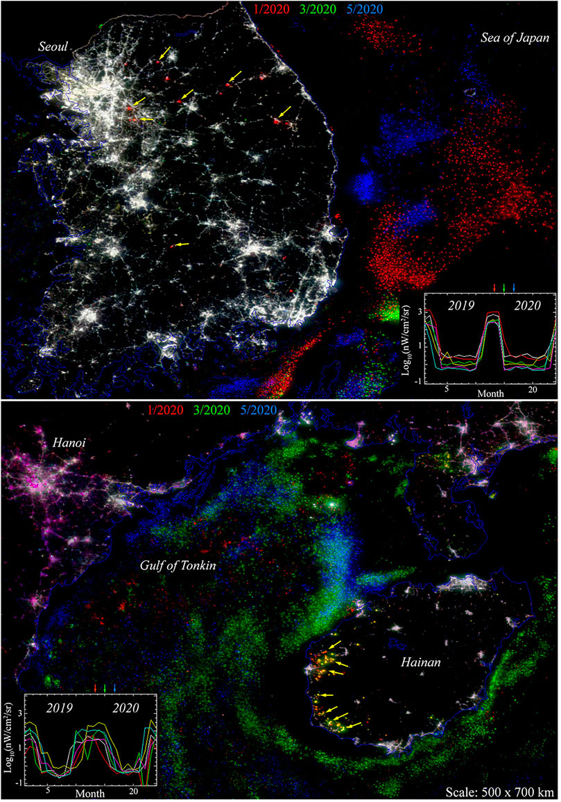
FIGURE 8. Seasonal night light in coastal east Asia. Tri-temporal composites of monthly mean radiance for early 2020 shows most urban lights as unchanging (shades of gray). Color implies change. Warmer colors imply dimming between January and May 2020. Small isolated sites with seasonal fluctuations in northern South Korea and western Hainan Island occur in 2019 and 2020 (arrows and inset plots). More prominent are the seasonal movements of fishing fleets in the Sea of Japan and Gulf of Tonkin. The apparent change in Hanoi and other Red River Delta cities results from cloud cover reduced brightness in March 2020.

FIGURE 9

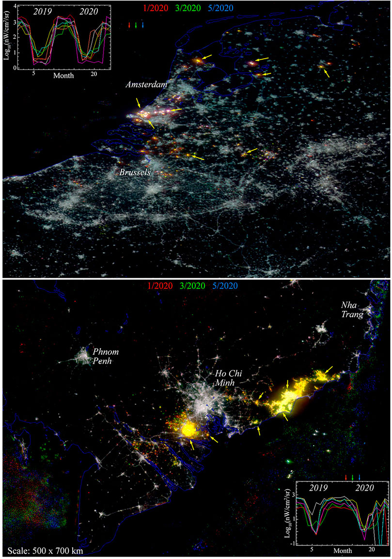
FIGURE 9. Nocturnal horticulture. Tri-temporal composites of monthly mean radiance shows urban lights as unchanging (shades of gray). Color implies change. Warmer colors imply dimming between January and May 2020. Isolated sites of greenhouse clusters in the Netherlands and Belgium (top) and extensive Dragonfruit plantations in southern Vietnam (bottom) are seasonally lighted in 2019 and 2020 (arrows and inset plots).

FIGURE 10

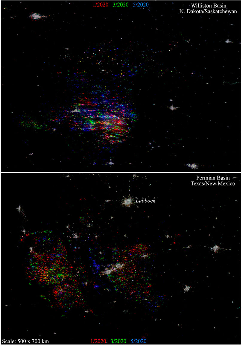
FIGURE 10. Intermittent lights and gas flares from densely spaced hydrofracture wells in North America. Tri-temporal composites of monthly mean radiance for early 2020 shows small urban lights unchanging (shades of gray). Color implies change. Warmer colors imply dimming between January and May 2020.

FIGURE 11

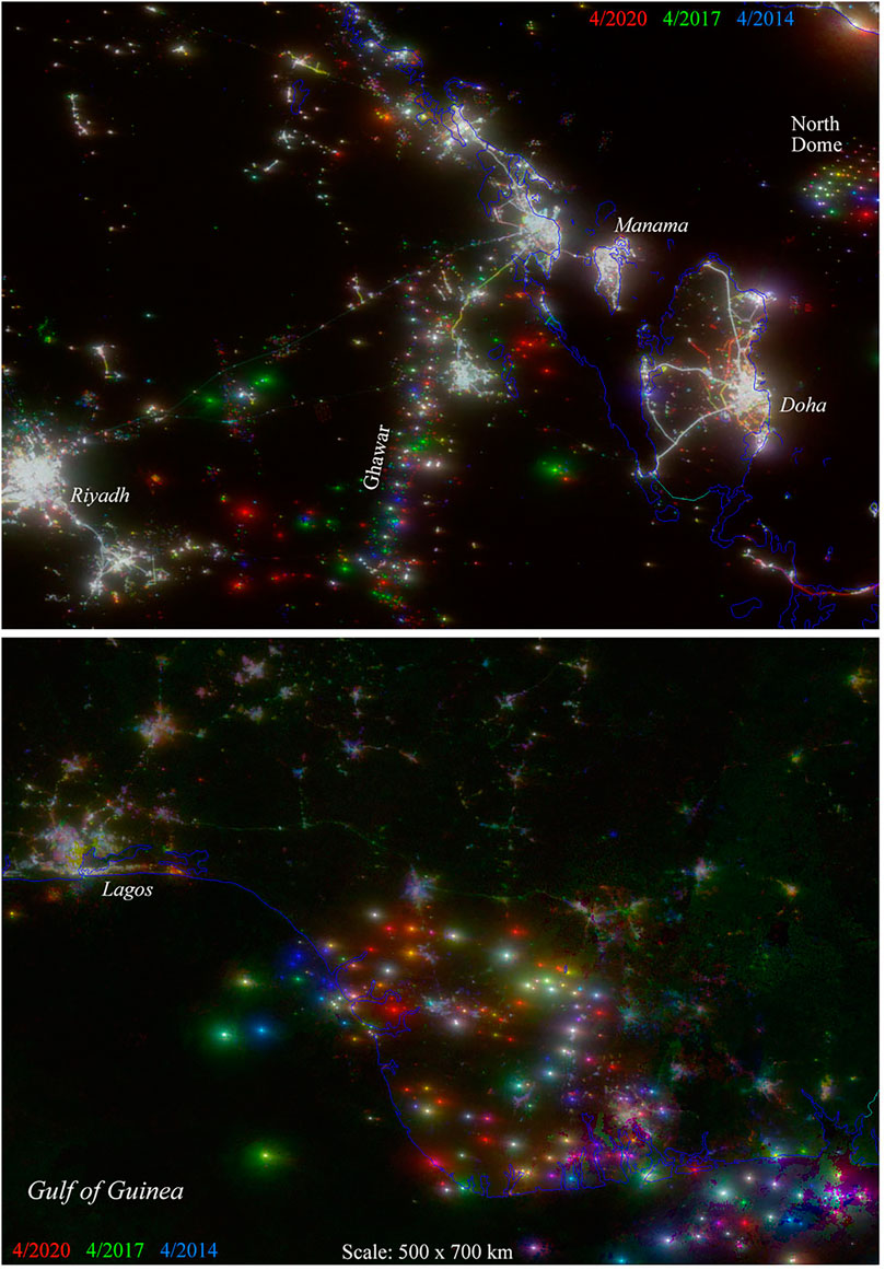
FIGURE 11. Interannual variability of anthropogenic night light associated with oil and gas production. Stable lights appear shades of gray. Color implies change. Northwestern Arabia and the southern Gulf (top) shows pervasive change of production infrastructure lighting on both the Ghawar oilfield onshore and the North Dome gas field offshore. The Niger Delta (bottom) shows more extensive change of both small settlements and oil production. Gas flares are characterized by larger, brighter sources and much larger peripheral halos.

FIGURE 12

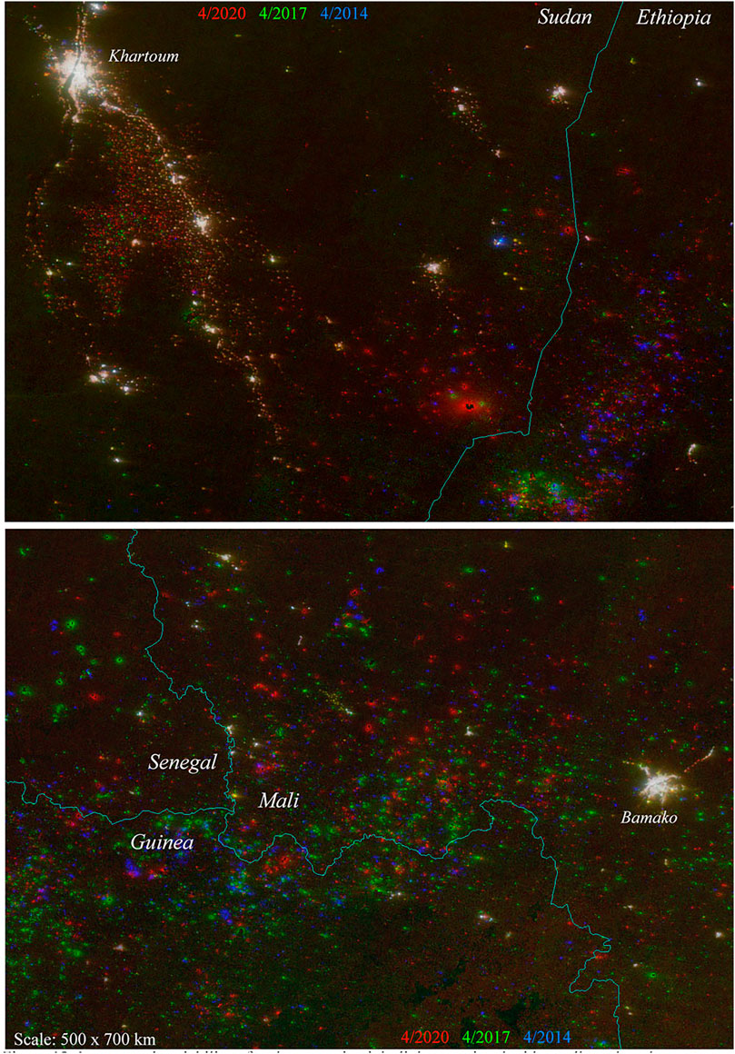
FIGURE 12. Interannual variability of anthropogenic night light associated with small rural settlements in Africa. Stable lights appear shades of gray. Color implies change. Most small sources southeast of Khartoum (top) show progressive brightness increase since 2014 (red), but those in Ethiopia show both sustained increase and decrease (blue). In contrast, numerous small sources in western Africa (bottom) show both sustained increase and increase followed by decrease (green). In the latter case, the decrease post 2017 is partial with 2020 brightness still greater than in 2014.

FIGURE 13

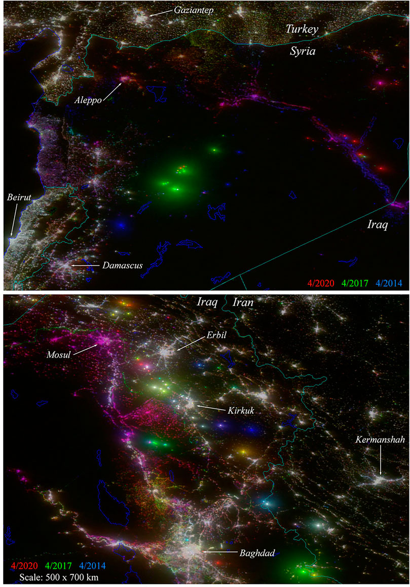
FIGURE 13. Interannual variability of anthropogenic night light associated with conflict. Stable lights appear shades of gray. Color implies change. Bright isolated lights with halos are gas flares. Large area changes of smaller lights likely indicate changes related to power outages at the time of VIIRS′ overpass.

Discussion

Implications of Subannual Variability

A key result of this study is the pervasive heteroskedasticity of VIIRS monthly mean night light. Specifically, the monotonic decrease of temporal variability with increasing mean brightness. Bivariate distributions for all monthly pairs, temporal moment distributions and temporal feature spaces all show this pattern consistently for all years and geographic regions. The three primary sources of geographic temporal variability are latitude-dependent summer gaps in low light acquisitions, summer monsoon cloud cover variations and seasonal changes in background reflectance at higher latitudes and elevations where snow is more persistent in winter and vegetation in summer. However, heteroskedasticity is a pervasive characteristic of the monthly composites and is present in all areas for all months of the year, suggesting that much, if not most, of the month-to-month variability may be related to luminance of otherwise stable sources subjected to multiple aspects of the imaging process varying in time. Three of the most obvious that have been documented are viewing geometry (Li et al., 2019), atmospheric opacity related to aerosols (Fu et al., 2018; Román et al., 2018) and tropospheric water vapor observed frequently in astronaut photos of cities at night (Small 2019).

EOF analysis quantifies the remarkable stability of brighter sources of night light. Specifically, in urban areas and other types of lighted development. While the two dominant forms of deterministic change (EOF2 and EOF3) account for 2% of variance each, spatial variations in brightness account for almost 90% and stochastic variance accounts for almost 10%. EOF analysis also illustrates the pervasive influence of background reflectance in dimly lighted periurban and unlighted rural areas–even with a moderate low luminance threshold (10^+0.5 nW/cm²/sr) used to mask background luminance variations.

Aggregate Metrics of Change

The heteroskedastic nature of monthly night light composites has important implications for studies that infer actual change in light sources from aggregate metrics like Sum of Lights (SoL) and Number of Pixels (NoP). Even studies that apply low luminance thresholds are subject to variability at the level of the threshold. Given the skewed distribution of all night light arising from radial peripheral dimming of bright sources, even aggregate metrics using thresholds must be interpreted in light of the fact that much larger numbers of more variable low luminance pixels may statistically overwhelm smaller numbers of stable higher luminance pixels and cause apparent changes related to the imaging process to be interpreted as actual changes in the light sources. The aggregation process may conceal the most obvious effects of month-to-month variability, but does so at the risk of misattribution of apparent variability to actual change.

Spatiotemporal Anomaly Detection

Because EOF analysis can orthogonalize seasonal and interannual variability as distinct from spatial variability in average brightness, the spatial PCs of these higher dimensions can be used as anomaly detectors to easily identify light sources potentially having undergone actual deterministic change that is statistically distinguishable from both spatial variations in brightness and stochastic temporal variations. As such, it can achieve a stated objective of this study: to provide a basis for distinguishing between actual and apparent change in the sources of anthropogenic night light. Unlike commonly used time series fitting and modeling approaches, EOF analysis is model agnostic and free of the biases inherent in curve fitting. The only assumptions inherent in EOF analysis are that variance corresponds to information and that correlation implies redundancy. Clearly, this is not always the case, but it is often a reasonable assumption. Enough so to justify the use of EOF analysis as a tool for characterization of spatiotemporal variability. In addition, when the combination of variance distribution and EOF interpretability allows for a feasible separation of deterministic and stochastic variance, the resulting partition can inform understanding of both. In the case of significant month-to-month or year-to-year variability inconsistent with the nature of stable night light, this variance partition can provide a basis for projection filtering to more clearly isolate the spatial structure of the temporal changes associated with the temporal processes represented by the low order EOFs (Small 2012; Small and Elvidge 2013).

Data Availability Statement

Publicly available datasets were analyzed in this study. This data can be found here: ;https://payneinstitute.mines.edu/eog/.

Author Contributions

The author confirms being the sole contributor of this work and has approved it for publication.

Funding

This research was supported by the endowment of the Lamont Doherty Earth Observatory of Columbia University.

Conflict of Interest

The author declares that the research was conducted in the absence of any commercial or financial relationships that could be construed as a potential conflict of interest.

Publisher’s Note

All claims expressed in this article are solely those of the authors and do not necessarily represent those of their affiliated organizations, or those of the publisher, the editors and the reviewers. Any product that may be evaluated in this article, or claim that may be made by its manufacturer, is not guaranteed or endorsed by the publisher.

Acknowledgments

The author is grateful to both reviewers for constructive suggestions and to Chris Elvidge for numerous illuminating conversations about the nature of night light and its variability.

References

Bretherton, C. S., Smith, C., and Wallace, J. M. (1992). An Intercomparison of Methods for Finding Coupled Patterns in Climate Data. J. Clim. 5, 541–560. doi:10.1175/1520-0442(1992)005<0541:aiomff>2.0.co;2

CrossRef Full Text | Google Scholar

Cao, C., Shao, X., and Uprety, S. (2013). Detecting Light Outages after Severe Storms Using the S-NPP/VIIRS Day/Night Band Radiances. IEEE Geosci. Remote Sensing Lett. 10 (6), 1582–1586. doi:10.1109/lgrs.2013.2262258

CrossRef Full Text | Google Scholar

Chen, Z., Yu, B., Ta, N., Shi, K., Yang, C., Wang, C., et al. (2019). Delineating Seasonal Relationships between Suomi NPP-VIIRS Nighttime Light and Human Activity across Shanghai, China. IEEE J. Sel. Top. Appl. Earth Observations Remote Sensing 12, 4275–4283. doi:10.1109/jstars.2019.2916323

CrossRef Full Text | Google Scholar

Coesfeld, J., Anderson, S. J., Baugh, K., Elvidge, C. D., Schernthanner, H., and Kyba, C. C. M. (2018). Variation of Individual Location Radiance in VIIRS DNB Monthly Composite Images. Remote Sensing 10, 1964. doi:10.3390/rs10121964

CrossRef Full Text | Google Scholar

Elvidge, C. D., Baugh, K. E., Zhizhin, M., and Hsu, F. C. (2013). Why VIIRS Data Are superior to DMSP for Mapping Nighttime Lights. Pro. Asia-Pac. Adv. Netw. 35, 62. Bangkok Thailand. doi:10.7125/apan.35.7

CrossRef Full Text | Google Scholar

Elvidge, C. D., Baugh, K., Zhizhin, M., Hsu, F. C., and Ghosh, T. (2017). VIIRS Night-Time Lights. Int. J. Remote Sensing 38 (21), 5860–5879. doi:10.1080/01431161.2017.1342050

CrossRef Full Text | Google Scholar

Elvidge, C. D., Zhizhin, M., Baugh, K., Hsu, F.-C., and Ghosh, T. (2016). Methods for Global Survey of Natural Gas Flaring from Visible Infrared Imaging Radiometer Suite Data. Energies 9 (1),14. doi:10.3390/en9010014

CrossRef Full Text | Google Scholar

Elvidge, C., Ziskin, D., Baugh, K., Tuttle, B., Ghosh, T., Pack, D., et al. (2009). A Fifteen Year Record of Global Natural Gas Flaring Derived from Satellite Data. Energies 2 (3), 595–622. doi:10.3390/en20300595

CrossRef Full Text | Google Scholar

Fu, D., Xia, X., Duan, M., Zhang, X., Li, X., Wang, J., et al. (2018). Mapping Nighttime PM2.5 from VIIRS DNB Using a Linear Mixed-Effect Model. Atmos. Environ. 178, 214–222. doi:10.1016/j.atmosenv.2018.02.001

CrossRef Full Text | Google Scholar

Hale, J. D., Davies, G., Fairbrass, A. J., Matthews, T. J., Rogers, C. D., and Sadler, J. P. (2013). Mapping Lightscapes: Spatial Patterning of Artificial Lighting in an Urban Landscape. PLoS One 8 (5), e61460. doi:10.1371/journal.pone.0061460

PubMed Abstract | CrossRef Full Text | Google Scholar

Ji, G., Zhao, J., Yang, X., Yue, Y., and Wang, Z. (2018). Exploring China's 21-year PM10 Emissions Spatiotemporal Variations by DMSP-OLS Nighttime Stable Light Data. Atmos. Environ. 191, 132–141. doi:10.1016/j.atmosenv.2018.07.045

CrossRef Full Text | Google Scholar

Kohiyama, M., Hayashi, H., Maki, N., Higashida, M., Kroehl, H. W., Elvidge, C. D., et al. (2004). Early Damaged Area Estimation System Using DMSP-OLS Night-Time Imagery. Int. J. Remote Sensing 25 (11), 2015–2036. doi:10.1080/01431160310001595033

CrossRef Full Text | Google Scholar

Kuechly, H. U., Kyba, C. C. M., Ruhtz, T., Lindemann, C., Wolter, C., Fischer, J., et al. (2012). Aerial Survey and Spatial Analysis of Sources of Light Pollution in Berlin, Germany. Remote Sensing Environ. 126, 39–50. doi:10.1016/j.rse.2012.08.008

CrossRef Full Text | Google Scholar

Levin, N., Ali, S., and Crandall, D. (2017). Utilizing Remote Sensing and Big Data to Quantify Conflict Intensity: The Arab Spring as a Case Study. Appl. Geogr. 94, 1–17. doi:10.1016/j.apgeog.2018.03.001

CrossRef Full Text | Google Scholar

Levin, N., Johansen, K., Hacker, J. M., and Phinn, S. (2014). A New Source for High Spatial Resolution Night Time Images - the EROS-B Commercial Satellite. Remote Sensing Environ. 149, 1–12. doi:10.1016/j.rse.2014.03.019

CrossRef Full Text | Google Scholar

Levin, N. (2017). The Impact of Seasonal Changes on Observed Nighttime Brightness from 2014 to 2015 Monthly VIIRS DNB Composites. Remote Sensing Environ. 193, 150–164. doi:10.1016/j.rse.2017.03.003

CrossRef Full Text | Google Scholar

Levin, N., and Zhang, Q. (2017). A Global Analysis of Factors Controlling VIIRS Nighttime Light Levels from Densely Populated Areas. Remote Sensing Environ. 190, 366–382. doi:10.1016/j.rse.2017.01.006

CrossRef Full Text | Google Scholar

Li, X., Chen, F., and Chen, X. (2013). Satellite-observed Nighttime Light Variation as Evidence for Global Armed Conflicts. IEEE J. Sel. Top. Appl. Earth Observations Remote Sensing 6 (5), 2302–2315. doi:10.1109/jstars.2013.2241021

CrossRef Full Text | Google Scholar

Li, X., Levin, N., Xie, J., and Li, D. (2020). Monitoring Hourly Night-Time Light by an Unmanned Aerial Vehicle and its Implications to Satellite Remote Sensing. Remote Sensing Environ. 247, 111942. doi:10.1016/j.rse.2020.111942

CrossRef Full Text | Google Scholar

Li, X., and Li, D. (2014). Can Night-Time Light Images Play a Role in Evaluating the Syrian Crisis? Int. J. Remote Sensing 35 (18), 6648–6661. doi:10.1080/01431161.2014.971469

CrossRef Full Text | Google Scholar

Li, X., Liu, S., Jendryke, M., Li, D., and Wu, C. (2018). Night-Time Light Dynamics during the Iraqi Civil War. Remote Sensing 10, 858. doi:10.3390/rs10060858

CrossRef Full Text | Google Scholar

Li, X., Ma, R., Zhang, Q., Li, D., Liu, S., He, T., et al. (2019). Anisotropic Characteristic of Artificial Light at Night - Systematic Investigation with VIIRS DNB Multi-Temporal Observations. Remote Sensing Environ. 233, 111357. doi:10.1016/j.rse.2019.111357

CrossRef Full Text | Google Scholar

Lorenz, E. N. (1956). Empirical Orthogonal Functions and Statistical Weather Prediction. Statistical Forecasting Project (Cambridge, MA: MIT), 48.

Google Scholar

Mann, M. L., Melaas, E. K., and Malik, A. (2016). Using VIIRS Day/Night Band to Measure Electricity Supply Reliability: Preliminary Results from Maharashtra, India. Remote Sensing 8 (9), 711. doi:10.3390/rs8090711

CrossRef Full Text | Google Scholar

Miller, S., Straka, W., Mills, S., Elvidge, C., Lee, T., Solbrig, J., et al. (2013). Illuminating the Capabilities of the Suomi National Polar-Orbiting Partnership (NPP) Visible Infrared Imaging Radiometer Suite (VIIRS) Day/Night Band. Remote Sensing 5, 6717–6766. doi:10.3390/rs5126717

CrossRef Full Text | Google Scholar

Preisendorfer, R. W. (1988). Principal Component Analysis in Meteorology and Oceanography. Amsterdam: Elsevier.

Google Scholar

Roman, M. O., and Stokes, E. C. (2015). Holidays in Lights: Tracking Cultural Patterns in Demand for Energy Services. Earth’s Future 3, 182. doi:10.1002/2014ef000285

CrossRef Full Text | Google Scholar

Román, M. O., Wang, Z., Sun, Q., Kalb, V., Miller, S. D., Molthan, A., et al. (2018). NASA's Black Marble Nighttime Lights Product Suite. Remote Sensing Environ. 210, 113–143. doi:10.1016/j.rse.2018.03.017

CrossRef Full Text | Google Scholar

Small, C., and Elvidge, C. D. (2013). Night on Earth: Mapping Decadal Changes of Anthropogenic Night Light in Asia. Int. J. Appl. Earth Observation Geoinformation 22 (1), 40–52. doi:10.1016/j.jag.2012.02.009

CrossRef Full Text | Google Scholar

Small, C. (2019). Multisensor Characterization of Urban Morphology and Network Structure. Remote Sensing 11 (2162), 1–30. doi:10.3390/rs11182162

CrossRef Full Text | Google Scholar

Small, C. (2021). Spatiotemporal Characterization of VIIRS Night Light. ArXiv. Available at: https://arxiv.org/abs/2109.06913 (Accessed November 24, 2021).

CrossRef Full Text | Google Scholar

Small, C. (2012). Spatiotemporal Dimensionality and Time-Space Characterization of Multitemporal Imagery. Remote Sensing Environ. 124, 793–809. doi:10.1016/j.rse.2012.05.031

CrossRef Full Text | Google Scholar

von_Storch, H., and Zwiers, F. W. (1999). Statistical Analysis in Climate Research. Cambridge UK: Cambridge University Press.

Google Scholar

Zeng, X., Shao, X., Qiu, S., Ma, L., Gao, C., and Li, C. (2018). Stability Monitoring of the VIIRS Day/Night Band over Dome C with a Lunar Irradiance Model and BRDF Correction. Remote Sensing 10 (2), 189. doi:10.3390/rs10020189

CrossRef Full Text | Google Scholar

Zhang, X., Scheving, B., Shoghli, B., Zygarlicke, C., and Wocken, C. (2015). Quantifying Gas Flaring CH4 Consumption Using VIIRS. Remote Sensing 7 (8), 9529. doi:10.3390/rs70809529

CrossRef Full Text | Google Scholar