Earth Polychromatic Imaging Camera Geolocation; Strategies to Reduce Uncertainty

Earth Polychromatic Imaging Camera occupies a unique point of view for an Earth imager by being located approximately 1.5 million km from the planet at Earth-Sun Lagrange point, L1. This creates a number of unique challenges in geolocation, some of which are distance and mission specific. To solve these problems, algorithmic adaptations need to be made for calculations used for standard geolocation solutions, as well as artificial intelligence-based corrections for star tracker attitude and optical issues. This paper discusses methods for resolving these issues and bringing the geolocation solution to within requirements.

Introduction

Instrument

The Earth Polychromatic Imaging Camera (EPIC) is an instrument on the Deep Space Climate Observatory (DSCOVR), which orbits the L1 Earth-Sun Lagrange point. As an Earth viewing instrument, it has a unique view of the planet, taking 13–21 images daily at local noon. The instrument is a 30 cm Cassegrain telescope with 2048x2048 charge-coupled device (CCD), using two filter wheels, and containing a set of 10 bands at wavelengths between 317 and 780 nm (Figure 1) (DSCOVR:EPIC, 2016).

FIGURE 1

FIGURE 1. Images of the Earth taken in different wavelength by EPIC. The leftmost panel are infrared bands; middle are visible; right are ultraviolet. The range permits EPIC to engage in land, cloud, and atmospheric studies as well as produce color images.

A typical imaging session consists of 10 images taken once of each band. In creating the science products, the images are calibrated into units of counts/second and then geolocation is calculated (Marshak et al., 2018).

Geolocation

Geolocation for EPIC images is unique because it not only has to operate across the entire illuminated Earth’s surface, but also has to do so from a 1.5 million kilometers away. The algorithm creates ancillary science products per pixel, of the latitude and longitude; Sun azimuth and zenith angles; viewing azimuth and zenith angles; and viewing angle deltas due to Earth atmosphere refraction. For the level 1a (L1a) product, these values are calculated per pixel and mapped into the original image’s orientation. In the level 1b (L1b), the images and the relative products are remapped, so that north is pointed up and the pixels across the bands are aligned with each other. Bands within the visual range are combined to produce natural color images (Figure 2) of the rotation Earth (https://epic.gsfc.nasa.gov).

FIGURE 2

FIGURE 2. Examples of EPIC geolocation products.

It takes about 7 minutes for EPIC to take a set of ten exposures in an imaging session. While the instrument is performing this action, there are several articles of motion occurring. First, the spacecraft is moving, traveling its 6-months Lissajous orbit, rotating on its axis, and making externally driven linear motions to adjust its pointing so that Earth is centered in the view (Figure 3). Second, the subject of the imaging, typically Earth, is rotating on its axis 15° per hour, resulting in approximately a 4-pixel rotational offset between the first and final image in the set.

FIGURE 3

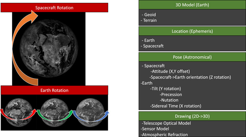
FIGURE 3. Different corrections made by the EPIC geolocation software and the inputs needed for the different parts of the program.

In order to geolocate these images, it is necessary to develop a three-dimensional model of each pixel location. A useful model of the Earth’s body is generated based on the SRTM30 dataset (Shuttle Radar Topography Mission) and rotated into EPIC’s view using spacecraft attitude and ephemeris information, as well as astronomical calculations of the seasonal Earth’s position. This is then lined up with the actual EPIC images and permits the calculation of the latitude, longitude, and relevant Sun and viewing angles. The results of this product are then written into the L1a dataset. In order to generate the L1b, using the 3D coordinates, the pixels for all 10 bands are “spun” into the same orientation, redrawn in 2D, and written into a shared latitude and longitude grid.

More details, as well as a mathematical description of the algorithm can be found in the “EPIC Geolocation and Color Imagery” document (Blank, 2019) found in the references.

Problems

Although the geolocation seems straightforward, there are several challenges that prevent an uncomplicated implementation of this algorithm. The first is that the accuracy of the star tracker is below what is needed to understand the orientation of the instrument and Earths’ body; the second is linked to problems with the optical distortion model of the EPIC telescope; the third is a potential issue with time stamp accuracy.

Star Tracker and Guidance

The star tracker, a Ball Aerospace CT633, contains an imager that looks at stars in the dark sky and matches the resulting star images against its star catalog (Ball, 2021). Using this information, it is able to obtain the attitude of the spacecraft relative to the Earth’s ecliptic plane. From there, with the ephemeris of the Earth and Sun, it is possible to determine how the spacecraft is oriented regarding Earth. If this information was within requirements, it would be possible to calculate directly the per pixel values for the geolocation.

Unfortunately, it is not perfect, an issue that was known when the spacecraft was initially developed as “Triana” in 1999. At that time, engineers had developed a software solution to help mitigate this issue, using images from EPIC to help reorient the spacecraft regarding Earth. But in 2010, when the spacecraft was recommissioned and renamed DSCOVR, its focus transitioned from an Earth science to a space weather mission. EPIC went from the primary instrument to secondary and the EPIC Earth-orienting software was removed. As a result, without the additional correction, the nominally 0.5° Earth images can be anywhere within the field of view.

The accuracy of the star tracker attitude is not adequate for geolocation of the EPIC images. It can be as much as ±0.05° on the x, y offset and ±1° in rotation.

Time

Because the net error in the geolocation was across multiple dimensions, it was difficult to identify exactly the source of all the errors. One potential issue was that the time stamp in the images was not sufficiently accurate. The EPIC images are sensitive to time within a 30 s resolution, but it takes approximately 90 s to go through the process of taking an image. This process includes moving the filter wheel, taking the exposure, processing the image and storing it into memory. The timestamp must also be copied from multiple systems, from the spacecraft to the instrument computer; it adds up to the potential for the appended timestamp to not match the actual exposure time. This would translate to an X axis rotation error in rotating the Earth into the EPIC view. This source of error was investigated and resolved as part of this work.

Optical Distortion

After an initial implementation of the EPIC Geolocation, it became evident there were problems with the optical distortion model of the telescope. This model accounts for both radial and tangential distortion common to lenses. An example of it is to photograph a rectangular grid and view the results. A wide-angle lens with have barrel distortion; a telephoto lens, such as EPIC, will have a pincushion distortion (Figure 4).

FIGURE 4

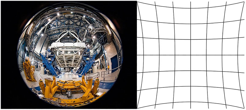
FIGURE 4. Left: Image taken with wide angle lens demonstrating barrel distortion. Credit ESO/José Francisco Salgado. Right: Grid demonstrating pincushion distortion. Credit: Wikipedia/WolfWings.

The formula used for repairing optical distortion is as follows:

Calculate the delta between the physical CCD center and the optical center:

$\Delta x=x-x_c$

$\Delta y=y-y_c$

Radial distance:

$r=\sqrt{\Delta x^2+\Delta y^2}$

The pixel offset, according to the optical model, is then:

$x^{\text{'}}=\Delta x+\left(K_1{r}^2+K_2{r}^4+K_3{r}^6\right)+P_1\left(r^2+2\Delta x^2\right)+2P_2\left(\Delta x\Delta y\right)\left(1+P_3{r}^2+P_4{r}^4\right)$

$y^{\text{'}}=\Delta y+\left(K_1{r}^2+K_2{r}^4+K_3{r}^6\right)+2P_1\left(\Delta x\Delta y\right)+P_2\left(r^2+2\Delta y^2\right)\left(1+P_3{r}^2+P_4{r}^4\right)$

The parts $\left(K_1{r}^2+K_2{r}^4+K_3{r}^6\right)$ and $(1+P_3{r}^2+P_4{r}^4)$ above are infinite expansions in the original formula; here shown are only the terms needed to correct for EPIC where the K’s and the P’s are the parameters that are derived from the optical model.

When comparing results and performing offset analysis, it appeared that there was an error bias that started from the middle of the CCD to the bottom right corner.

Typical Solutions for Geolocation Error

A typical solution to solving geolocation errors is to find control points and warp the images to fit. This was done with success in corrections to early versions of the geolocated product such as used for the algorithm. Here, the data was control point matched and regridded into a new projection. Although this solution worked well for the MAIAC algorithm, it would not make a universal solution for all EPIC science algorithms. Because DSCOVR is constantly in motion as each band is being taken, each image has a unique geolocation solution and therefore a unique set of errors. Some science products, such as ozone, are very sensitive to the band’s colocation. Using warping risks introducing artifacts into these datasets.

Another solution was to use control points and develop a solution to the rotational and x, y linear offsets in the image. Although this could resolve these errors to some degree, it cannot fix problems at far viewing angles of the Earth images or the optical distortion error. This is due to a loss of contrast at higher viewing angles because of atmospheric scattering, as well as a decrease of spatial resolution in the data cause by the Earth’s curvature. Although at 2048 × 2048 the nadir image resolution (point spread function) is 18km, by 70° viewing angle it has degraded to approximately 18km/cost (70°) per pixel, which is 53 km resolution.

Summary of Functions to Be Solved

To resolve the problems with geolocation requires finding a solution for the 16 inputs to the algorithm that are below requirements. These include:

x offset–Earth’s x location from the center of the image.

y offset–Earth’s y location from the center of the image.

Z Earth/DSCOVR rotational offset.

X Earth time rotational offset

plus 13 coefficients in the optical distortion model, including linear offset, radial distortion, and tangential distortion.

The x, y, and rotational offset corrections need will need to be calculated for every image; the optical distortion model only needs to be resolved once. The computational complexity of resolving such a problem with brute force is O (n), where n is the range of error from the computed result. Multi-Angle Implementation of Atmospheric Correction (MAIAC) algorithm (Huang, 2019).

Methods

To reduce the massive problem required the implementation of an EPIC simulator and an artificial intelligence (AI) program. The EPIC simulator is used to generate images of the Earth in different configurations. The AI is used to select potential matches between the simulated images and the actual EPIC picture and determine which solutions are worthwhile to explore.

Earth Polychromatic Imaging Camera Simulator

The EPIC simulator consists of an astronomical calculator, an Earth model, an instrument model, and MODIS (Moderate Resolution Imaging Spectroradiometer) data (Figure 5). It is very similar, and shares much of the code used for EPIC geolocation but is used instead to generate MODIS images simulated to look like EPIC images. The simulator works with any geolocated dataset and has been also tested with VIIRS, GOES-16, and Himawari-8 (see Acronyms for definitions). It can also take EPIC images from another band or time period and convert it into another point of view.

FIGURE 5

FIGURE 5. MODIS full day image in equirectangular projection. From https://worldview.earthdata.nasa.gov/.

FIGURE 6

FIGURE 6. Diagram demonstrating back propagation correction for the EPIC Geolocation.

The astronomical calculator takes the date and time, and calculates the apparent sidereal time, obliquity, precession, nutation, and annual aberration. This determines the “pose” of the Earth at the time the image is taken.

To determine the pose in relation to the camera view angle, the Sun and Spacecraft ephemeris, along with the spacecraft attitude quaternions, are used to calculate the viewing angles.

Using a terrain model of the Earth, the geoid, a 3D model of the Earth is generated in Cartesian coordinates. Then, with the astronomical pose and camera viewing angles, the 3D model is “spun” into the pose it would be in as viewed from the spacecraft. The set of Cartesian coordinates is then clipped so that only those seen by the spacecraft are in the model, and the ones on the far side (not imaged) of the Earth are removed.

Using the telescope optical model, the Cartesian coordinates are mapped into the 2D coordinates of the detector array. MODIS RGB data obtained from WorldView Web Mapping Service (https://worldview.earthdata.nasa.gov/) is then redrawn with the 2D coordinates. The result is a MODIS image that has been reprojected into the EPIC point of view.

Using this simulator, it is possible to generate images to test the instrument’s various configurations. Anything that is input into the geolocation algorithm can be modified to determine how it would affect the resulting image. This can be used to resolve the errors in attitude and optical distortion.

Back Propagation

After the simulator, the next step is to automate the correction process. This is done in a way similar to back propagation (BP) in neural networks.

In this situation, each input to the geolocation is treated as a node; the link between them is the calculation. Each coefficient is initially fed the naïve solution for the input.

The program then generates a coarse spread of potential values. The range of these values is based on the known error range of the inputs. Using this coarse spread, possible configurations of attitude and optical model are fed to the simulator generating dozens of low-resolution Earths. These Earth images are then scored against the actual EPIC image; the coefficients that generated the best match are then propagated back into the algorithm.

The algorithm repeats, but this time with the updated coefficients in the nodes. Another spread is generated, this time at a finer resolution than before. Dozens of Earths are simulated in different configurations, this time at a medium resolution. The simulated earths are then scored, using the Pearson correlation calculation, against the actual EPIC image and the winner is then used to update the coefficients.

The algorithm is run repeatedly, each time at a finer resolution, until it has resolved all the coefficients to meet the geolocation requirements of results within 0.5 pixels. Essentially, what happens is the AI is teaching itself how to draw Earth images so they look like EPIC images; as a result, we learn the necessary coefficients for the geolocation.

When the AI is done, the naïve geolocation algorithm is then run with the updated coefficients and generates the subsequent level 1 products.

Use in Solving Star Tracker

The star tracker attitude solution is necessary for three inputs into the model; the horizontal (y) and vertical (x) offsets of the centroid in the image, and the rotation required to make Earth’s north face the top of the image. The star tracker x and y offsets have never been used in the naïve algorithm, as the error was too great: instead, a centroiding algorithm was used to find the edge of the Earth and center based on that. This algorithm, however, could not always center the Earth within half-a-pixel requirements. This was due partially because the atmosphere makes the edges unsharp. The other reason is because DSCOVR’s orbit is slightly off the Earth-Sun line, so the Sun terminator line is contained in all the images. This means that on one side of the Earth, the edge is always darker and less distinct, and that the location of the terminator is orbit dependent and moves accordingly.

Because of the lack of sharpness of the land in the images due to the atmosphere, and because some images, such as the UV bands, lack distinct surface features, it is necessary to use as much intelligence from the images as possible. By using the EPIC-simulating MODIS images, cloud features, as well as interior land features, can be used to assist the correction.

As there are 10 bands in EPIC, the best band available is used with the simulator; every other band uses EPIC data. The preferred band to use is 780 nm as it has the maximum contrast. If that is not available, then it will choose, in order of preference, 680, 551, 443, 388, 340, 325, 317, 764, and 688 nm. The order is based on the relative correlation scores of these bands to the MODIS image.

The initial back propagation generates a three-value coarse spread for each of the coefficients. For the x and y offsets, this starts at eight pixels, the worst possible error, and for the rotation it starts at 1°. Nine Earths are simulated, scored, and the best result is then put back into the propagation algorithm. This is repeated with each round doubling the precision in resolution until the algorithm reaches the equivalent of 0.25-pixel accuracy.

Use in Solving Time

The method for the time coefficient was the same as that for the star tracker and was calculated alongside those coefficients in earlier tests. It was found that there was no significant error in the image time stamp, and adjustment for this coefficient was subsequently removed.

Use in Solving Optical Distortion

In order to solve the coefficients for optical distortion, the back-propagation (BP) algorithm needs to be used to solve the rotation error to the best of its ability, followed by then applying the BP algorithm to the optical distortion formula. Because we lack ideal images for solving optical distortion, it is necessary to perform the BP correction for optical distortion hundreds of times and collate the results. An ideal image would be a gridded surface that covers the entire field of view–unfortunately that doesn’t exist from the point of view of L1. An alternative would be using a star field image. However, EPIC is not suited for imaging stars, as the filters limit the amount of light such that the exposure would be longer than the spacecraft can stay still. We did attempt to image the stars without the filters, however we found that without the refractive index supplied by the filters, the star images were out of focus.

Using images of the Earth has its own challenges. The optical distortion benefits most from information near the edges of the CCD. However, EPIC images have low data content at the edges, due to the Earth tending to be centered. Furthermore, because of atmospheric haze and distance distortion, the sharpness of the land mass decreases as the viewing angle increases, which means that there is less useful information as you get closer to the edge of the sphere. This is less of a problem with the infrared 780 nm band than the other bands; therefore, we limit the use to this band alone.

Due to these issues, the back propagation does not perform optimally; therefore, it is necessary to run it multiple times on different images and aggregate the results. To reduce the amount of computation required, a program was written to scan through the available EPIC images and pick only best suited for this application. In this situation, we take advantage of the noisy pointing from the star tracker and select images where the Earth is situated closer to the edges of the CCD. To avoid any seasonal or orbital biases, the images were further down selected to be dispersed somewhat evenly, timewise, over the course of 2 years.

The BP algorithm was then run with the attitude and optical distortion correction across approximately 350 images. Outliers selected based on the optical center coordinates were removed. The datasets were then broken into a 2016 and 2017 set, the results then collated by averaging the coefficient values. The 2016 and 2017 coefficient sets were found to be almost identical, which was a good indication that the process could produce consistent results. They were then collected together into a final model. Since the run of this model in 2018, there has been no evidence of drift in the geolocation solution, which indicates the distortion is stable. Because of this, and the fact that this calculation is resource intensive in both computation and in user time, it has not been rerun since then.

Example Run

In the following example run to resolve the star tracker error, the software was run for seven iterations with gradually finer resolutions. The graphs in Figures 7, 8 show the delta between each run and the final solution. In the star tracker this is for the x and y centroid offsets and the rotation to north angle. As can be seen, after the initial coarse calculation, the results rapidly converge and approach the solution (Figures 7, 8).

FIGURE 7

FIGURE 7. Chart demonstrates the software converging on the solution of the x and y centroid offsets as the resolution of each pass increases.

FIGURE 8

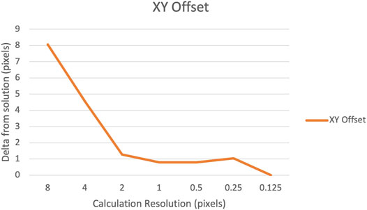
FIGURE 8. Chart demonstrates the software converging on the solution of the rotational correction as each pass increases in resolution.

Below (Figure 9) is an example of the final simulated image using MODIS data and the calculated solution, versus the original EPIC image.

FIGURE 9

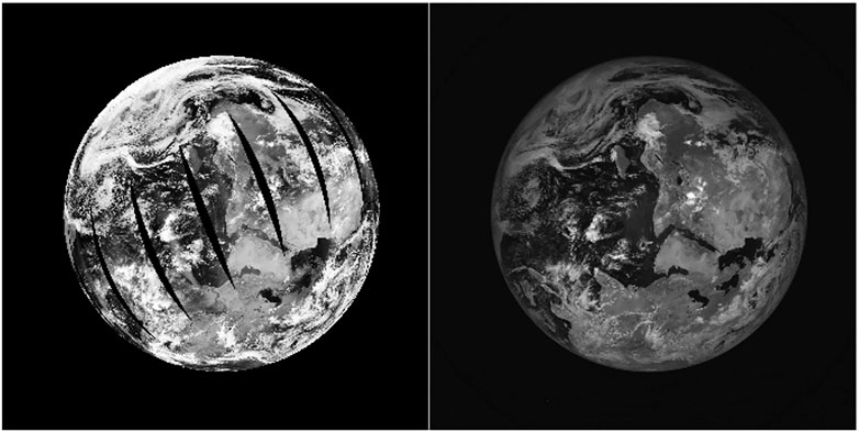
FIGURE 9. Left: MODIS data simulated as EPIC portraying the final solution of the algorithm. Right: Actual EPIC image the algorithm was performed against.

Results

Optical Distortion Solution

The results of the optical distortion solution revealed a severe tangential distortion. Tangential distortion is caused by a skewing of the optical system. The likely result of this is a lift of several millimeters of the CCD at the lower right corner. It is difficult to ascertain when exactly this happened but based on reviews of work orders performed on the reassembly of the instrument, as well as due to some other issues witnessed with the CCD not seen during ground testing, the probability is that it happened during launch.

The improved optical distortion model resolves this issue.

On the left (Figure 10) is the theoretical ideal optical distortion model, which is likely what was intended by the optical designers. This contains only the radial distortion part of the model. On the right is the actual model with both the tangential and radial distortion.

FIGURE 10

FIGURE 10. Left: Optical distortion solution, radial component only. Right: Optical distortion solution, radial and tangential components. The color indicates magnitude of offset due to distortion in pixels.

Star Tracker + Optical Distortion Solution

The back-propagation algorithm resolved the star tracker issue. Prior to this solution, results could be off, in the worst case, by as much as eight pixels. Results are now within 1-pixel accuracy within 70° viewing angle. It may be better than that but results higher than 70° are difficult to judge; the pixel resolution decreases to 53 km per pixel and the reduction in contrast because of atmospheric scattering makes land less visible.

Below (Figure 11) is an example of the final results including both the star tracker and optical distortion solution. On the left is the original solution with the naïve algorithm, on the right, the improved solution.

FIGURE 11

FIGURE 11. Left: Original, naïve geolocation solution. Right: Improved geolocation solution with back propagation.

Conclusion

The AI enhanced BP method resolved the accuracy with the EPIC geolocation due to precision issues with the star tracker attitude and optical distortion model. It can potentially be used on other instruments and missions to resolve accuracy issues due to error in the inputs, as well as resolve calibration issues. It provides an alternative to traditional warping and transformation methods and provides a solution free from distortion.

It can also potentially be used for identifying ambiguous or complex errors, as well as certifying that an input meets requirements.

Data Availability Statement

Publicly available datasets were analyzed in this study. This data can be found here: https://search.earthdata.nasa.gov/.

Author Contributions

KB designed the solutions discussed, wrote the software and the majority of the paper. L-KH, JH, AM were involved in validation of technique and identifying issues that needed to be resolved. All authors contributed to manuscript revision, read, and approved the submitted version.

Funding

Resources supporting this work were provided by the NASA High-End Computing (HEC) Program through the NASA Center for Climate Simulation (NCCS) at Goddard Space Flight Center.

Conflict of Interest

L-KH was employed by Science Systems and Applications, Inc.

The remaining authors declare that the research was conducted in the absence of any commercial or financial relationships that could be construed as a potential conflict of interest.

Publisher’s Note

All claims expressed in this article are solely those of the authors and do not necessarily represent those of their affiliated organizations, or those of the publisher, the editors and the reviewers. Any product that may be evaluated in this article, or claim that may be made by its manufacturer, is not guaranteed or endorsed by the publisher.

Abbreviations

AI, artificial intelligence; BP, back propagation; CCD, charge-couple device; DSCOVR, deep space climate observatory; EPIC, earth polychromatic imaging camera; GOES-16, geostationary operational environmental satellite 16; L1, earth-sun lagrange 1; L1a, Level 1a; L1b, Level 1b; MAIAC, multi-angle implementation of atmospheric correction; MODIS, moderate resolution imaging spectroradiometer; SRTM, shuttle radar topography mission; VIIRS, visible infrared imaging radiometer suite.

References

Ball (2021). CT-633 Stellar Attitude Sensor. Available at: ftp://apollo.ssl.berkeley.edu/pub/Pointing_Studies/Hardware/Ball%20CT%20633.pdf (Accessed on April 16, 2021).

Google Scholar

Blank, K. (2019). EPIC Geolocation and Color Imagery Algorithm Revision 6. NASA/ASDC. Available at: https://asdc.larc.nasa.gov/documents/dscovr/DSCOVR_EPIC_Geolocation_V03.pdf.

Google Scholar

DSCOVR:EPIC (2016). What Is EPIC. Available at: https://epic.gsfc.nasa.gov/about/epic (Accessed on April 16, 2021).

Google Scholar

ESO (2021). Up Close and Personal with the Very Large Telescope. Available at: https://www.eso.org/public/images/potw1049a/(Accessed on April 15, 2021).

Google Scholar

Huang, D., and Lyapustin, A. (2019). The MAIAC Algorithm for DSCOVR EPIC and Initial Analysis of Data Products.

Google Scholar

Marshak, A., Herman, J., Szabo, A., Blank, K., Cede, A., Carn, S., et al. (2018). Earth Observations from DSCOVR/EPIC Instrument. Bull. Am. Meteorol. Soc. 99, 1829–1850. doi:10.1175/BAMS-D-17-0223.1

PubMed Abstract | CrossRef Full Text | Google Scholar

Wikipedia (2021a). Distortion (Optics). Available at: https://en.wikipedia.org/wiki/Distortion_(optics) (Accessed on April 16, 2021).

Google Scholar

Wikipedia (2021b). File: Pincushion distortion.Svg. Available at: https://en.wikipedia.org/wiki/File:Pincushion_distortion.svg (Accessed on April 16, 2021).

Google Scholar

Yang, K., Fleig, A. J., Wolfe, R. E., and Nishihama, M. (2000). “MODIS Band-To-Band Registration,” in Geoscience and Remote Sensing Symposium, 2000. Proceedings. IGARSS 2000.

Google Scholar