 Alexander Cede1,2,3*
 Liang Kang Huang2,4
 Gavin McCauley1
 Jay Herman2,5
 Karin Blank2
 Matthew Kowalewski2
 Alexander Marshak2
- 1SciGlob Instruments & Services LLC, Elkridge, MD, United States
- 2Goddard Space Flight Center, NASA, Greenbelt, MD, United States
- 3LuftBlick, Innsbruck, Austria
- 4Science Systems and Applications, Inc., Lanham, MD, United States
- 5Joint Center for Earth Systems Technology, Baltimore, MD, United States
Earth Polychromatic Imaging Camera (EPIC) raw level-0 (L0) data in one channel is a 12-bit 2,048 × 2,048 pixels image array plus auxiliary data such as telemetry, temperature, etc. The EPIC L1a processor applies a series of correction steps on the L0 data to convert them into corrected count rates (level-1a or L1a data): Dark correction, Enhanced pixel detection, Read wave correction, Latency correction, Non-linearity correction, Temperature correction, Conversion to count rates, Flat fielding, and Stray light correction. L1a images should have all instrumental effects removed and only need to be multiplied by one single number for each wavelength to convert counts to radiances, which are the basis for all higher-level EPIC products, such as ozone and sulfur dioxide total column amounts, vegetation index, cloud, aerosol, ocean surface, and vegetation properties, etc. This paper gives an overview of the mathematics and the pre-launch and on-orbit calibration behind each correction step.
Introduction
The Earth Polychromatic Imaging Camera (EPIC) operates aboard the Deep Space Climate Observatory (DSCOVR) satellite that is orbiting the Sun at the Lagrange-1 point, L1, about 1.5 million kilometers away from Earth (Marshak et al., 2018). It measures the solar radiance backscattered from the sunlit portion of the Earth using 10 narrow-band wavelength filters, from the ultraviolet (UV) to the near-infrared (NIR). The science products (L2 data, see also Table 1) derived from these observations include total column ozone (Herman et al., 2018; Yang and Liu, 2019; Herman et al., 2020) and sulfur dioxide (SO2) (Carn et al., 2018), aerosol information (Christian et al., 2019; Sasi et al., 2020; Xu et al., 2019; Torres et al., 2020; Lyapustin et al., 2021), cloud (Meyer et al., 2016; Molina García et al., 2018; Davis et al., 2018; Yang et al., 2019, Yin et al., 2020; Zhou et al., 2020) and vegetation (Marshak and Knyazikhin, 2017; Weber et al., 2020; Pisek et al., 2021) properties, reflectivity (Song et al., 2018; Yang et al., 2018; Wen et al., 2019), and atmospheric correction (Herman et al., 2020; Lyapustin et al., 2021). The sequence from raw data to final products is a 3-step process:
• L0 to L1a: L0 data in each channel are converted into corrected count rates (level-1a or L1a data). L1a images should have all instrumental effects removed so that the resulting data images are proportional to the absolute radiances.
• L1a to L1b: The latitude, longitude, sun, and view angles are calculated for the L1a image in its original orientation. For level-1b (L1b), the images are reprojected into a common grid, which fixes offsets due to variation in attitude, rotational offsets due to time, and orients the images so that north is up.
• L1b to L2: A calibration factor is derived to convert the corrected count rates in either L1a or L1b into radiances (Geogdzhaev and Marshak, 2018; Herman et al., 2018; Doelling et al., 2019). The L1b images from one or more channels are converted into level-2 (L2) data through application of a specific algorithm for each output science product.
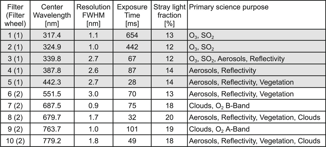
TABLE 1. Specifications of the EPIC filters. Filter wheel 1 with filters 1–5 is closer to the primary mirror, filter wheel 2 with filters 6 to 10 is closer to the detector. The center wavelengths are given in nm-air and the resolutions are given as the full width half maximum (FWHM) of the filter function. The exposure time is the one used in regular operation and is never changed. For the meaning of the stray light fraction see Stray Light Correction. The primary science purpose indicates for which science L2 product the respective channel is used.
This paper gives an overview of the mathematics and the pre-launch and on-orbit calibration behind the first of the steps above that is the basis for all further processes. Instrument Overview gives a short overview of the instrument design and performance. The different calibration periods are listed in Calibration Periods. L1a Processing Steps goes through each of the steps to convert the L0 data in L1a data. Pixel Size on Ground and Uncertainty discuss the EPIC pixel size on the ground and L1a data uncertainty, respectively. Conclusions are given in Conclusions.
Instrument Overview
The EPIC instrument is described in detail in the DSCOVR Overview report (Atmospheric Science Data Center, 2016; also https://epic.gsfc.nasa.gov/about/epic). Here we will provide a brief overview of the optical elements that are relevant for this paper. The optical path of EPIC is shown in Figure 1.
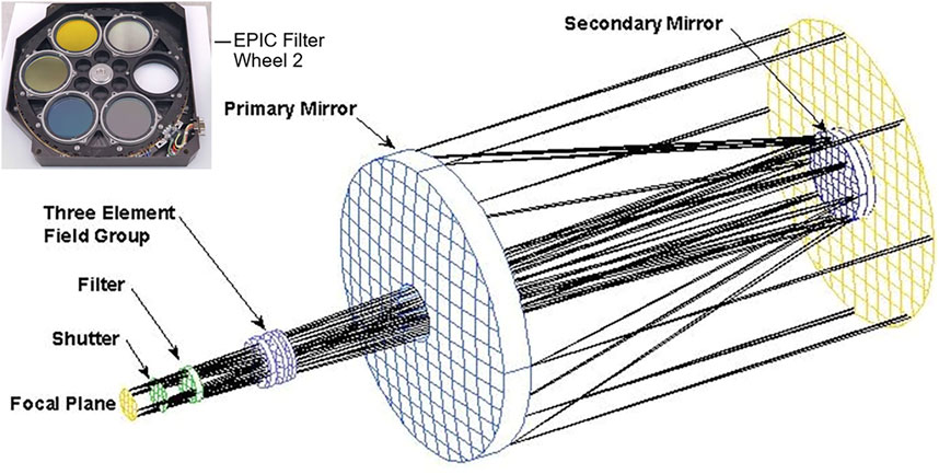
FIGURE 1. EPIC light path. The picture at the top left shows one of the filter wheels with six positions.
As light enters the front end of the 286 cm focal length Cassegrain telescope, it is reflected by the 30.5 cm diameter primary mirror onto the 9.5 cm diameter secondary mirror. Light reflected by the secondary mirror passes through the center of the primary mirror, where it enters the camera assembly. A three-element fused silica field lens group is designed to correct the inherent optical aberrations of the Cassegrain telescope such as coma, astigmatism, and field curvature. EPIC houses two filter wheels, each with six openings of 4 cm diameter, of which five are equipped with an optical filter and one position is left open (Figure 1). Each filter is a combination of a narrow band interference filter with a broadband blocking filter. The next element in the EPIC camera assembly is a 3-slit rotating shutter wheel to control the length of the exposure, i.e., the duration in which the detector actively collects photons of light. The filter specifications and the mission invariant exposure times for each channel used in orbit are given in Table 1.
In the focal plane of the beam is the EPIC detector, a thinned, backside-illuminated hafnium coated silicon wafer CCD with an anti-reflection coating. It contains 2,048 × 2,048 square pixels of 15 microns pitch, resulting in a total imaging area of slightly more than 3 × 3 cm2. In angular measurements, the pixel instantaneous field of view (iFOV) is 1.078 arcsecs. Therefore, the total field of regard (FOR) of the EPIC telescope is 0.607°, limited by the horizontal and vertical edges of the CCD (see Figure 2, where the gray areas in the corners of each panel show the region outside the FOV).
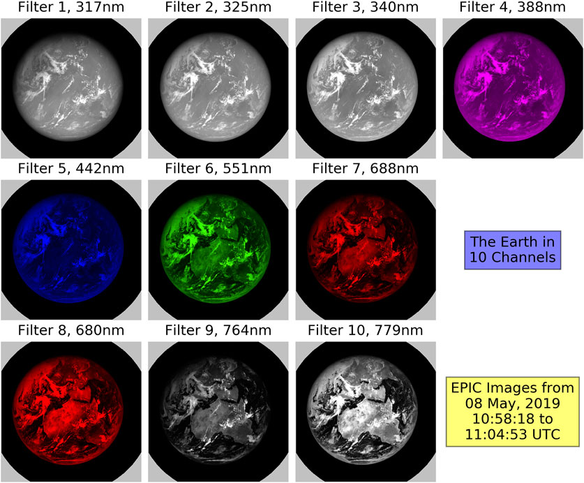
FIGURE 2. EPIC L1a images for each channel taken on May 8, 2019 around 11 UTC. One such full set of 10 images is taken by EPIC approximately every 65 min during the Northern Hemisphere summer and every 110 min during the Northern Hemisphere winter. The gray areas in the corners of each panel show the regions outside of the FOV of the telescope. Areas with no signal are plotted in black color. Higher signal intensity is plotted in shades of white for the UV filters 1 to 3 and the NIR filters 9 and 10 and for the visible filters in that color our eye would see if we placed the respective filter in front of it. The contrast between dark and bright areas in the images is smallest for the UV channels due to strong Rayleigh scattering, and increases with wavelength. The filter pairs 7–8 and 9–10 are relatively close in wavelength, but one channel in each pair is strongly absorbed by molecular oxygen (filters 7 and 9), which causes a much darker image of the Earth compared to the other filter in the pair.
The EPIC CCD can be drained (readout) from two opposite corners. In regular operation, the same corner is always used. If the readout through that corner fails, EPIC could switch to the readout from the other corner. While the entire EPIC calibration has been done for both readout modes, all results shown in this paper refer to the regular readout mode.
EPIC is read in a so-called “over-scanned” mode. This means although there are 2,048 × 2,048 pixels, 2,056 readings in both row and column direction are done. Therefore, the pixels from the first eight rows and columns do not include those photons that have been accumulated during the exposure time, but instead, only the photons caused by thermal electrons during the readout process. The pixels in these rows and columns are called “oversampled pixels” and are used in the dark correction (Dark Correction).
Calibration Periods
Most of the information used for the EPIC raw data calibration was obtained during calibration periods that are listed in this section. The first version of full calibration for EPIC L1a processing was finished before the launch of DSCOVR. The necessary measurements were obtained during two dedicated pre-launch calibration campaigns (Calibration Period “CalLM” and Calibration Period “CalGSFC”). This first calibration version was then modified based on information obtained during two on-orbit calibration campaigns (Calibration Period “CalDark” and Calibration Period “CalMoon”). Finally, the operational EPIC images are used to determine if the instrumental characteristics are changing with time. The observed small changes have been used to modify the calibrations.
Calibration Period “CalLM”
The first calibration period “CalLM” took place at the Lockheed Martin Advanced Technology Center, Palo Alto, CA. Preparatory measurements were taken in air and with the detector at room temperature during July and August 2011. Final measurements were obtained at flight conditions in the vacuum chamber with a cooled detector from 15–20 Sept 2011. More than 3,000 images were taken in total. The calibration setup for CalLM is described in detail by Cede et al. (2011). The light from a 1500W xenon lamp entered the vacuum chamber through a window into an integrating sphere. After exiting the sphere, the light passed a focusing lens and a selected “target” on the 6-position aperture wheel (most targets were holes of different diameters). Then it entered a Dobsonian collimator, which produced an extended beam with a divergence determined by the target. The beam was then reflected by the steering mirror and entered EPIC. This setup allowed EPIC to be illuminated with beams of different divergence, from point sources used for stray light calibration to extended sources that overfilled the instrument’s total FOV.
Calibration Period “CalGSFC”
The second pre-launch calibration period “CalGSFC” took place in February 2014 at NASA/Goddard Space Flight Center, Greenbelt, MD. In this period, measurements were taken in the vacuum chamber at flight conditions for 7 days with over 600 images in total. The focus was to repeat the original calibration sequences that did not give conclusive results in the 2011 tests during CalLM, namely the non-linearity and flat field calibration. In this calibration EPIC was illuminated by a beam reflected from a diffuser plate that overfilled the instrument’s FOV.
Calibration Period “CalDark”
The period from DSCOVR’s launch on February 11, 2015 to reaching its orbital location at the Earth-Sun Lagrange-1 point on June 7, 2015 was used for extensive dark count measurements with the closed telescope door and closed shutter and is called “CalDark”. More than 1,000 dark images were taken to complement the pre-launch dark count calibration.
Calibration Period “CalMoon”
At the beginning of the mission, EPIC was pointed towards the fully illuminated Moon instead of the Earth on several occasions in between regular operations (“lunar observations”). They were usually taken at times where the angular distance between Earth and Moon as seen from EPIC was at a maximum, which corresponds approximately to half-moon phases on Earth. The longest of these periods is called “CalMoon” and lasted from August 15–19, 2015, where the lunar surface was “moved” over 36 positions across the detector. Images for 5 filters were taken at each position. Additional shorter periods with lunar observations have been and continue to be inserted in the regular EPIC observations schedule (26 of such periods as of March 2021). The objectives of the lunar observations are to test the stray light and flat field calibrations, and to check the radiometric stability of EPIC over time.
L1a Processing Steps
Any measurement device has imperfections, so does EPIC. For example, the radiometric sensitivity and the dark counts vary across the detector, stray light affects the pixels in different ways, the readout mechanism has a latency, etc. In processing the raw L0 data to L1a data we try to correct for all such imperfections in the best possible way. This is done in several processing steps.
If everything was done “perfectly”, then each of the more than four million EPIC pixels would give exactly the same L1a output, if it was receiving the same input, and consequently the entire image only would need to be multiplied by one single number to convert from corrected count rates to radiances. Apart from the L1a data array, the L1a output also includes a so-called “pixel type array” of the same dimension as the image itself. The pixel types give information about whether the specific pixel is outside the EPIC FOV, is oversampled, is on or off “target” (i.e., inside or outside the disk of the Earth or the Moon), or is saturated or enhanced (see Enhanced Pixel Detection).
Some of the L1a corrections have less impact on the data than others. For those, the data would only differ from the “correct” data by a small amount if the correction was not applied. In order to get an overview of the magnitude (or impact) of each correction step, we decided to introduce “impact levels”, which allow a quick qualitative assessment of the impact each correction has on the data. Here we define four impact levels: “small” (impact is below 0.4%), “moderate” (between 0.4 and 2%), “significant” (between 2 and 10%), and “large” (above 10%). Note that these percentage limits have been chosen, since the magnitudes of the different corrections clustered approximately into groups limited by these numbers. Corrections may have a moderate impact on the image as a whole, but a significant impact on a subgroup of pixels that are especially affected by the respective effect. The nine processing steps are listed below, with the impact given in parenthesis. If two impact levels are given (e.g., significant to large), then the first one is for the average impact and the second one for the impact on the subgroup of more affected pixels:
• Step 1-Dark correction (moderate to large)
• Step 2-Enhanced pixel detection (small to large)
• Step 3-Read wave correction (small)
• Step 4-Latency correction (moderate to significant)
• Step 5-Non-linearity correction (small)
• Step 6-Temperature correction (small)
• Step 7-Conversion to count rates (small)
• Step 8-Flat fielding (significant to large)
• Step 9-stray light correction (significant to large)
In this section, we describe each correction step separately. Since it would go beyond the limits of this paper to describe each correction step in full detail, we focus on those corrections with more significant effects on the data, i.e., dark-count, flat-field, and stray light corrections.
Dark Correction
The first correction applied on the 12-bit digital resolution EPIC raw data is the dark correction. A rather “safe” way to perform dark correction on the data would be to add a dark measurement (i.e., a measurement with closed shutter) after every single regular measurement using the same exposure time (Table 1). In this way, the dark count would be measured with exactly the same conditions (e.g., electronic state and temperature of the detector) and, therefore, any possible systematic errors in the dark correction could be avoided. However, the download rate for DSCOVR is limited so that such a technique cannot be applied. Due to this limit, the operational EPIC images for all filters, except the 443 nm blue filter number 5, are reduced on the spacecraft from the original size of 2,048 × 2,048 pixels to 1,024 × 1,024 pixels by averaging each group of 2 × 2 pixels. This was the only way to keep the EPIC image sequence in the range of one set of 10 images every 65 min in the Northern Hemisphere summer and 110 min in winter. The difference is caused by the number of hours a single S-band receiving antenna located at Wallops Island, Virginia, United States is in view. As a consequence, the strategy for the dark correction was the following:
• Develop a model that determines the EPIC dark count at pixel i, DCi, based on two input variables, exposure time, tEXP, and detector temperature, TCCD, which are both transmitted in the auxiliary data.
• Adjust the modeled dark count to the electronic conditions at the measurement time using the oversampled pixels.
• Check the dark count behavior over time taking a daily dark measurement at 1,000 ms exposure time.
From the analysis of the data from CalLM, CalGSFC, and CalDark we developed the dark count model for dark count DCi at the ith pixel given in Eq. 1.
TREF is the reference temperature. It was originally set to −40.0°C, since this was the temperature the EPIC detector was expected to have in operation. After the CalDark period it was changed to −20.8°C, since this temperature was then effectively observed in the first months on orbit (Figure 3).
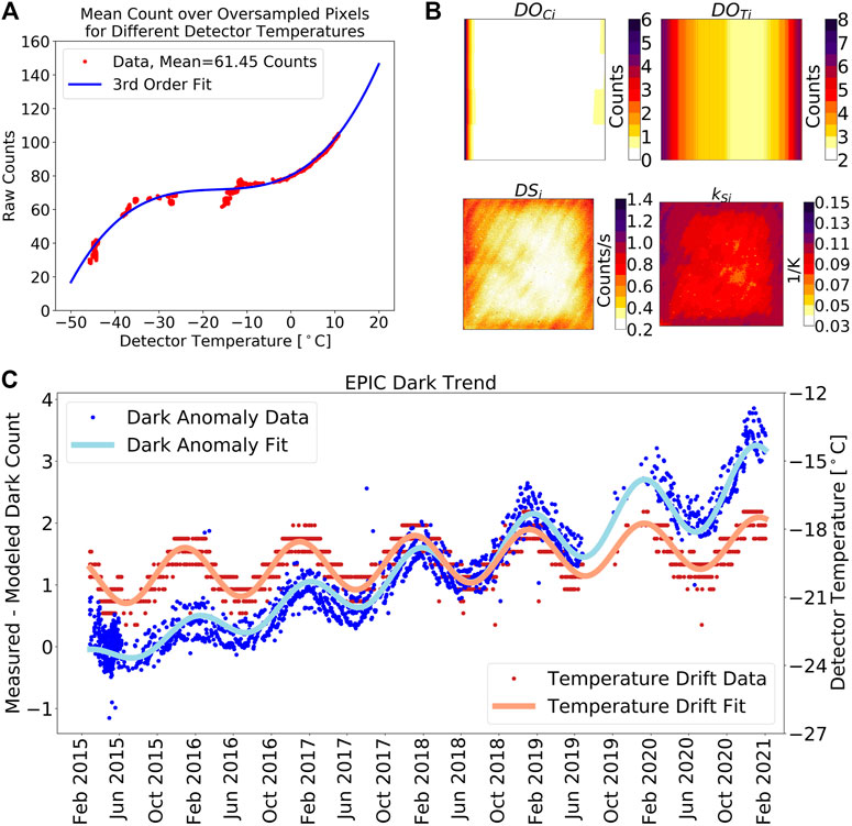
FIGURE 3. (A) DO0 as a function of TCCD measured during CalLM. (B) Dark model parameters DOCi, DOTi, DSi and kSi from Eq. 1. (C) EPIC dark trend. The apparent noise in the dark anomalies (blue dots) is mostly caused by the low resolution of 0.6 K for the detector temperature readings (red dots). Both data sets are fitted with formula y = a0+ a1· t + ( a3+ a5· t ) · sin[ 2 · π. ( t - a2)/a4], where t is the time in days since January 1, 2017 0:00 UTC. The obtained fitting parameters for the Dark Anomaly Fit (blue line) are : a0 = 0.71 counts, a1 = 0.49 counts/year, a2 = 71 days, a3 = 0.30 counts, a4 = 359 days, a5 = 0.07 counts/year. For the Temperature Drift Fit (red line): a0 = −19.69°C, a1 = 0.28 K/y, a2 = 94 days, a3 = 1.13 K, a4 = 368 days, a5 = −0.02 K/y.
The DO-terms represent the dark offset and are independent of tEXP. The dark slope DS depends linearly on tEXP. tIM is the time since January 1, 2017 0:00 UTC.
DOOV is the average dark count over the oversampled pixels (Figure 3). It is mostly a function of TCCD, but also depends on the electronic state of the detector system at the measurement time. This term does not need to be taken from the calibration, since it can be calculated for each operational measurement.
All 2,048 × 2,048 arrays DOCi, DOTi, DSi, and kSi from Eq. 1 are shown in Figure 3. DOCi gives the difference between the dark offset at each pixel and the value DOOV at standard conditions. As seen in Figure 3, DOCi increases towards the left edge of the detector, probably due to a temperature increase in this direction, and also shows a separation into four regions covering a quarter of the CCD each, which we believe is due to some characteristic of the readout electronics. The temperature dependence of the dark offset uses calibration parameters DOTi and kO. DOTi is mostly a function of the CCD columns (Figure 3) with kO determined to be 0.166/K.
The dark slope DS uses calibration parameters DSi and kSi. DSi is characterized by an increase at the readout corners due to elevated temperature and also shows a rather small number of hot pixels. Using as a criterion for a hot pixel to exceed the expected value by more than 10 counts at the reference temperature, then EPIC has 210 hot pixels, which is 0.005% of the total pixels. Since they are singular isolated pixels, they are not visible in Figure 3.
In the first calibration versions, the “trend term” DOT in Eq. 1 was not included in the dark model. It was added in 2017 when we discovered some pattern of the true dark count drifting away from the dark model as shown in Figure 3. This effect is clearly temperature-related but is obviously not correctly captured by the TCCD-dependent terms in Eq. 1, although they have been determined over a wide range of temperatures as seen in Figure 3. It turned out that adjusting the dark model with a modified TCCD-dependence was not possible, since the relation between the temperature and the observed dark count bias does not “fit” in the dark model framework. The seasonal temperature cycle of ±1.1 K is rather constant over time, while the seasonal cycle in the dark count bias changes from ±0.16 counts in 2015 to >±0.5 counts in 2020. Furthermore, the seasonal temperature cycle relates to the seasonal dark anomaly cycle on average by ∼0.3 counts/K, while the upwards trend in the temperature of ∼0.3 K/year causes an upwards trend of the dark count bias of ∼0.5 counts/year, i.e., a much higher relation of ∼1.7 counts/°C. Due to this discrepancy, we decided to define DOT as a function of the image acquisition time tIM with seasonal variation and a linear drift as shown in Figure 3. With this addition the dark model again well represents the true EPIC dark counts over its time in orbit.
Enhanced Pixel Detection
This L1a processing step only affects the pixel type array and does not change the L1a data array itself. The raw EPIC data can be saturated or enhanced. The invariant EPIC exposure times (Table 1) were selected on the first day of operation so that saturation rarely occurs, but it can still happen when a pixel views a highly reflective ice cloud high up in the atmosphere.
Enhanced pixels are pixels with physically impossible values that exceed the values of the neighbor pixels by a too large amount. This can be understood when looking at Figure 8, which shows the EPIC point spread function (more in Stray Light Correction). For example, based on this function it is not possible that the value in a pixel is five times larger than the average value over the adjacent pixels. We believe this enhancement is mostly caused by issues in the readout electronics. Nearly all EPIC images show a small percentage of enhanced pixels. Their number varies between just a few such pixels up to around 1,000 of them in a single image of four million pixels. An algorithm to detect enhanced pixels was developed. It is based on a comparison of the value in a pixel relative to the average value over its eight neighbor pixels. It then marks enhanced pixels in the pixel type array so that they can be ignored for science data products.
Read-Wave Correction
EPIC’s read-out electronics add a small sinusoidal wave to the image, called the “Read-wave”. This wave is a function of the image column and has a rather constant period between 10 and 11 pixels but varies from image to image in amplitude (between 0 and 0.6 counts) and phase. Both amplitude and phase are approximately constant for all rows. An example of such a read wave is shown in Figure 4. We developed an algorithm to determine the amplitude and phase of the wave for each measurement. It is based on fitting a sinusoidal wave into those rows of the image, which get no direct light input, i.e., the ones below and above the Earth’s disk, and then subtracting this wave from the entire image.
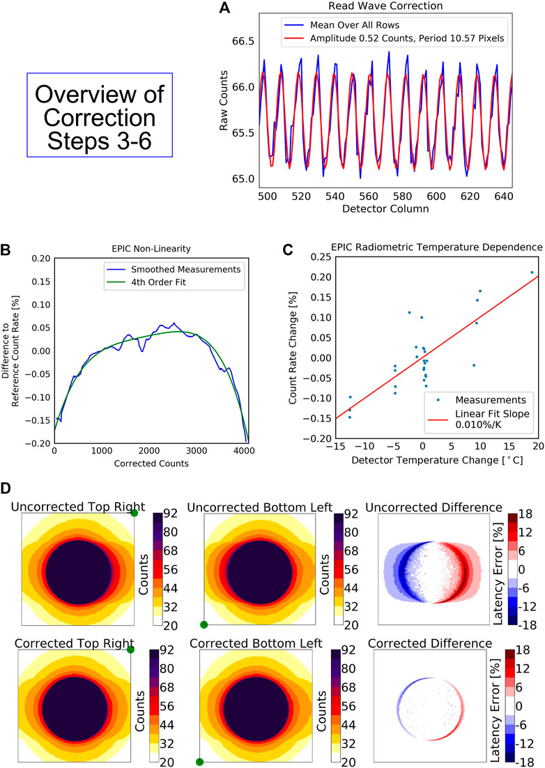
FIGURE 4. (A) Example for read wave for a dark count measurement. The blue line shows the average of the counts over all CCD rows between columns 495 and 645. The red line is a fitted sinusoidal wave, which is subtracted from the image for the read wave correction. (B) Measured (blue) and fitted (green) non-linearity of EPIC based on laboratory measurements during CalGSFC. (C) Measured and linearly fitted radiometric temperature sensitivity of EPIC based on laboratory measurements during CalGSFC. (D) Illustration of EPIC latency effect using measurements from CalLM. The exactly identical illumination, a circular illumination with a radius of 560 pixels, has been measured with two readout modes. One drains the image at the top right corner (see green dots), the other at the bottom left corner. The latency effect adds a positive bias to the data read just after the target, i.e., at the right side of the detector in the top left panel and at the left side in the top center panel. The top right panel shows the percentage difference of the panels (Top Right Corner minus Bottom Left Corner) before applying the latency correction. The bottom panels show the same images after the latency correction has been applied.
Latency Correction
Just like many imaging devices with a CCD, EPIC suffers from a so-called “latency effect”. That is, pixels with a low signal level are significantly biased high when they are read after a large number of pixels with a high signal level. This can cause an overestimation of as much as 12% in the signal from a low signal clear scene on Earth that is adjacent to a high signal extended region of clouds that is read just before it. The consequences of this bias have been analyzed for other satellite instruments (Várnai and Marshak, 2009).
The EPIC detector has two readout amplifiers located at opposite corners of the array, which allowed us to characterize the latency effect and develop a correction method for it. The method determines the additional charge Δi, which is accumulated in the readout electronics and added to the “true” signal Ci, which is the proper charge originating from the measured photons. We assume Δi = 0 for the first pixel i = 1 to be read, and for each subsequent pixel i+1, Δi+1 is given by Eq. 2:
kG and kD are the latent charge gain and decay constants, respectively, and have been determined to kG = 8.6 × 10⁻⁶ and kD = 3.7 × 10⁻³ for the regular readout mode based on measurements during CalLM. The effect is illustrated in Figure 4. Use of Eq. 2 reduces latency errors by a factor of 3.
Non-Linearity Correction
EPIC readout electronics underestimate very small (<500 counts) and very high signal levels (>3,500 counts) by up to 0.2% (Figure 4). This is a relatively small non-linearity effect and was characterized during CalGSFC.
Temperature Correction
EPIC shows a small radiometric temperature sensitivity of 0.01%/K (Figure 4), which is corrected in this step by using the onboard reading of the detector temperature. It was calibrated during CalGSFC, where images from a constant light source were taken over a temperature range from −40 to −10°C.
Conversion to Count Rates
The exposure time of an EPIC image is controlled by the shutter, which is a rotating disk with three open sectors of different angular width that moves in and out of the light path to unblock the incoming beam (Atmospheric Science DataCenter, 2016). The shutter is slightly non-linear, meaning that different pixels are exposed to light for a different amount of time. However, this shutter effect is only significant when the smallest sector (exposure times <10 ms) is used. For this reason, the filter bandwidths were decreased during refurbishment of EPIC to increase the exposure time to more than 20 ms so as to never use the smallest slit (Table 1). In this conversion step the data are divided by the invariant exposure time given in Table 1 to convert from “corrected counts” to “corrected count rates” (counts/s).
Flat Fielding
When EPIC is illuminated by a uniform input (i.e., each pixel receives exactly the same signal), the recorded image lacks uniformity for several possible reasons:
• Pixel response non-uniformity (PRNU): this is caused by small variations in the sensitivity of each pixel. It is independent of wavelength, has a very small spatial extent (i.e., changes from pixel to pixel), and a magnitude in the order of a few percent.
• Etaloning (ETAL): this is caused by optical interference effects from thickness variations in the depletion region of the CCD. It only affects longer wavelengths above 600 nm (hence only for EPIC filters 7–10), has a wider spatial extent than PRNU, and a magnitude of tens of percent.
• Surface inhomogeneity (INHOMO): this is caused by inhomogeneities on the detector surface, especially from the hafnium coating. It manifests as a localized reduction or enhancement of the sensitivity for a group of pixels with a magnitude of tens of percent. It has the same distribution, but different magnitudes for different channels, usually a stronger effect in the UV than in the visible, since hafnium is nearly transparent in the visible and NIR. Therefore, it manifests most in filters 1–4. The affected regions can have very different spatial extensions. Some features affect only a few pixels, while others spread over hundreds of pixels.
• Vignetting (VIGN): this is the reduction of the instrument sensitivity towards the periphery of the field of view. VIGN varies smoothly across the CCD and might be different for different filters. Based on optical modeling EPIC should not have strong VIGN, at most in the order of a few percent. It affects all EPIC channels in the same way, but it is best seen in filters 5 and 6, since the other filters are dominated by either ETAL (filters 7–10) or INHOMO (filters 1 to 4) as those effects have a much larger magnitude.
Due to the combination of the above described effects, the sensitivity of each EPIC pixel is different and a homogenous (or flat) illumination produces not at all a homogenous (or flat) image. Once the sensitivity across the detector, called the “flat-field response”, is known, the image can be divided by it, which is called “flat-field correction”. In the remainder of this section we describe how the EPIC flat-field response was determined.
In both pre-launch calibration campaigns CalLM and CalGSFC we attempted to produce an illumination as uniform as possible across the CCD. In CalLM the beam reaching EPIC was the output of a Dobson collimator telescope. In CalGSFC, EPIC was looking onto a large diffuser plate that was illuminated by a high-power tungsten halogen lamp. However, both inputs were far from being “flat” and showed gradients up to 30%. This forced us to accept some compromises for the pre-launch flat-field calibration.
We split the PRNU from the other effects described above, since it does not really need a flat input as long as the signal varies smoothly across the detector. It can be derived by comparing the value at a single pixel to the average value of the surrounding pixels. The final PRNU array is shown in Figure 5. It is applied separately from the other flat-field effects in the L1a data correction. We do not expect the PRNU to change over the mission lifetime.
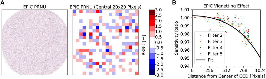
FIGURE 5. (A) EPIC Pixel response non uniformity as determined during CalGSFC. 61% of the pixels inside the telescopes’s FOV have an absolute value of the PRNU below 0.5%, 30% between 0.5 and 1.0%, 8% between 1.0 and 1.5%, 1% between 1.5 and 2.0 and 0.1% above 2.0%. (B) EPIC VIGN effect estimated from lunar observations during CalMoon. Each dot is the result of a single lunar image for the respective filter. The black line is a polynomial fit in all the data.
Instead of getting the absolute numbers for ETAL, INHOMO, and VIGN, we derived the combined result from these three effects relative to the 552 nm green filter 6, for which no flat field correction other than the PRNU was assumed or needed. The reason we picked filter 6 is that it is not affected by ETAL and we also observed very little INHOMO, as described in the next paragraph. In this way, it was possible to cancel out that part of the inhomogeneity of the input beam, which affects all filters in the same way.
The actual flat field maps are shown in Figure 6. We can observe that filters 1 to 4 are dominated by INHOMO, seen as regional depressions or enhancements across the detector. Filters 5 and 6 show much less INHOMO, with filter 6 even less than filter 5, which is the reason it was selected as the reference filter. Hence, they are dominated by VIGN. Finally, filters 7 to 10 are dominated by ETAL, seen as a pronounced variation over the entire detector. Overall, the flat-field correction for EPIC is on the order of ±25%. The magnitude of INHOMO was significantly different between CalLM and CalGSFC. We believe this is partly caused by the uncertainty in the laboratory measurements itself, but also originates from changes on the detector surface over pre-launch time from 2011–2014. We used the results from CalGSFC for the final pre-launch flat field correction, as they were closer to the launch date (2015). Due to these difficulties in the flat field calibration and the resulting large uncertainty, the plan was to re-evaluate and possibly modify the flat-field correction using in-flight data.
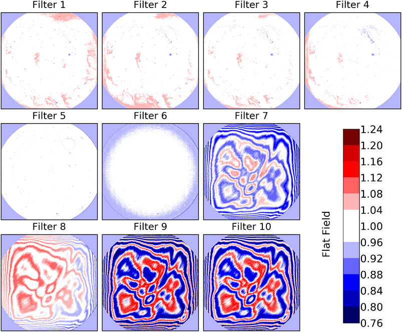
FIGURE 6. EPIC flat field maps without PRNU from the actual calibration version 18. Filters one to four are dominated by INHOMO, filters 5 and 6 by VIGN, and filters 7 to 10 by ETAL. The flat field correction consists of dividing the data in each filter by the arrays shown in this figure.
A first in-orbit modification of the flat-field calibration was performed in Fall 2016 using the fact that the telescope rotates about its optical axis with a six-months period. The idea was that when we average all the images of one filter over a long period, we should obtain a rather smooth image, since all features caused by the atmosphere and the ground should average out as they are “moving” across the detector. We saw that this assumption holds for small features, i.e., the resulting averaged image is rather smooth, but there are still systematic effects that cause an inhomogeneous result. For example, ocean glint, which creates an enhancement at the specular reflection angle near the center of the Earth (Várnai et al., 2020), and also the high albedo regions of Greenland and Antarctica, which cause higher backscattered signal away from the center of the image as they are at high latitudes. Therefore, we again fixed the flat field in filter 6 and only looked at the differences from it with this technique. The in-flight version of the flat field correction differed on average from the 1st version by <0.03% for filters 1–5, and in the range of 0.3–0.5% for filters 7, 9, and 10. However, in all filters there were extreme values, where the flat field changed for certain pixels by 34–53% in filters 1–5, and 9–15% for filters 7, 9, and 10. The technique did not seem to improve the flat field for filter 8 and therefore that channel was left unchanged. As a result of this improvement, L2 data such as the total ozone columns gave smoother and more consistent results (see Figure 7, left and middle panel).
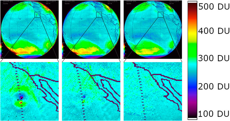
FIGURE 7. EPIC total ozone columns in Dobson Units (DU) on October 17, 2015 at 20:14 UTC using flat field calibration from pre-launch (left panels), the update from Fall 2016 (middle panels) and the actual latest version (right panels). The bottom row is a zoom into the region indicated by the black lines. The very low ozone values below 200 DU in a region of the bottom left panel are not real, as we know from other data, and are a consequence of the imperfect initial flat field correction. This artifact is not seen in the bottom right panel anymore, where the latest flat field correction is used.
The next improvement was to compare EPIC measured radiances for filters 1–4 with synthesized radiance images based on the NASA Ozone Mapping and Profiler Suite (OMPS) satellite (National Oceanic and Atmospheric Administration, 2021), while EPIC blue channel 5 was compared with the Ozone Monitoring Instrument (OMI) (Goddard Space Flight Center, 2021). For every EPIC radiance image, OMPS Nadir Mapper (NM) radiance spectra measured on the same day was convoluted with EPIC bandpass function and interpolated to the given EPIC channel wavelength. Then, the OMPS radiance measurements at EPIC wavelength were interpolated to each EPIC pixel geographic location. All of the nearly 6,000 synthesized images and as well as EPIC measured images from the first 18 months of the EPIC mission were averaged, respectively. Ratios of the averaged EPIC radiance image to the averaged OMPS radiance image were computed. The synthesized radiance images were corrected by accounting for the differences in the solar incidence angles and the satellite observation angles using the TOMRAD atmospheric radiative transfer model (Bhartia and Wellemeyer, 2002) and OMPS NM ozone retrieval results (ozone and surface reflectivity, etc.), which were also averaged and synthesized in parallel with the synthesizing of radiance images. Ratios of the averaged EPIC radiance image to the resulting OMPS (and OMI) radiance image were computed. This technique eliminates some large geophysical features mentioned above and characterizes pixel-to-pixel variations very well. However, we found the resulting flatfield still had significant offsets changing from the CCD-center to the edge. We believe this is because the spherical geometry approximation in TOMRAD causes increased uncertainties at large solar/viewing zenith angles. Also, the forward model does not simulate the ocean Sun glint. These two errors are circularly symmetric. Therefore, a polar coordinate system was set at the CCD center, and circles of CCD pixels were selected from the ratios and fitted with piecewise linear functions of the polar angle to determine a reference background. Pixels with large deviations from a fitted background were removed from the circle, and the raw ratios of the remaining pixels in the circle were fitted again. Two iterations of this fitting were performed. This procedure was repeatedly applied with 1-pixel radius increments from the center to the edge, where a sufficient (3,000) number of EPIC images were accumulated. Finally, the raw ratios were normalized with the resulting reference background for the flat field correction.
A further step to improve the flat-field correction was to estimate the magnitude of VIGN from the lunar measurements during CalMoon. After correcting for the slightly changing distances for Sun-Moon-EPIC, a given face of the Moon can be considered a stable light source. The obtained results for the EPIC sensitivity decrease towards the edge of the FOV and are shown in Figure 5. Since the scatter in the results was significantly larger than potential differences among the filters, we used a polynomial fit to the average over all filters as the final function for VIGN. The lunar calibration measurements are periodically repeated over the life of the mission.
The in-flight modifications described above further improved the quality of the L2 data like total ozone columns (Figure 7, right panel). The modification is on the order of up to 4% of radiance to optical speckle-like features in broad regions, and up to 60% for some bad pixels, which lead to corrections in the retrieved ozone from tens DU to hundreds DU. The estimated uncertainty in the flat field correction (pixel-to-pixel sensitivity changes) is 0.5%.
Stray Light Correction
Light entering EPIC from a specific direction does not only end up at the CCD location defined by geometric optics, the “core region” that consists of the corresponding pixel and its neighbor pixels. A fraction of the light is distributed over the entire detector as stray light. The fraction of the total signal ending up outside the core region, the “stray light fraction”, is rather large for EPIC, between 12 and 20% depending on the filter (Table 1). If not corrected, the stray light would severely reduce the quality of the scientific data products, particularly those depending on the ratio of light from different wavelength channels. Therefore, a stray light correction method based on the knowledge of the instrument’s point spread function (PSF) was developed. The method follows the principle described in Zong et al. (2006) used for a different purpose. To our knowledge this is the first time that such a technique has been applied to a 2-dimensional detector. Our novel approach is described in this section.
As mentioned in Calibration Periods, different targets were used during CalLM to create different illuminations for EPIC. For example, one target produced the circular image seen in Figure 4. Another target produced a quasi-parallel beam with divergence of ±5 × 10⁻⁵ degrees, which is only one third of the angular extension of one pixel, 3 × 10⁻⁴ degrees. When this “sub-pixel-illumination” was positioned to reach the CCD right in the center of a pixel, the obtained signal is considered to be the PSF of EPIC (Figure 8). Within the measurement uncertainty, the shape of the PSF for EPIC in the core region was found independent of the filter and the position on the detector.
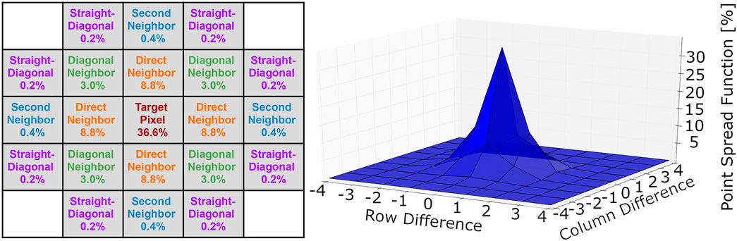
FIGURE 8. EPIC PSF in the core region measured during CalLM for filter 6 using sub-pixel-illumination. The data are normalized to the sum of the signal over the entire detector. The individual values are listed in the left panel. For filter 6, 87% of the signal ends up in the core region, i.e., the center pixel and the next neighbor pixels (cells with gray background), while 13% of the signal is stray light and spreads over the remaining part of the CCD. For other filters the shape of the PSF in the core region is the same, but the normalized values are different due to a different stray light fraction (Table 1).
When using the sub-pixel illumination, the signal outside the core region basically disappears in the measurement noise, i.e., the exact structure of the stray light cannot be determined. It was also not possible to increase the exposure time and saturate the center pixel to such an extent that this structure was seen. To solve this problem another target was used, which produces a beam with divergence of ±3 × 10⁻³ degrees or 3,600 times more energy than the sub-pixel illumination. This results in a “small circular image” with a radius of 20 pixels. Both unsaturated and saturated measurements with this target were taken and then merged to produce final images (Figures 9, 10). As in Figure 8, the data are normalized to the sum of the corrected signal over the entire detector. Several common features can be seen in the figures, but not all of them are related to stray light. For example, we believe that the enhancement of entire rows in the saturated regions is due to a not fully removed readout latency effect.
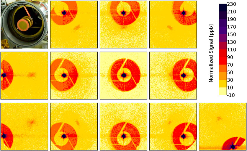
FIGURE 9. EPIC PSF in parts per billion (ppb) measured during CalLM for filter 8 using the small circular illumination directed at different positions on the detector. The top left panel shows the entrance of EPIC with the support structure of the secondary mirror.
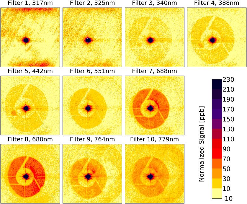
FIGURE 10. EPIC PSF measured during CalLM using the small circular illumination directed at the center of the detector for all filters.
The most obvious feature of EPIC stray light is a ghost image, in which the support structure of the secondary mirror can be seen. Based on optical modeling, we think this ghost image is mainly caused by reflections between the detector and the parallel filters, which are significant, although all of these optical elements have proper anti-reflection coatings applied. Since filter wheel 1 is farther away from the detector, the diameter of the ghost image is larger for filters 1 to 5 than for filters 6 to 10 (Figure 10).
Based on these measurements we developed a PSF-model for EPIC. For this model the PSF was divided into eight different “regions”: the core region with the 21 pixels shown in Figure 8, the near field, transition and interpolation regions, extending to a distance of ∼200 pixels around the center pixel (violet and dark red colors in the figures), the ghost image region (mostly orange colors in Figure 9), the regions inside and outside of the ghost (mostly yellow) and the region outside the telescope (the gray corners of Figure 2). The PSF-model consists of a set of filter-dependent parameters for each region, e.g., the stray light level in the transition region or the diameter of the ghost image region, etc. Details such as the arms of the support structure of the secondary mirror were omitted in the model (see also Figure 11). The PSF-model allows us to calculate an estimation of the EPIC PSF for each of the 10 filters for any of the more than four million pixels on the CCD.
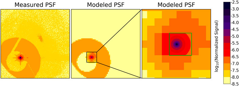
FIGURE 11. Measured (left panel) and modeled partially binned PSF (middle and right panels) for filter 8 at target pixel (1400,600) in logarithmic scale. The right panel is a zoom into the middle panel for the region of rows 1,250–1,550 and columns 450−750. The area inside the green frame in the right panel is the central part of 96x96 pixels around the target pixel, which is resolved in full resolution. Outside the green frame are the 32x32 “super-pixels”.
The next step in the stray light correction method described by Zong et al. (2006) is to build the so-called stray light distribution matrix D, which is basically the combination of all the PSFs. One column of D is the PSF with the core region replaced by zeros for the respective pixel as a column vector, i.e., with dimension (2,048 * 2,048 = 4194304,1) instead of (2,048, 2,048). The unitary matrix I is added to D. The result, I + D, is a diagonally dominant matrix with ones in the main diagonal and very small numbers elsewhere (values as shown in Figures 9, 10). I + D is inverted to obtain the stray light correction matrix C (Eq. 3).
D* is an approximation for the combined D-terms in Eq. 3 as is described below. C is then applied to the measured data (as a column vector) to correct for the stray light. The problem we faced is that for a 2D-detector like EPIC matrices D and C have a huge dimension (4194304, 4194304). Such a matrix would occupy >70 TB of disk space (for each filter) if stored in single precision. While it is in theory possible to create D using our PSF-model, it is completely impractical to invert D even with the most advanced computer system. And even if we were able to perform this inversion, applying matrix C to an image would also take far too much time to be executed for routine operation. Therefore, we made two simplifications:
First, we applied “partial binning” on the PSFs. The central part of 96 × 96 pixels around the target pixel is saved in full resolution, but all the pixels outside this central part are binned into “super-pixels” with a size of 32 × 32 pixels each. An example for this binned PSF is shown in Figure 11. The specific numbers for the configuration of the central part and the binning were a compromise between reducing the size of matrix C as much as possible and still maintaining a good measure of the stray light correction. This compromise was obtained by testing different configurations. The lower physical limit for the central part was about 90 × 90 pixels, since this covers the near field of the PSF (Figure 10), which has the strongest gradient. Any smaller size for the central region would have altered the results significantly. Since the width of the super-pixels must be an integer fraction of the pixel number in one dimension, 2,048, and the width of the central region must be a multiple of the width of the super-pixels (both for numerical reasons), the minimum possible size for the central region was then given by 96 × 96, as 96 is three times 32 or six times 16. Since we did not see a large difference between 32 × 32 and 16 × 16 super-pixels, we chose 32 × 32 as it significantly reduces the size of matrix C.
With these settings, the partially binned PSF has a total of 13,303 entries (9,216 pixels in the central part and in addition 4,087 super-pixels), which means the final stray light correction matrix C occupies ∼208 GB of disk space per filter in single precision. Despite this simplification, the operational stray light correction would still take a long time (roughly 52 min per image) when executed on a desktop computer. Instead, the operational EPIC data processing is done on a supercomputer at the NASA Center for Climate Simulation (NCCS) (National Aeronautics and Space Administration, 2021), where the processing can be done in less than 30 s per image.
The second simplification is that we approximate the inversion in Eq. 3 with only the first term of a Taylor series expansion, which can directly be obtained from the PSF-model. In order to compensate for the underestimation caused by the approximation I − D, we created a modified distribution matrix D* (Eq. 3). D* was obtained by testing the stray light correction on pre-launch and post-launch data with a known signal input.
Examples of such test images are shown in Figure 12. For the left panel in this figure, another target used during CalLM, the “bar target”, is measured. This target consists of rectangular areas with gaps in between. Knowing that the signal outside and in between the openings must be zero, we could fine-tune our PSF-model. These images were especially useful to test the performance of the stray light correction in the regions near the central pixel (the near field, transition, and interpolation regions), which is something that cannot really be verified after launch.
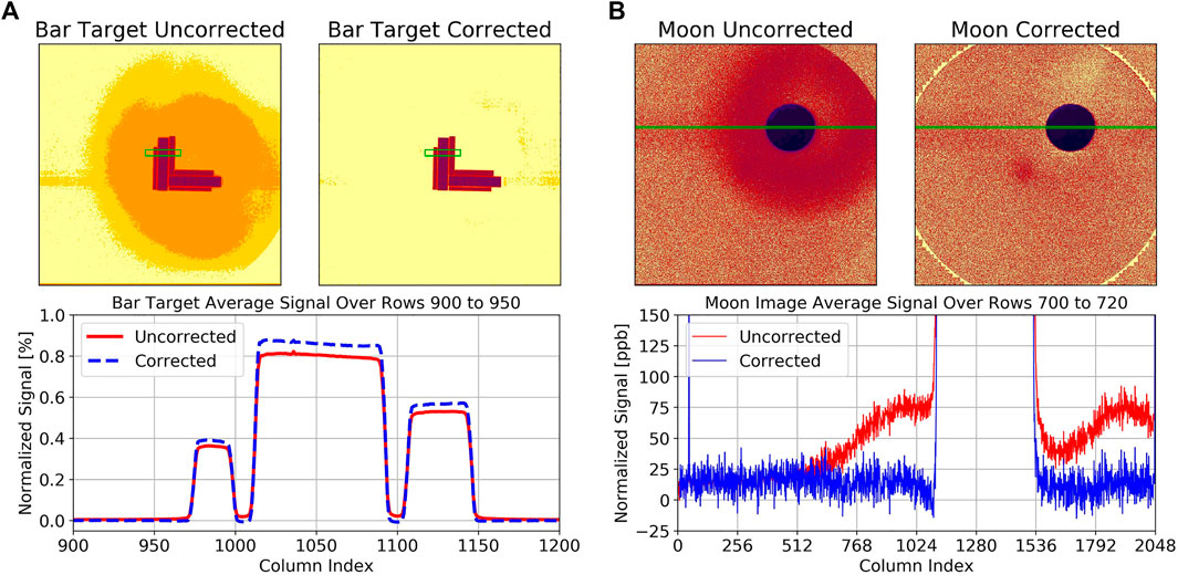
FIGURE 12. (All pseudo-color images are in logarithmic scales and use the same color bar as in Figure 11): (A) Bar target measurement for filter 8 from CalLM before stray light correction (“Uncorrected”) and after stray light correction (“Corrected”). The bottom panel shows the average over rows 900–950 as a function of the column index, which is indicated by the green area in the full images. The stray light reduces the signal at the maxima and fills the gaps in between the maxima (red solid line). After the correction (dashed blue line) the signal at the maxima is “restored” and the signal in the gaps caused by the stray light is “cleared”. (B) Lunar image for filter 8 from CalMoon before stray light correction and after stray light correction. The bottom panel shows the average over rows 700–720 as a function of the column index, which is indicated by the green line in the images. Before the correction (red line) the signal outside the lunar surface is enhanced, mostly due to the ghost image, while after the correction (dashed blue line) it is approximately zero.
The right panel in Figure 12 shows a lunar image taken during CalMoon. While we could not use the region on the moon itself to test the stray light correction, since we do not know the exact structure of the lunar surface, we could make use of the fact that outside the moon the signal must be basically zero and that the signal drops sharply to zero at the edge of the lunar disk since the moon has no atmosphere.
One check for the quality of the stray light correction that can be done for the operational data is simply to look at the region outside the target (Earth or Moon), which should give a signal as close to zero as possible. We have analyzed the ratio R of the mean signal outside the Earth <SOUT> over the mean signal on the Earth <SON> for the first year of EPIC data in orbit, R = <SOUT>/<SON>. For eight of the filters, R ranged from 0.8–2.7% before stray light correction was applied, and from −0.1%–+0.4% after the correction, which proves excellent performance of the stray light correction algorithm of a factor of 7 or higher. An exception is filter 9, where the numbers are 3.5 and 1.0%, respectively, hence, still an improvement by a factor 3.5, but not of the same quality as for the other filters.
Another way to test the quality of the stray light correction is described in Geogdzhaev and Marshak (2018), where absolute calibration constants for EPIC filters 5, 6, 8, and 10 are found through comparison with data from the Moderate Resolution Imaging Spectroradiometers (MODIS) onboard the Terra and Aqua satellites. The authors applied their technique separately for dark scenes and bright scenes. When EPIC L1a calibration, especially the stray light correction, was done correctly, the two methods should give approximately the same calibration constants. Their analysis showed that the agreement between the calibration based on the dark and bright scenes respectively increased by a factor of 1.7–3.3 after EPIC stray light correction was applied.
Figure 13 shows the stray light error (SLE) for the same images as shown in Figure 2, i.e., from May 8, 2019 around 11:00 UTC. Here we define the SLE as the percent difference between the data before and after the stray light correction. The median of the SLE-distribution for the pixels on the Earth’s disk (“pixels on Earth”) ranges from −2% for filters 1 to 5 down to −4% for filter 8. This is because stray light causes a fraction of the energy from the pixels on Earth to spread to the pixels outside the Earth’s disk (“pixels outside Earth”). For the pixels outside Earth, the SLE goes towards infinity since the corrected data are close to zero. Bright scenes (clouds, ice or high surface albedo like over Africa for the higher filters) have a negative SLE, which ranges from −6% for filters 1–6 down to −10% for filter 8 (this is based on the 1-percentile of the SLE-distribution for pixels on Earth). Dark scenes (clear sky and low surface albedo) have a positive SLE, which can exceed the scale of Figure 13 substantially with values above 50% and even up to 100% for filter 8 (this is based on the 99-percentile of the SLE-distribution for pixels on Earth).
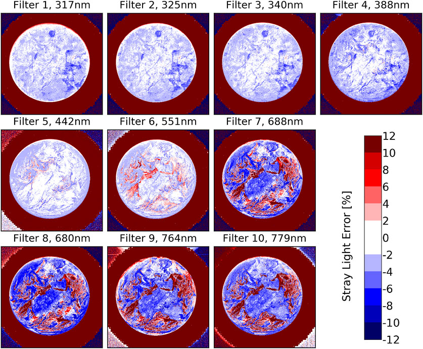
FIGURE 13. Stray light error for the EPIC images from Figure 2 (May 8, 2019 around 11:00 UTC).
Pixel Size on Ground
An important question for the data user is where does the light come from as measured by one EPIC pixel? This is often referred to as the “footprint” of a satellite pixel. The answer to this question is strongly related to the PSF, which describes how the light originating from a point source is distributed over the CCD. The core part of the EPIC PSF (Figure 8) can be approximated by a 2-dimensional super Gaussian function with exponent 1.63 ± 0.11 and FWHM of 1.29 ± 0.11 pixels. The angular FOV of a pixel is given by the core PSF “mirrored on the center point” and convoluted over the extension of the pixel. It describes the angles where light originates that ends up on a given pixel. The FWHM of the EPIC FOV, which is obviously a 2D super-Gaussian just like the PSF, is 1.73 arcsecs. The geographic footprint finally is the projection of the angular FOV on the Earth’s surface, i.e., one needs to include the distances, angles, etc., included in the telemetry. The blue lines in Figure 14 show the footprint for the “standard case” of normal incidence on the ground (satellite viewing zenith angle VZA = 0°) and the average Earth-Lagrange 1 distance. For this situation, the footprint is approximately circular with a FWHM of 12.5 km, a 50% energy contour line with a diameter of 13.2 km (i.e., 50% of the energy measured in the pixel is from within this circle) and a 90% energy contour line with diameter of 24.9 km. The footprint increases with the distance of EPIC from the Earth and also changes in size and shape for other places on the Earth with VZA > 0°.
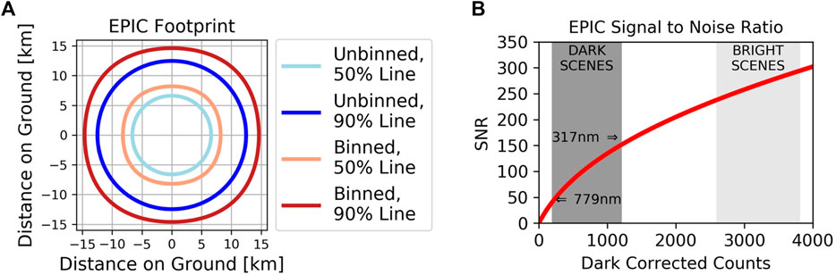
FIGURE 14. (A) Energy contours of the EPIC footprint for a pixel at 0° satellite zenith angle and average Earth-Lagrange 1 distance. The blue lines represent the unbinned case, the red lines the case of 2 × 2 binned pixels. The light colors give the 50% level, i.e., 50% of the energy reaching the pixel comes from inside this region. The dark colors give the 90% level. (B) EPIC SNR for the operational readout mode at typical CCD temperatures. The SNR of dark scenes is smaller in the visible than in the UV due to the larger contrast between dark and bright scenes (see also Figure 2).
As already mentioned in Dark Correction, the images from all filters except the blue filter 5 are “binned”, i.e., the averages over groups of 2 × 2 pixels are formed. The FOV for one of these binned pixels increases to 2.41 arcsecs, since the convolution is done over a larger area than in the unbinned case. This also changes the native footprint of the L1a data for these filters (red lines in Figure 14). The “binned” footprint is not circular anymore and has a FWHM of 17.5 km, a 50% energy contour line with a diameter of 16.4 km and a 90% energy contour line with diameter of 29.2 km.
Uncertainty
A complete uncertainty analysis for EPIC L1a data has not been made, since this is outside of the available resources. However, we can determine the read noise and the gain of EPIC, which allows us to estimate the signal to noise ratio (SNR) of an EPIC measurement:
CC are the dark corrected counts ranging from 0 to about 4,000. CC can be approximated by multiplying the L1a data (count rates) with the exposure times given in Table 1. NREAD is the read noise, which is 3.9 counts for the operational EPIC readout mode. GAIN = 0.04 on average (it changes with the CCD temperature). The SNR is shown in Figure 14. It ranges from 50:1–150:1 for dark scenes (lower values for higher wavelengths and higher values for short wavelengths that have significant Rayleigh scattering) and from 250:1 to 300:1 for bright scenes containing clouds or snow/ice. A measure of the success of the corrections is that features as small as 10 km can be discerned (Nile river banks) in the 443 nm blue channel and that the very sensitive algorithm for ozone retrieval is successful (Kramarova et al., 2021 submitted).
For the binned images (all filters but filter 5), the SNR is the double of the numbers shown in Figure 14 and listed in the previous paragraph for L1a data.
Conclusion
We believe that within the available possibilities from pre-launch and on-orbit calibration activities, an adequate EPIC raw data calibration has been obtained. The produced L1a data are corrected for all known instrumental effects and only need to be multiplied by a single number for each filter to obtain absolute calibrated radiances from the count rate. Before in-flight data were available, it was decided that no attempt would be made to determine the conversion from count rates to radiances for two reasons. First, the laboratory setup to produce an absolutely calibrated, homogenous, extended light source is a rather difficult task and would have exceeded the possibilities with respect to budget and schedule. Second, it is unlikely that the absolute calibration values obtained during pre-launch would have been applicable to the operation on orbit, as many factors, such as launch stress or the different environment and instrument illumination in space, usually modify the calibration significantly (see, e.g., Kabir et al., (2020). Therefore, the EPIC L1a data are given as corrected count rates and the 10 numbers needed to convert to radiances are determined by comparison to other satellites in a later processing step.
Several of the corrections described in L1a Processing Steps follow well-established procedures for instrument calibration. However, for some of the steps, we needed to develop rather novel techniques that have not been previously used to our knowledge.
• A readout latency correction method was determined. This was possible since the EPIC detector can be drained (read) from different CCD corners and the necessary measurements were made before launch (Latency Correction).
• The flat-field corrections, which turned out to be the most critical part with respect to producing reliable L1a data, needed to be adjusted on-orbit relative to their pre-launch values. This was done through comparison with other satellites and by applying a statistical analysis of all the EPIC images taken over a long period (Flat Fielding).
• A novel stray light correction method was developed based on partially binned PSFs to handle the huge dimensions of the matrices involved (Stray Light Correction).
Since its launch in 2015, EPIC has been monitored for possible calibration changes, e.g., the dark count evolution (Dark Correction), the number of hot pixels (Enhanced Pixel Detection), or the radiometric stability from periodic lunar observations. The overall conclusion is that the observed instrumental changes are small, which we attribute to the benevolent conditions for the Lagrange 1 orbit. EPIC does not undergo periodic variations of extremely hot and cold temperatures like satellites in Earth orbits (low Earth orbits or geostationary orbits), which periodically move from sun to shadow, for low Earth orbits every ∼50 min. Furthermore, it is in a much more constant radiation environment compared to the instrument in LEOs, which cross the South Atlantic Anomaly (SAO) at least once per day [see, e.g., Li et al. (2020)]. Since the same side of the DSCOVR satellite always points to the Sun, the shielded effect from charged particles originating from the solar wind is much better than the charged particle effect in the SAO. We believe that apart from the excellent Earth-observing situation from Lagrange 1, the observations discussed in this document are another positive aspect of this orbit, which should be considered when possible future missions are discussed.
Data Availability Statement
The raw data supporting the conclusions of this article will be made available by the authors, without undue reservation.
Author Contributions
All authors have contributed to conception and design of the study and manuscript revision, and have read, and approved the submitted version.
Funding
The work was supported through different grants by the NASA DSCOVR program managed by R. S. Eckman, specifically grants NNX15AB57G, NNX15AN07G, NNX17AC97G, 80NSSC18K0992, and 80NSSC19K0769.
Conflict of Interest
AC is co-owner of SciGlob Instruments & Services LLC and LuftBlick. GM was employed by SciGlob Instruments & Services LLC. LH was employed by Science Systems and Applications, Inc.
The remaining authors declare that the research was conducted in the absence of any commercial or financial relationships that could be construed as a potential conflict of interest.
Acknowledgments
The authors and the DSCOVR project would like to thank the EPIC refurbishment and calibration efforts of the Lockheed-Martin team headed by Joseph Mobilia. Resources supporting this work were provided by the NASA High-End Computing (HEC) Program through the NASA Center for Climate Simulation (NCCS) at Goddard Space Flight Center.
References
Atmospheric Science DataCenter (2016). Deep Space Climate Observatory, Earth Science Instrument Overview. Report available under (Accessed February 18, 2021).
Bhartia, P., and Wellemeyer, C. (2002). “TOMS-V8 Total O3 Algorithm,” in OMI Algorithm Theoretical Basis Document, (Greenbelt, MD, USA: NASA Goddard Space Flight Center). Vol. II, 15–31.
Carn, S. A., Krotkov, N. A., Fisher, B. L., Li, C., and Prata, A. J. (2018). First Observations of Volcanic Eruption Clouds from the L1 Earth-Sun Lagrange Point by DSCOVR/EPIC. Geophys. Res. Lett. 45 (20), 11456–11464. doi:10.1029/2018GL079808
Cede, A., Mobilia, J., Demroff, H., Sawyer, K., Hertzberg, E., and Herman, J. (2011). Stray Light in EPIC. San Francisco, CA, USA: AGU Fall Meeting. December 5-9, 2011.
Christian, K., Wang, J., Ge, C., Peterson, D., Hyer, E., Yorks, J., et al. (2019). Radiative Forcing and Stratospheric Warming of Pyrocumulonimbus Smoke Aerosols: First Modeling Results with Multisensor (EPIC, CALIPSO, and CATS) Views from Space. Geophys. Res. Lett. 46, 10061–10071. doi:10.1029/2019GL082360
Davis, A. B., Ferlay, N., Libois, Q., Marshak, A., Yang, Y., and Min, Q. (2018). Cloud Information Content in EPIC/DSCOVR's Oxygen A- and B-Band Channels: A Physics-Based Approach. J. Quant. Spectrosc. Radiat. Transfer 220, 84–96. doi:10.1016/j.jqsrt.2018.09.006
Doelling, D., Haney, C., Bhatt, R., Scarino, B., and Gopalan, A. (2019). The Inter-calibration of the DSCOVR EPIC Imager with Aqua-MODIS and NPP-VIIRS. Remote Sens. 11, 1609. doi:10.3390/rs11131609
Geogdzhaev, I. V., and Marshak, A. (2018). Calibration of the DSCOVR EPIC Visible and NIR Channels Using MODIS Terra and Aqua Data and EPIC Lunar Observations. Atmos. Meas. Tech. 11, 359–368. doi:10.5194/amt-11-359-2018
Goddard Space Flight Center (2021). Aura | Ozone Monitoring Instrument. Available at: (Accessed March 31, 2021).
Herman, J., Huang, L., McPeters, R., Ziemke, J., Cede, A., and Blank, K. (2018). Synoptic Ozone, Cloud Reflectivity, and Erythemal Irradiance from Sunrise to sunset for the Whole Earth as Viewed by the DSCOVR Spacecraft from the Earth-Sun Lagrange 1 Orbit. Atmos. Meas. Tech. 11, 177–194. doi:10.5194/amt-11-177-2018
Herman, J., Cede, A., Huang, L., Ziemke, J., Torres, O., Krotkov, N., et al. (2020). Global Distribution and 14-year Changes in Erythemal Irradiance, UV Atmospheric Transmission, and Total Column Ozone For2005-2018 Estimated from OMI and EPIC Observations. Atmos. Chem. Phys. 20, 8351–8380. doi:10.5194/acp-20-8351-2020
Kabir, S., Leigh, L., and Helder, D. (2020). Vicarious Methodologies to Assess and Improve the Quality of the Optical Remote Sensing Images: A Critical Review. Remote Sens. 12, 4029. doi:10.3390/rs12244029
Kramarova, N., Ziemke, J., Huang, L. K., and Herman, J. (2021). Evaluation of Version 3 Total and Tropospheric Ozone Columns from EPIC on DSCOVR for Studying Regional Scale Ozone Variations. Front. Remote Sens. (submitted June 2021).
Li, C., Krotkov, N. A., Leonard, P. J. T., Carn, S., Joiner, J., Spurr, R. J. D., et al. (2020). Version 2 Ozone Monitoring Instrument SO2 Product (OMSO2 V2): New Anthropogenic SO2 Vertical Column Density Dataset. Atmos. Meas. Tech. 13 (11), 6175–6191. doi:10.5194/amt-13-6175-2020
Lyapustin, A., Go, S., Korkin, S., Wang, Y., Torres, O., Jethva, H., et al. (2021). Retrievals of Aerosol Optical Depth and Spectral Absorption from DSCOVR EPIC. Front. Remote Sens. 2. doi:10.3389/frsen.2021.645794
Marshak, A., and Knyazikhin, Y. (2017). The Spectral Invariant Approximation within Canopy Radiative Transfer to Support the Use of the EPIC/DSCOVR Oxygen B-Band for Monitoring Vegetation. J. Quant. Spectrosc. Radiat. Transfer 191, 7–12. doi:10.1016/j.jqsrt.2017.01.015
Marshak, A., Herman, J., Adam, S., Karin, B., Carn, S., Cede, A., et al. (2018). Earth Observations from DSCOVR/EPIC Instrument. Bull. Am. Meteorol. Soc. 99 (9), 1829–1850. doi:10.1175/BAMS-D-17-0223.1
Meyer, K., Yang, Y., and Platnick, S. (2016). Uncertainties in Cloud Phase and Optical Thickness Retrievals from the Earth Polychromatic Imaging Camera (EPIC). Atmos. Meas. Tech. 9, 1785–1797. doi:10.5194/amt-9-1785-2016
Molina García, V., Sasi, S., Efremenko, D. S., Doicu, A., and Loyola, D. (2018). Radiative Transfer Models for Retrieval of Cloud Parameters from EPIC/DSCOVR Measurements. J. Quant. Spectrosc. Radiat. Transf. 123, 228–240. doi:10.1016/j.jqsrt.2018.03.014
National AeronauticsSpace Administration (2021). NASA Center for Climate Simulation: High Performance Computing for Science. Available at: (Accessed March 18, 2021).
National OceanicAtmospheric Administration (2021). Joint Polar Satellite System: Ozone Mapping and Profiler Suite. Available at: (Accessed March 5, 2021).
Pisek, J., Arndt, S. K., Erb, A., Pendall, E., Schaaf, C., Wardlaw, T. I., et al. (2021). Exploring the Potential of DSCOVR EPIC Data to Retrieve Clumping Index in Australian Terrestrial Ecosystem Research Network Observing Sites. Front. Remote Sens. 2. doi:10.3389/frsen.2021.652436
Sasi, S., Natraj, V., Molina-Garcia, V., Efremenko, D. S., Loyola, D., and Doicu, A. (2020). Model Selection in Atmospheric Remote Sensing with an Application to Aerosol Retrieval from DSCOVR/EPIC, Part 1: Theory. Remote Sens. 12, 22. doi:10.3390/rs12223724
Song, W., Knyazikhin, Y., Wen, G., Marshak, A., Mõttus, M., Yan, G., et al. (2018). Implications of Whole-Disc DSCOVR EPIC Spectral Observations for Estimating Earth’s Spectral Reflectivity Based on Low-Earth-Orbiting and Geostationary Observations. Remote Sens. 10, 1594. doi:10.3390/rs10101594
Torres, O., Bhartia, P. K., Taha, G., Jethva, H., Das, S., Colarco, P., et al. (2020). Stratospheric Injection of Massive Smoke Plume from Canadian Boreal Fires in 2017 as Seen by DSCOVR-EPIC, CALIOP and OMPS-LP Observations. JGR Atmospheres 125 (10), e2020JD032579. doi:10.1029/2020JD032579
Várnai, T., and Marshak, A. (2009). MODIS Observations of Enhanced clear Sky Reflectance Near Clouds. Geophys. Res. Lett. 36 (6). doi:10.1029/2008gl037089
Várnai, T., Kostinski, A., and Marshak, A. (2020). Deep Space Observations of Sun Glints from marine Ice Clouds. IEEE Remote Sens. Lett. 17 (5), 735–739. doi:10.1109/LGRS.2019.2930866
Weber, M., Hao, D., Asrar, G. R., Zhou, Y., Li, X., and Chen, M. (2020). Exploring the Use of DSCOVR/EPIC Satellite Observations to Monitor Vegetation Phenology. Remote Sensing 12, 2384. doi:10.3390/rs12152384
Wen, G., Marshak, A., Song, W., Knyazikhin, Y., Mõttus, M., and Wu, D. (2019). A Relationship between Blue and Near-IR Global Spectral Reflectance and the Response of Global Average Reflectance to Change in Cloud Cover Observed from EPIC on DSCOVR. Earth Space Sci. 6, 1416–1429. doi:10.1029/2019EA000664
Xu, X., Wang, J., Wang, Y., Zeng, J., Torres, O., Reid, J., et al. (2019). Detecting Layer Height of Smoke Aerosols over Vegetated Land and Water Surfaces via Oxygen Absorption Bands: Hourly Results from EPIC/DSCOVR in Deep Space. Atmos. Meas. Tech. 12, 3269–3288. doi:10.5194/amt-12-3269-2019
Yang, K., and Liu, X. (2019). Ozone Profile Climatology for Remote Sensing Retrieval Algorithms. Atmos. Meas. Tech. 12, 4745–4778. doi:10.5194/amt-12-4745-2019
Yang, W., Marshak, A., Varnai, T., and Knyazikhin, Y. (2018). EPIC Spectral Observations of the Variability in Earth's Global Reflectance. Remote Sens 10 (2), 254. doi:10.3390/rs10020254
Yang, Y., Meyer, K., Wind, G., Zhou, Y., Marshak, A., Platnick, S., et al. (2019). Cloud Products from the Earth Polychromatic Imaging Camera (EPIC) Observations: Algorithm Description and Initial Evaluation. Atmos. Meas. Tech. 12, 2019–2031.[1]. doi:10.5194/amt-12-2019-2019
Yin, B., Min, Q., Morgan, E., Yang, Y., Marshak, A., and Davis, A. (2020). Cloud Top Pressure Retrieval with DSCOVR-EPIC Oxygen A and B Bands Observation. Atmos. Meas. Tech. 13, 1–18. doi:10.5194/amt-13-1-202010.5194/amt-13-5259-2020
Zhou, Y., Yang, Y., Gao, M., and Zhai, P-W. (2020). Cloud Detection over Snow and Ice with Oxygen A- and B-Band Observations from the Earth Polychromatic Imaging Camera (EPIC). Atmos. Meas. Tech. 13 (3), 1575–1591. doi:10.5194/amt-13-1575-2020
Keywords: Satellite remote sensing, Earth observation, Lagrange 1 point, instrument calibration, flat field correction, stray light correction
Citation: Cede A, Kang Huang L, McCauley G, Herman J, Blank K, Kowalewski M and Marshak A (2021) Raw EPIC Data Calibration. Front. Remote Sens. 2:702275. doi: 10.3389/frsen.2021.702275
Received: 29 April 2021; Accepted: 23 June 2021;
Published: 09 July 2021.
Edited by:
Yongxiang Hu, National Aeronautics and Space Administration, United StatesCopyright © 2021 Cede, Kang Huang, McCauley, Herman, Blank, Kowalewski and Marshak. This is an open-access article distributed under the terms of the Creative Commons Attribution License (CC BY). The use, distribution or reproduction in other forums is permitted, provided the original author(s) and the copyright owner(s) are credited and that the original publication in this journal is cited, in accordance with accepted academic practice. No use, distribution or reproduction is permitted which does not comply with these terms.
*Correspondence: Alexander Cede, YWxleGFuZGVyQHNjaWdsb2IuY29t