 Yaping Zhou
 Yuekui Yang1
 Peng-Wang Zhai
 Meng Gao
94% of researchers rate our articles as excellent or good
Learn more about the work of our research integrity team to safeguard the quality of each article we publish.
Find out more
ORIGINAL RESEARCH article
Front. Remote Sens., 15 July 2021
Sec. Atmospheric Remote Sensing
Volume 2 - 2021 | https://doi.org/10.3389/frsen.2021.690010
This article is part of the Research TopicDSCOVR EPIC/NISTAR: 5 years of Observing Earth from the first Lagrangian PointView all 24 articles
With the ability to observe the entire sunlit side of the Earth, EPIC data have become an important resource for studying cloud daily variability. Inaccurate cloud masking is a great source of uncertainty. One main region that is prone to error in cloud masking is the sunglint area over ocean surfaces. Cloud detection over these regions is challenging for the EPIC instrument because of its limited spectral channels. Clear sky ocean surface reflectance from visible channels over sunglint is much larger than that over the non-glint areas and can exceed reflectance from thin clouds. This paper presents an improved EPIC ocean cloud masking algorithm (Version 3). Over sunglint regions (glint angle ≤25°), the algorithm utilizes EPIC’s oxygen (O2) A-band ratio (764/780 nm) in addition to the 780 nm reflectance observations in masking tests. Outside the sunglint regions, a dynamic reflectance threshold for the Rayleigh corrected 780 nm reflectance is applied. The thresholds are derived as a function of glint angle. When compared with co-located data from the geosynchronous Earth orbit (GEO) and the low Earth orbit (LEO) observations, the consistency of the new ocean cloud mask algorithm has increased by 4∼10% and 4∼6% in the glint center and granule edges respectively. The false positive rate is reduced by 10∼17%. Overall global ocean cloud detection consistency increases by 2%. This algorithm, along with other improvements to the EPIC cloud masks, has been implemented in the EPIC cloud products Version 3. This algorithm will improve the cloud daily variability analysis by removing the artificial peak at local noon time in the glint center latitudes and reducing biases in the early morning and late afternoon cloud fraction over ocean surfaces.
When the geometric configuration of Sun, surface, and viewing angles form a mirroring path, the specular reflection, or sunglint, creates a bright spot on the remote sensing imagery. Ocean surface reflectance in the visible spectrum over sunglint is much larger than that from other areas. If the ocean surface were perfectly smooth, sunglint would appear in remote sensing images as the mirror image of the Sun, occupying a relatively small portion of the images. In reality, because of the wave and ocean currents, the ocean surface is tilting toward different directions, causing the sunlight to scatter and resulting in a large area of glint zone. The size of the glint zone in the satellite imagery depends on the ocean surface roughness, which in turn can be parameterized in terms of the vector wind field. The classical work by Cox and Munk (1954a), Cox and Munk (1954b) use sea surface wind speed and direction 10 m above the ocean surface to parameterize the distribution probability of the orientation of sea surface facets, which is widely used in radiative transfer models to estimate glint distribution and intensity.
The large reflectance in the glint region poses significant problems in the remote sensing of some atmospheric and ocean constituents. For example, remote sensing of atmospheric aerosol over ocean relies on separating the total sensor reflectance originated from surface and atmospheric molecular and aerosol backscattering. While surface reflectance over ocean can be estimated with auxiliary wind information, aerosol retrieval is normally avoided near and in the sunglint region (glint angle <40°) because of the large uncertainties (Levy et al., 2005). Likewise, sunglint is a serious confounding factor for remote sensing of water column properties and benthos as the total signal is dominated by the sunglint which makes the retrieval of water-leaving radiance very difficult (e.g., Khattak et al., 1991; Hagolle et al., 2004; Ottaviani et al., 2008; Kay et al., 2009; Jackson and Alpers, 2010; Harmel and Chami, 2013).
Outside the sunglint regions, cloud detection over ocean surfaces is considered relatively easy due to the sharp contrast between bright cloud objects and the generally dark ocean surface in the visible spectral channels. A single reflectance test at 0.86 µm can detect over 95% of daytime clouds over water when compared to the full set of Moderate Resolution Imaging Spectroradiometer (MODIS) cloud mask tests (Zhou et al., 2003). The MODIS cloud mask algorithm utilizes a varying reflectance threshold for the 0.86 µm channel in sunglint regions, where they are split into three sections according to the sunglint angle Θglint. For Θglint from 0 to 10°, the mid-point threshold is constant at 0.105, for Θglint from 10° to 20° the threshold varies linearly from 0.105 to 0.075, and for Θglint from 20° to 36°, it varies linearly from 0.075 to 0.055 (Frey et al., 2008; Ackerman et al., 2010). Additional spectral tests in thermal and near infrared channels are useful in delineating between clear sky and some optically thin clouds.
The Earth Polychromatic Imaging Camera (EPIC) on board the Deep Space Climate Observatory (DSCOVR) launched in 2015 has 10 narrow spectral channels in the ultraviolet (UV) and visible/near-infrared (Vis/NIR) (317–780 nm) spectral regions. The DSCOVR satellite, which is located in the first Lagrangian (L1) point of the Earth–Sun orbit, approximately 1.5 million kilometers away, allows the EPIC instrument to take continuous measurements of the entire sunlit side of the Earth from the nearly backscattering direction (scattering angles between 168.5 and 175.5∘) every 1∼2 h (Marshak et al., 2018; Yang et al., 2019). The geometric configuration of EPIC leads to a large sunglint zone close to the center of each 2024x2024 CCD pixel granule (e.g., Figure 1A).
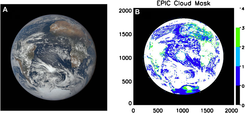
FIGURE 1. (A) Example of EPIC RGB image for the granule at 13:31 UTC on January 1, 2016. (B) Cloud mask for this granule from Version 2 (old) cloud mask algorithm. Notice the enhanced glint reflectance in the center of the granule in (A) and corresponding false positives of cloud identification in the glint region in (B). Blue, light blue, green, and white colors indicate four levels of cloud mask output: confident clear, uncertain clear, uncertain cloud and confident cloud, respectively.
A suit of cloud products, including cloud mask (CM), cloud effective pressure (CEP), cloud effective height (CEH), and cloud optical depth (COD), have been developed with observations from the EPIC’s 10 spectral channels (Yang et al., 2019). EPIC possesses two oxygen (O2) band pairs each with an absorption channel and a non-absorption reference channel. The A-band absorption channel is centered at 764 nm with a full width at half maximum (FWHM) of 1.02 nm, and its reference channel is centered at 780 nm with a FWHM of 1.8 nm. The B-band's absorption channel is centered at 688 nm with a FWHM of 0.84 nm, and its reference channel is centered at 680 nm with a FWHM of 1.6 nm (Marshak et al., 2018). Oxygen absorption has been applied to remote sensing of cloud and aerosol extensively (e.g., Fischer and Grassl, 1991; Stammes et al., 2008; Wang et al., 2008; Ferlay et al., 2010; Ding et al., 2016; Richardson et al., 2020). The EPIC’s two O2 band pairs (R764∕R780 and R688∕R680) are used for the retrieval of CEP (Yang et al., 2013; Davis et al., 2018a; Yang et al.,2019; Yin et al., 2020) and for cloud masking over snow and ice (Zhou et al., 2020). The retrieval is based on the principle that the O2 absorption bands are sensitive to the presence of clouds, especially high and thick clouds that reduce the absorbing air mass that light travels through while the reference channel does not. An increase in the ratio of the bidirectional reflectance functions (BRFs) between the absorbing and reference channel can not only indicate the presence of cloud but also be used to retrieve the effective cloud height (Yang et al., 2013; Yang et al., 2019). Zhou et al. (2020) further improved the O2 band ratio-based cloud mask algorithm over snow and ice by developing a dynamically varying threshold with surface altitude and Solar/view zenith angles.
Over ocean, the Version 2 (old) EPIC cloud mask algorithm uses the Rayleigh corrected reflectance of 680 and 780 nm channels with fixed thresholds (Yang et al., 2019). The Rayleigh correction partially mitigated the angle effect. EPIC cloudmask algorithm generates four levels of clear and cloud confidences similar to those of official MODIS cloud mask (Table 1). The global mean cloud fraction over ocean derived from EPIC is within 3% of those computed from collocated LEO/GEO composites. The pixel level accuracy of EPIC cloud mask product is about 88% (Yang et al., 2019). Though the performance is reasonable, further inspection reveals that over sunglint regions near the center of the granules, the algorithm nearly always identifies pixels as cloudy regardless of whether or not clouds are present (Figure 1). This increases the cloud fraction around local noon time over the ocean at latitudes where sunglint occurs. In addition, we also noticed that the cloud mask for ocean pixels near the edge of the granules is biased toward cloudy, which is due to enhanced reflectance in the large solar/view zenith angles near the edge. This bias can lead to an overestimation of cloud fraction close to the edge of the images, including high-latitude regions. It is worth noting that the biases in the cloud mask affect the EPIC downstream products as well. For example, the EPIC COD retrieval procedure (Meyer et al., 2016), which adopts a single channel retrieval approach similar to what Yang et al. (2008) describes, uses cloud mask as part of the input.
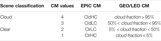
TABLE 1. Cloud mask classification from EPIC and GEO/LEO. CldHC, CldLC, ClrLC, ClrHC stand for cloud with high confidence, cloud with low confidence, clear with low confidence, and clear with low confidence, respectively.
This study aims to improve the EPIC cloud mask over the sunglint region and granule edges over ocean based on the radiative transfer simulations and collocated observations from GEO/LEO platforms. A new application of the A-band ratio in the glint region will be investigated. The remainder of the paper is organized as follows: First, we introduce the data and radiative transfer model (RTM) used and the sensitivity studies conducted. Then we will describe EPIC’s sunglint distribution and impact. Next we will describe the new ocean cloud mask algorithm including the threshold derivation and algorithm evaluation. Then we will discuss impact of the new algorithm on cloud diurnal cycle and zonal mean oceanic cloud fraction. Summary and discussion will be provided in the end.
The primary data used in the study are the EPIC level 1B calibrated reflectance and the EPIC level 2 standard cloud products (Yang et al., 2019). In addition, the study uses the composite cloud product developed by the Clouds and the Earth’s Radiant Energy System (CERES) team at the NASA Langley Research Center as reference for comparison with the EPIC cloud detection results. The composite is created by projecting the geosynchronous Earth orbit (GEO) and low Earth orbit (LEO) satellite retrievals to the EPIC grid at each EPIC observing time (Khlopenkov et al., 2017; Su et al., 2018). The procedure ensures that every EPIC image/pixel has a corresponding GEO/LEO composite image/pixel with approximately the same size and observing time. The LEO satellites include NASA Terra and Aqua MODIS and NOAA AVHRR, while geosynchronous satellite imagers include the Geostationary Operational Environmental Satellites (GOES) operated by NOAA, Meteosat satellites by EUMETSAT, and Multifunctional Transport Satellites (MTSAT) and Himawari-8 satellites operated by the Japan Meteorological Agency (JMA). The time differences between the GEO/LEO and the EPIC observations are included in the product files. To limit uncertainties, we only use pixels where the GEO/LEO and EPIC observations are within 5 min of each other. Compared to EPIC, the GEO/LEO sensors are usually better equipped for cloud detection because more spectral channels are available in these instruments. The cloud retrievals in the composite data follow Minnis et al. (2011). Because of EPIC’s large pixel size, one EPIC pixel corresponds to many GEO/LEO pixels each with its own cloud mask and optical properties retrievals; hence a composite pixel reports a cloud fraction based on cloud masks of the GEO/LEO pixels within it.
An EPIC simulator (Gao et al., 2019) has been developed based upon an RTM (Zhai et al., 2009; Zhai et al., 2010) that solves multiple scattering of monochromatic light in the atmosphere and surface systems. The model setup is described in Gao et al. (2019), Zhou et al. (2020). The EPIC simulator is used to generate the oxygen A-band and B-band reflectance over ocean surface. Gas absorptions due to ozone, oxygen, water vapor, nitrogen dioxide, methane, and carbon dioxide are incorporated in all EPIC bands. The gas absorption cross sections are computed from the HITRAN line database (Rothman et al., 2013) using the Atmospheric Radiative Transfer Simulator (ARTS) (Buehler et al., 2011). Line broadening caused by pressure and the temperature dependencies of line absorption parameters are considered. In the O2 A- and B-bands, radiances from line-by-line radiative transfer simulations are conducted and then convolved with the EPIC instrument response functions. The model atmosphere uses Standard US atmosphere profile from Intercomparison of Radiation Codes in Climate Models (ICRCCM) project (Barker et al., 2003) and assumes a one-layer cloud with a molecular layer both above and beneath. The O2 absorption within clouds is considered by assuming a fixed O2 molecule vertical profile.
The cloud is assumed to be liquid droplets following a gamma size distribution with an effective radius of 10 µm and an effective variance of 0.1. The cloud layer has varied optical thickness ranging from 0.2 to 30 and cloud top height (CTOP) from 1.0 to 15 km above the ground. The cloud geometrical thickness (CGT) varies from 0.5 to 4 km. The model simulates a variety of cases with 17 solar zenith angles (SZAs) ranging from 0 to 80∘, 18 view zenith angles (VZAs) from 0 to 85∘, and 37 relative azimuth angles (RAZMs) from 0 to 180∘, all with an increment of 5∘. The lower boundary is an ocean surface with the surface roughness characterized by the Cox Munk model (Cox and Munk, 1954a; Cox and Munk, 1954b). A fixed surface wind speed of 6 m/s is used (Gao et al., 2019). The model simulated reflectance under similar sun-view geometry to the EPIC observations are used for developing thresholds for cloud detection.
The sunglint region of an image can be roughly estimated by the glint angle (Θglint), which denotes the angle between the reflection received by satellite sensor and the angle of specular reflection. The glint angle is defined as
where θs, θv, and Φ are the solar zenith, the satellite zenith and the relative azimuth angles (between the Sun and the satellite), respectively. Glint contamination are normally considered within [0°, 30°] or [0°, 40°] depending on applications.
Figure 2 shows glint covered area from a single granule (Figure 2A), an entire day (Figure 2B) to an entire year (Figure 2C). Based on the sunglint contamination on cloud mask, we define our glint region in this study as a region with glint angle less than 30°. Figure 2 shows that sunglint covers a large fraction of a granule in the granule center if the region happens to be ocean. At any given day, the glint center moves from east to west and creates a zonal band of about 30° in the meridional direction where the glint is centered (Figure 2B). June 21 and December 21 represent the north (south) most position of the Sun (and glint center latitude) respectively. The glint center is located near the equator on March 21. Because sunglint appears in the entire oceanic part of the latitudinal band, if included, it is sufficiently large to affect the oceanic cloud fraction diurnal cycle analysis, and possibly mean cloud fraction in those latitudes due to the bias in the Version 2 cloud mask. This issue has been noticed by the community. For example, in the analysis of Delgado-Bonal et al. (2020), the time period with sun-glint is excluded. Lastly, the glint center migrates between 23°S–23°N each year and creates a total glint contamination region spanning from -38° to 38° (Figure 2C). Figure 2D shows the percentage of ocean area in each latitude which ranges from around 50% in 40°N to more than 95% in 40°S. The glint effect of the mean zonal cloud fraction is expected to be larger in southern hemisphere, with a larger percentage of ocean coverage.
FIGURE 2. (A) Glint angles for a single granule from September 24, 2017, 04 UTC. The thick red line in the middle is the location of the simulations shown in Figures 3, 4. (B) Glint areas (within 30° of glint angle) in all granules drawn from left to right as the day progresses on June 21, March 21, and December 21, 2016 in the top, middle and low rows, respectively; pink, light pink, and pale represent areas within 10, 20 and 30 degrees of glint angle. (C) Glint migration during a year. Red, pink, light pink and light purple colors mark the boundaries of 0° and 10°, 20°, 30° of glint angles. (D) Ocean area percentage at each latitude.
It is important to correct the cloud mask bias in the sunglint area. The simulation of Gao et al. (2019) shows that while clear sky ocean reflectance increases over sunglint regions, the presence of thin clouds dims the glint reflectance. While this makes single reflectance threshold tests difficult, they also find that the cloudy sky A-band ratio is usually higher than that of clear sky in the glint region, making it a potential test for cloud mask in the glint region. In the following section, we will further investigate the behavior of A-band ratio in the glint region and try to incorporate it in the ocean cloud mask algorithm.
To demonstrate the effect of sunglint on reflectance over the ocean, the reflectance at 780 nm R780 from the EPIC simulator along a horizontal line passing the center of one granule from September 24, 2017 (Figure 2A) is shown (Figure 3). Hypothetical ocean surface is assumed everywhere. The clear sky R780 is smaller than those of cloudy sky outside the sunglint zone, but increases toward the center and surpasses the cloudy sky R780 for thin clouds with optical thickness less 3. The cloudy sky R780 generally increases with cloud optical depth (COD), even at the glint center except when clouds are very thin (COD <1). The R780 of cloudy sky is always larger than that of clear sky outside the sunglint zone, and is insensitive to cloud height (figure now shown), which makes it a good candidate for cloud detection for ocean surface outside sunglint zone. Inside the sunglint zone, however, R780 for cloudy sky can be larger or smaller than that of clear sky depending on cloud optical thickness, hence a single R780 test cannot always separate clear and cloudy pixels.
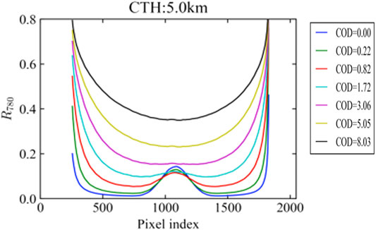
FIGURE 3. Model simulations of reflectance at 780 nm for clear sky and cloud with different optical thickness along the horizonal line passing the granule center in Figure 2A. Clear sky is in color blue.
The ratio of A-band behaves quite differently than the 780 nm channel. In the center of glint, A-band ratio of clear skies is always smaller than those of cloudy skies, regardless of cloud optical thickness and cloud height (Figure 4). The separation between clear sky and cloudy sky A-band ratio increases with cloud height and optical thickness. For low cloud at 2.5 km, a clear separation between cloudy sky and clear sky in A-band ratio would require a cloud optical thickness greater 2, while for clouds with height greater than 5 km, a thin cloud with optical thickness greater than 0.82 is sufficient to separate the two. This is due to the greater sensitivity of the absorbing channel to the cloud height and optical depth as discussed in Zhou et al. (2020). Exact conditions (combination of COD and height) of clouds that can be detected would depend on the measurement uncertainty, which is estimated to be around 1% after considering the cancelation of calibration errors in the two bands (Davis et al., 2018b). The clear sky A-band ratio in the glint center is around 0.38; hence a difference between cloudy sky and clear sky A-band ratio larger than 0.04 would be above the 1% uncertainty range. It is found that 82% of the pixels at the glint center (Θglint < 20°) with a cloud at 2.5 km and COD of 1.72 can satisfy this condition. Outside the sunglint region, the clear sky A-band ratio can be higher or lower than cloudy sky depending on the cloud height and COD. This renders the A-band ratio test only good for the sunglint region where the surface reflectance is high. To summarize, the EPIC R780 can serve as a good test for cloud detection outside the sunglint region; inside the sunglint, the EPIC O2 A-band ratio can be used to separate clear and cloudy pixels when R780 fails for thin clouds.
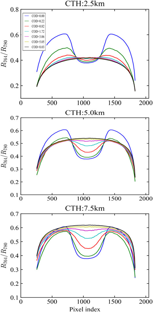
FIGURE 4. Model simulations of A-band ratio (R764/R780) for clear sky (blue curve, COD = 0) and cloudy sky with different cloud optical thickness (COD) (see color legend) and cloud top height (CTH) at (A) 2.5 km, (B) 5 km, and (C) 7.5 km along a horizonal line passing the granule center in Figure 2A.
To derive stable thresholds for the EPIC instrument, additional investigation is necessary to examine the clear and cloudy sky data under all possible EPIC Sun-view geometry. For this purpose, we selected one EPIC granule from each month in 2016 and extracted the Sun-view geometry for all the pixels in this dataset. This creates a representative dataset for the EPIC Sun-view geometries. The EPIC simulator results are then interpolated into all the Sun-view angles in this dataset. Figure 5 shows that the EPIC R780 and A-band ratio as a function of Θglint. The sawtooth appearance in the figure is due to the Sun-view angle spread and corresponding R780 for a given Θglint. As shown in the figure, there is a well-defined curve of R780 and A-band ratio as a function of Θglint from clear sky simulations for most of the ocean areas. The clear sky R780 increases at the glint center (Θglint < 30°) and spreads slightly that overlaps with thin clouds (COD <1.7) (Figure 5A). It remains quite flat, though not completely constant, at the Θglint range of 40°∼120° before rising sharply again at Θglint > 150° with an even larger spread. Importantly, the A-band ratio for clear skies is consistently lower than that of thin clouds in the glint region (Figure 5B). The curves show that it is possible to define tabulated baseline thresholds in 1° intervals for cloud detection by combining the R780 and A-band ratio tests.
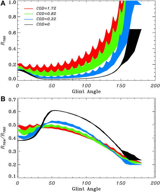
FIGURE 5. Ensembles of simulated (A) 780 nm reflectance and (B) A-band ratio with geometries from 12 EPIC granules (one per month) in 2016. Black, blue, green and red shows simulations from COD = 0.0, 0.22, 0.82, 1.72, respectively. Cloud top height is 5 km and geometric thickness is 3 km.
In this section we examine the observed Rayleigh corrected R780 (R′780) and A-band ratio as a function of Θglint (Figure 6). Choosing Rayleigh corrected reflectance is to minimize the known angle effect. The separation of clear sky and cloudy sky is based on the results derived from the collocated GEO/LEO cloud fraction (Su et al., 2018). The upper bounds of the model-simulated clear sky of R′780 and A-band ratio are plotted for comparison. We notice that the upper bounds of the model derived clear sky R′780 and A-band ratio (solid lines) represent the lower and upper bounds of their observed counterparts, respectively. The observed clear sky R′780 distribution shows a high concentration of low values in the middle range of the glint angles, but increases toward both ends, similar to what is shown in Figure 5. There is more spread (toward higher values) in the clear sky R′780 distribution than that of the simulation, possibly due to cloud contamination in the GEO/LEO dataset (also notice that the clear sky category we define for GEO/LEO may contain some cloud, see Table 1). The spread is larger with larger Θglint due to larger pixel size; hence more likely cloud contamination. The cloudy sky R780 is generally higher than those for the clear sky at the same Θglint except at very small Θglint (<25°), where a large portion of the clear sky and cloudy sky R′780 are in the same range. The model simulated R780 envelops the observed reflectance in both clear sky and cloudy sky plots outside the glint region, which makes it a good candidate as a cloud masking test. On the other hand, the model simulated clear sky A-band ratio curve falls between observed cloudy sky A-band ratios, indicating that it is not an ideal test beyond the glint region. As expected, the large spread of the observed clear sky A-band ratio narrows towards the glint center where most clear sky values are under the simulated curve. Inside the glint region, however, the cloudy sky A-band ratio is mostly higher than that of the clear sky, which indicates that the A-band ratio can be used as a test in the glint region.
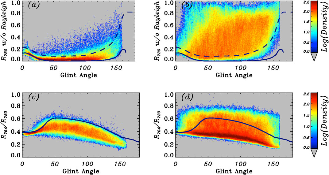
FIGURE 6. Observed Rayleigh corrected EPIC 780 nm reflectance (A,B) and A-band ratio (C,D) as a function of glint angles from January and July 2017 for clear sky (A,C) and cloudy sky (B,D). The solid black lines represent the upper bounds of the model simulated clear sky Rayleigh corrected R780 in each 1-degree glint angle bins. Dash lines represent the adjusted Rayleigh corrected R780 thresholds.
Based on these observations, we designed the cloud mask ocean algorithm as follows:
For Θglint < 25°,
R′780 > R0 => cloud
R′780 < R0 and R764/R780 > A0 => cloud
For Θglint > 25°,
R′780 > R0 => cloud
where the R0The improvement of the new algorithm can be easily examined visually, as more than 2/3 of the granules have sunglint in the ocean. Figure 7 shows the new cloud mask for the granule at 13:31 UTC on January 1, 2016 shown in Figure 1. The new cloud mask algorithm eliminates the obvious overestimate of clouds in the glint center while keeping small cloud features in the glint intact. It is also noticeable that the old cloud mask overestimates cloud coverage in most of the edge areas of the granule (Figure 2B), especially on the right side, and the new algorithm has mitigated this issue as well.
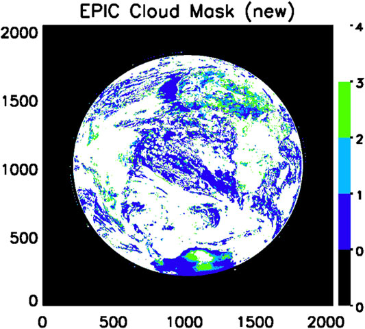
FIGURE 7. New cloud mask for the granule at 13:31 UTC on January 1, 2016 shown in Figure 1. The new algorithm shows mostly clear sky with small features of cloud consistent with the cloud pattern outside the sunglint region.
To quantitatively evaluate the new cloud mask, we conducted a comparison with the CM from the Langley LEO/GEO composite product introduced in Data and RTM simulations. As in Zhou et al. (2020), we divide the GEO/LEO cloud fraction into four categories to match with the four confidence levels of CM in EPIC (Table 1).
In addition, we define the accuracy, probability of correct detection rate (POCD) and probability of false detection rate (POFD) as:
where a is the number of pixels that both algorithms identify as cloudy (including high and low confidence), b is the number of pixels that both identify as clear (including high and low confidence), c is the number of pixels that EPIC identifies as clear while GEO/LEO identifies as cloudy, and d is the number of pixels that EPIC identifies as cloudy while GEO/LEO identifies as clear. We note that the cloud detection in GEO/LEO is by no means the truth, hence the “accuracy” here should be interpreted as consistency with GEO/LEO rather than true accuracy. The same should be applied to POCD and POFD as they are relevant to GEO/LEO’s cloud detection.
Figure 8 shows the matchups between EPIC cloud mask in 1 (blue), 2 (cyan), 3 (yellow), 4 (red) with the GEO/LEO cloud fraction with <5%, 5–50%, 50–95% and >95% categories. It is obvious that the old algorithm overestimates the cloud in the glint center, evidenced by a red bar in the first group where GEO/LEO has low cloud fraction (<5%) and virtually no blue bar in high cloud fractions (>95%) categories. The new algorithm increases the blue bar (high confident clear sky) in the clear region without overestimating clear sky in the cloudy region. Similarly in the high Θglint region (toward granule edge), the new algorithm was able to detect more clear sky (blue bar) in the clear region without overestimating clear sky in the cloudy region. Improvement is evident for the new algorithm, where most of the pixels with <5% cloud fraction have CM = 1 or 2 (high and low confidence clear, respectively), while pixels with >95% cloud fraction more likely have CM values of four and 3 (high and low confidence cloudy, respectively). In the glint center, the overall consistency increases from 81.9 to 86.9% and POFD decreases from 17.3 to 7.3%. In the large glint angle region, the consistency increases from 80.3 to 86.6% and POFD decreases from 20.7 to 9.5%. For the entire global ocean, the improvement in the glint center and granule edge leads to an improvement of consistency from 86.6 to 88.7% and false detection rate from 10.2 to 6.7%. The improvements in other months are similar to that of January and July 2017 (Table 2). Based on these results, the new ocean cloud mask algorithm increases the detection consistency in the glint center and granule edges by 4∼10% and 4∼6%, respectively, with a reduction of false cloud detection rate by 10∼17%. Overall global ocean cloud detection consistency increases by approximately 2%.
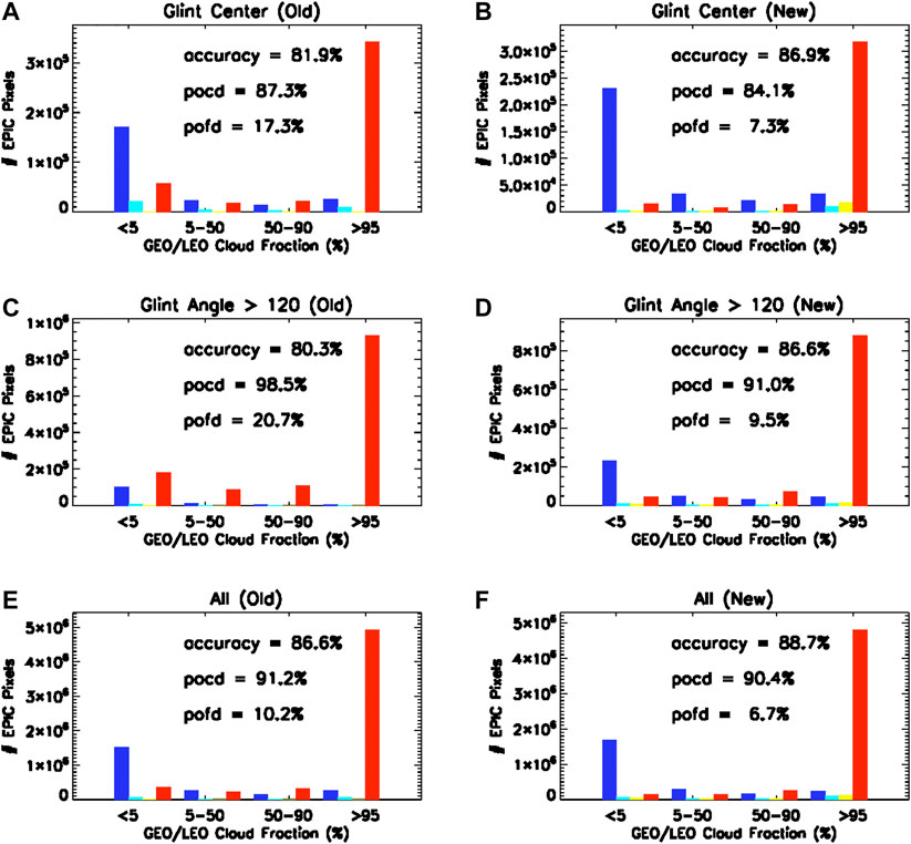
FIGURE 8. Number of pixels in each pixel-by-pixel matchup category between the cloud mask from EPIC and cloud fraction from GEO/LEO composite over ocean surfaces for January and July 2017 at glint center (Θglint < 25°) (A,B); large glint angles (Θglint > 120°) (C,D), and all glint angles (E,F). Left is from Version 2 EPIC cloud mask algorithm and the right is from the new algorithm. Blue, cyan, yellow, and red bars are for EPIC cloud mask equals to 1, 2, 3, 4, respectively. POCD: probability of correct detection; POFD: probability of false detection.
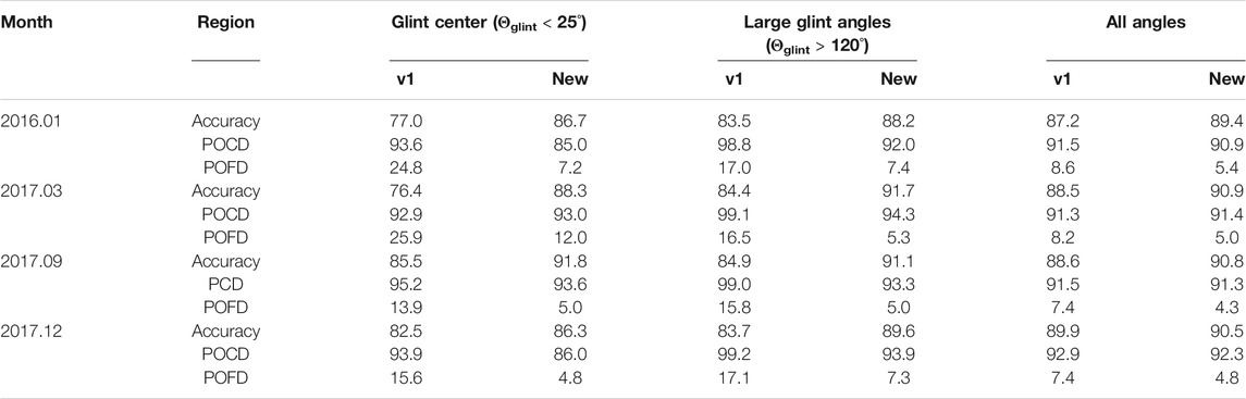
TABLE 2. Comparison of EPIC ocean cloud mask performance between the Version 2 algorithm and the new algorithm at glint center (Θglint < 25°), large glint angles (Θglint > 120°), and all glint angles of four additional months.
Systematic retrieval bias can often be revealed through examining the retrieved parameters as a function of independent variables such as viewing geometry (Zhou et al., 2020). During the evaluation of the EPIC cloud products, we notice that the EPIC clear and cloud detection rates vary with view zenith angle. Here the clear (cloud) detection rates are computed as the number of matched clear (cloudy) pixels divided by total clear (cloudy) pixels.
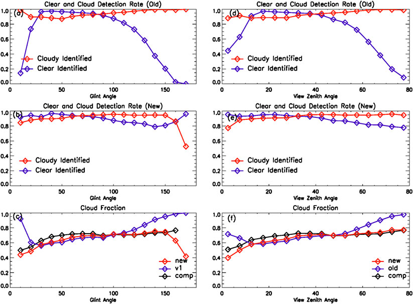
FIGURE 9. Comparison of cloud (red) and clear (blue) detection rates as a function of glint angle from Version 2 algorithm (A) and the new algorithm (B). (C) cloud fraction as a function of glint angle from GEO/LEO composite (black line), Version 2 algorithm (blue) and the new algorithm (red). (E–F) are similar as (A–C) except as a function of view zenith angles. Data are from January and July of 2017.
As mentioned in Glint distributions and impact, sunglint affects a zonal band of 30° in any given time of the year in tropical regions from 38°S to 38°N. Since sunglint appears near the centers of the granules which correspond to local noon time, it is likely that tropical oceanic cloud diurnal cycle analysis is affected if sunglint is not properly treated. In addition, a fixed threshold would misidentify pixels near granule edges to be cloudy because of high reflectance in those areas.
In Figure 10 we examine the latitudinal distributions of daytime cycles of cloud fraction over oceans in January and July. Note the complete diurnal cycle is not available from EPIC since it only measures the sunlit side of the Earth. The daytime cycle is computed by first converting the cloud mask retrievals from universal time (UTC) to local time according to their longitudes and then sorting the pixels according to their local solar time and latitude bins. Mean cloud fraction is then computed based on cloud mask results for each of these bins. Because the length of daytime differs with latitude, the figures are bell-shaped toward the winter hemisphere (shorter daytime in the winter hemisphere). One feature of the old latitudinal distribution of daytime cloud cycles is the circle-shaped high values in the midst of low cloud fraction near 20°S in January and 20°N in July at local noon, corresponding to glint center latitude in these two months (Figures 10A,E). The new algorithm has largely eliminated this artificial noon peak in the daytime cloud fraction (Figures 10B,F). In addition, the old cloud mask has produced near 100% cloud fraction in the beginning and ending hours of the daylight time even in dry subtropical latitudes, which is due to high-reflectance at large zenith angles. This problem is largely mitigated in the new algorithm. The difference maps clearly show reduced cloud fraction in the glint center and daytime edge hours (Figures 10C,G). This is especially significant in the glint center latitudes (Figures 10D,H), because 1) the noon peak disappears, and 2) even though diurnal cycle still features as higher cloud fraction in the morning and afternoon with minimum in local noon, the range of daytime cloud variation is greatly reduced.
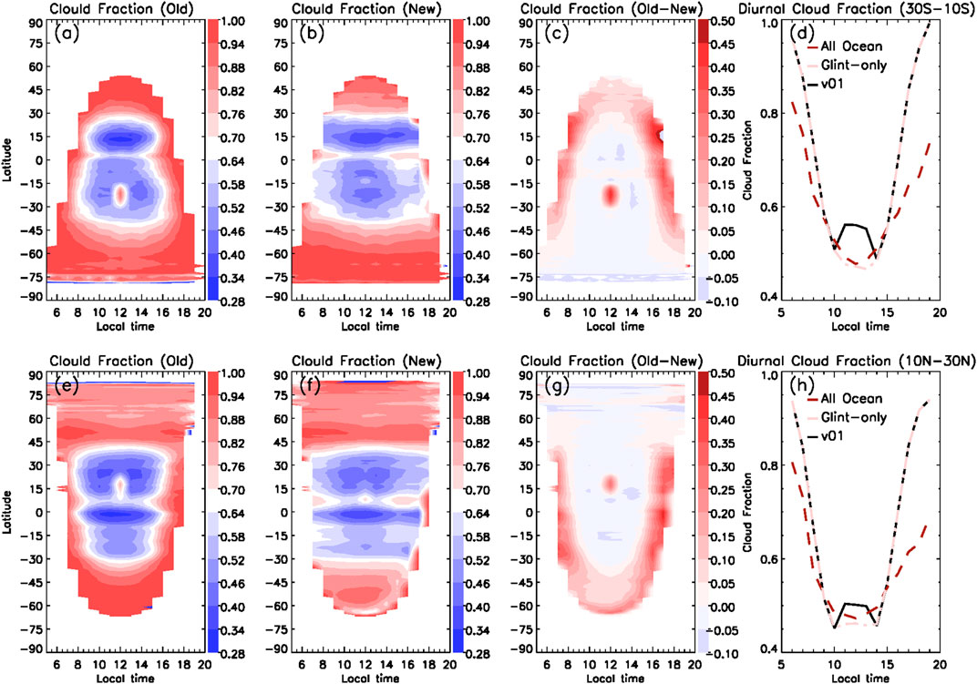
FIGURE 10. Zonal mean oceanic cloud fraction as a function of latitude and local time from the old algorithm (A,E), the new algorithm (B,F) and the difference (old–new) (C,G) in January (top) and July (bottom) in 2016. (D,H) show daytime cycle of cloud fractions from glint center latitudes (10°S–30°S) in January and (10°N–30°N) in July, respectively.
Because of the reduction in cloud fraction in the glint center and granule edge, some reduction in the zonal mean oceanic cloud fraction is expected. Figure 11 shows that the reduction appears for different latitudes in different seasons. In January, glint related reduction of about 10% appears around 25°S and up to 10% north of 15°N (Figure 11A). In July, the opposite is observed even though glint related reduction is smaller near 25°N (Figure 11C). In March and September, the Sun is near the equator; therefore, major reductions of cloud fraction occur in the latitudinal zone of 15°S–15°N, and high latitudes in each hemisphere also incur less reduction.
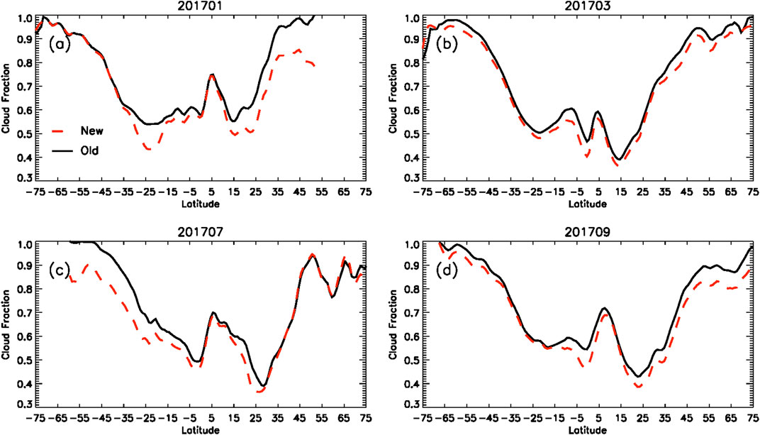
FIGURE 11. Zonal mean oceanic cloud fraction with latitude from old cloud mask algorithm (black) and new algorithm (red) in January, March, July, and September 2017.
Even though the old EPIC cloud mask algorithm attempts to reduce the sun-view geometry impact by applying the Rayleigh correction procedure, it is shown that fixed thresholds with the visible and near infrared channels lead to biases in the EPIC cloud mask product. Because of EPIC’s unique orbit, each EPIC granule over the ocean consists of a large area near the granule center that is affected by the sunglint. The glint affected area covers a latitudinal band of about 30° at any given time and migrates between 38°S and 38°N as the direct Sun position moves with the season. The old EPIC cloud mask tends to miss-identify the clear sunglint pixels as cloud due to its fixed reflectance threshold, therefore creating an artificial cloud fraction peak in local noon time. In addition, pixels with large Sun and view zenith angle at the granule edge tend to be miss-identified as clouds because of enhanced Rayleigh scattering.
A new ocean cloud mask algorithm is developed, which consists of two tests. The first test is based on the Rayleigh corrected 780 nm reflectance. A dynamic threshold dataset is developed as a function of glint angle to account for the enhanced reflectance in the glint region at the granule center and large glint angle region at the granule edge. The second test is based on the O2 A-band ratio, which is applied to regions where glint angles are smaller than 25o. Inside the sunglint region, the cloudy sky 780 nm reflectance can be smaller than that of the clear sky when clouds are thin. A unique property of A-band ratio is that the clear sky A-band ratio is lower than that of the cloudy A-band ratio in the glint center; thus, a supplemental A-band ratio test in the Sun glint regions can make up the reflectance test. The consistency of the new ocean cloud mask algorithm, as compared with GEO/LEO cloud detection, has increased by 4∼10% and 4∼6%, in the glint center and granule edges respectively. The false cloud detection rate is reduced by 10∼17% and the overall global ocean cloud detection consistency is increases by approximately 2%. The new algorithm has largely eliminated the systematic biases dependent on glint-angle and view zenith angles found in the old algorithm.
The new ocean cloud mask algorithm can help studies on the diurnal cycles of cloud fraction over ocean by reducing the artificial peak at local noon time in the glint center latitudes and by reducing early morning and late afternoon cloud fraction biases.
The datasets presented in this study can be found in online repositories. The names of the repository/repositories and accession number(s) can be found below: https://asdc.larc.nasa.gov/project/DSCOVR/DSCOVR_EPIC_L2_CLOUD_03.
YZ designed the new improvements of the ocean cloud mask algorithm, conducted the analysis and drafted the paper. YY led the development of the EPIC cloud algorithm, contributed to the design, testing and implementation of the new improvements to the operational algorithm. MG and P-WZ conducted the EPIC simulations and analysis. All authors contributed to the writing of the manuscripts.
The authors declare that the research was conducted in the absence of any commercial or financial relationships that could be construed as a potential conflict of interest.
Ackerman, S., Strabala, K., Menzel, P., Frey, R., Moeller, C., and Gumley, L. (2010). “Discriminating clear-sky from Cloud with MODIS Algorithm Theoretical Basis Document (MOD35),” in MODIS Cloud Mask Team, Cooperative Institute for Meteorological Satellite Studies (Madison: University of Wisconsin).
Barker, H. W., Stephens, G. L., Partain, P. T., Bergman, J. W., Bonnel, B., Campana, K., et al. (2003). Assessing 1D Atmospheric Solar Radiative Transfer Models: Interpretation and Handling of Unresolved Clouds. J. Clim. 16, 2676–2699. doi:10.1175/1520-0442(2003)016<2676:adasrt>2.0.co;2
Buehler, S. A., Eriksson, P., and Lemke, O. (2011). Absorption Lookup Tables in the Radiative Transfer Model ARTS. J. Quantitative Spectrosc. Radiative Transfer 112 (10), 1559–1567. doi:10.1016/j.jqsrt.2011.03.008
Cox, C., and Munk, W. (1954a). Measurement of the Roughness of the Sea Surface from Photographs of the Sun's Glitter. J. Opt. Soc. Am. 44, 838–850. doi:10.1364/josa.44.000838
Cox, C., and Munk, W. (1954b). Statistics of the Sea Surface Derived from Sun Glitter. J. Mar. Res. 13, 198–227.
Davis, A. B., Ferlay, N., Libois, Q., Marshak, A., Yang, Y., and Min, Q. (2018b). Cloud Information Content in EPIC/DSCOVR's Oxygen A- and B-Band Channels: A Physics-Based Approach. J. Quantitative Spectrosc. Radiative Transfer 220, 84–96. doi:10.1016/j.jqsrt.2018.09.006
Davis, A. B., Merlin, G., Cornet, C., Labonnote, L. C., Riédi, J., Ferlay, N., et al. (2018a). Cloud Information Content in EPIC/DSCOVR's Oxygen A- and B-Band Channels: An Optimal Estimation Approach. J. Quantitative Spectrosc. Radiative Transfer 216, 6–16. doi:10.1016/j.jqsrt.2018.05.007
Delgado‐Bonal, A., Marshak, A., Yang, Y., and Oreopoulos, L. (2020). Daytime Variability of Cloud Fraction from DSCOVR/EPIC Observations. J. Geophys. Res. Atmos. 125 (10). doi:10.1029/2019JD031488
Ding, S., Wang, J., and Xu, X. (2016). Polarimetric Remote Sensing in Oxygen A and B Bands: Sensitivity Study and Information Content Analysis for Vertical Profile of Aerosols. Atmos. Meas. Tech. 9, 2077–2092. doi:10.5194/amt-9-2077-2016
Ferlay, N., Thieuleux, F., Cornet, C., Davis, A. B., Dubuisson, P., Ducos, F., et al. (2010). Toward New Inferences about Cloud Structures from Multidirectional Measurements in the Oxygen A Band: Middle-Of-Cloud Pressure and Cloud Geometrical Thickness from POLDER-3/PARASOL. J. Appl. Meteorol. Climatol. 49, 2492–2507. doi:10.1175/2010JAMC2550.1
Fischer, J., and Grassl, H. (1991). Detection of Cloud-Top Height from Backscattered Radiances within the Oxygen A Band. Part 1: Theoretical Study. J. Appl. Meteorol. 30, 1245–1259. doi:10.1175/1520-0450(1991)030<1245:docthf>2.0.co;2
Frey, R. A., Ackerman, S. A., Liu, Y., Strabala, K. I., Zhang, H., Key, J. R., et al. (2008). Cloud Detection with MODIS. Part I: Improvements in the MODIS Cloud Mask for Collection 5. J. Atmos. Oceanic Technol. 25, 1057–1072. doi:10.1175/2008JTECHA1052.1
Gao, M., Zhai, P.-W., Yang, Y., and Hu, Y. (2019). Cloud Remote Sensing with EPIC/DSCOVR Observations: a Sensitivity Study with Radiative Transfer Simulations. J. Quantitative Spectrosc. Radiative Transfer 230, 56–60. doi:10.1016/j.jqsrt.2019.03.022
Hagolle, O., Nicolas, J.-M., Fougnie, B., Cabot, F., and Henry, P. (2004). Absolute Calibration of VEGETATION Derived from an Interband Method Based on the Sun Glint over Ocean. IEEE Trans. Geosci. Remote Sensing 42 (7), 1472–1481. doi:10.1109/TGRS.2004.826805
Harmel, T., and Chami, M. (2013). Estimation of the Sunglint Radiance Field from Optical Satellite Imagery over Open Ocean: Multidirectional Approach and Polarization Aspects. J. Geophys. Res. Oceans 118, 76–90. doi:10.1029/2012JC008221
Jackson, C. R., and Alpers, W. (2010). The Role of the Critical Angle in Brightness Reversals on Sunglint Images of the Sea Surface. J. Geophys. Res. 115, C09019. doi:10.1029/2009JC006037
Kay, S., Hedley, J., and Lavender, S. (2009). Sun Glint Correction of High and Low Spatial Resolution Images of Aquatic Scenes: a Review of Methods for Visible and Near-Infrared Wavelengths. Remote Sensing 1, 697–730. doi:10.3390/rs1040697
Khattak, S., Vaughan, R., and Cracknell, A. (1991). Sunglint and its Observation in AVHRR Data. Remote Sensing Environ. 37 (2), 101–116. doi:10.1016/0034-4257(91)90022-X
Khlopenkov, K. V., Su, W., Duda, D. P., Minnis, P., Bedka, K. M., and Thieman, M. (2017). “Development of Multi-Sensor Global Cloud and Radiance Composites for Earth Radiation Budget Monitoring from DSCOVR,” in Proceedings Volume 10424, Remote Sensing of Clouds and the Atmosphere XXII (Warsaw, Poland: SPIE Remote Sensing), 104240K. doi:10.1117/12.2278645
Levy, R. C., Remer, L. A., Martins, J. V., Kaufman, Y. J., Plana-Fattori, A., Redemann, J., et al. (2005). Evaluation of the MODIS Aerosol Retrievals over Ocean and Land during CLAMS. J. Atmos. Sci. 62, 974–992. doi:10.1175/JAS3391.1
Marshak, A., Herman, J., Adam, S., Karin, B., Carn, S., Cede, A., et al. (2018). Earth Observations from DSCOVR EPIC Instrument. Bull. Amer. Meteorol. Soc. 99 (9), 1829–1850. doi:10.1175/BAMS-D-17-0223.1
Meyer, K., Yang, Y., and Platnick, S. (2016). Uncertainties in Cloud Phase and Optical Thickness Retrievals from the Earth Polychromatic Imaging Camera (EPIC). Atmos. Meas. Tech. 9, 1785–1797. doi:10.5194/amt-9-1785-2016
Minnis, P., Sun-Mack, S., Young, D. F., Heck, P. W., Garber, D. P., Chen, Y., et al. (2011). CERES Edition-2 Cloud Property Retrievals Using TRMM VIRS and Terra and Aqua MODIS Data-Part I: Algorithms. IEEE Trans. Geosci. Remote Sensing 49, 4374–4400. doi:10.1109/TGRS.2011.2144601
Ottaviani, M., Spurr, R., Stamnes, K., Li, W., Su, W., and Wiscombe, W. (2008). Improving the Description of Sunglint for Accurate Prediction of Remotely Sensed Radiances. J. Quantitative Spectrosc. Radiative Transfer 109, 2364–2375. doi:10.1016/j.jqsrt.2008.05.012
Richardson, M., Lebsock, M. D., McDuffie, J., and Stephens, G. L. (2020). A New Orbiting Carbon Observatory 2 Cloud Flagging Method and Rapid Retrieval of marine Boundary Layer Cloud Properties. Atmos. Meas. Tech. 13, 4947–4961. doi:10.5194/amt-13-4947-2020
Rothman, L. S., Gordon, I. E., Babikov, Y., Barbe, A., Chris Benner, D., Bernath, P. F., et al. (2013). The Hitran2012 Molecular Spectroscopic Database. J. Quantitative Spectrosc. Radiative Transfer 130, 4–50. doi:10.1016/j.jqsrt.2013.07.002
Stammes, P., Sneep, M., de Haan, J. F., Veefkind, J. P., Wang, P., and Levelt, P. F. (2008). Effective Cloud Fractions from the Ozone Monitoring Instrument: Theoretical Framework and Validation. J. Geophys. Res. 113, D16S38. doi:10.1029/2007JD008820
Su, W., Liang, L., Doelling, D. R., Minnis, P., Duda, D. P., Khlopenkov, K., et al. (2018). Determining the Shortwave Radiative Flux from Earth Polychromatic Imaging Camera. J. Geophys. Res. Atmos. 123, 11479–11491. doi:10.1029/2018JD029390
Wang, P., Stammes, P., van der A, R., Pinardi, G., and van Roozendael, M. (2008). FRESCO+: an Improved O2 A-Band Cloud Retrieval Algorithm for Tropospheric Trace Gas Retrievals. Atmos. Chem. Phys. 8, 6565–6576. doi:10.5194/acp-8-6565-2008
Yang, Y., Marshak, A., Chiu, J. C., Wiscombe, W. J., Palm, S. P., Davis, A. B., et al. (2008). Retrievals of Thick Cloud Optical Depth from the Geoscience Laser Altimeter System (GLAS) by Calibration of Solar Background Signal. J. Atmos. Sci. 65 (11), 3513–3526. doi:10.1175/2008JAS2744.1
Yang, Y., Marshak, A., Mao, J., Lyapustin, A., and Herman, J. (2013). A Method of Retrieving Cloud Top Height and Cloud Geometrical Thickness with Oxygen A and B Bands for the Deep Space Climate Observatory (DSCOVR) Mission: Radiative Transfer Simulations. J. Quantitative Spectrosc. Radiative Transfer 122, 141–149. doi:10.1016/j.jqsrt.2012.09.017
Yang, Y., Meyer, K., Wind, G., Zhou, Y., Marshak, A., Platnick, S., et al. (2019). Cloud Products from the Earth Polychromatic Imaging Camera (EPIC): Algorithms and Initial Evaluation. Atmos. Meas. Tech. 12, 2019–2031. doi:10.5194/amt-12-2019-2019
Yin, B., Min, Q., Morgan, E., Yang, Y., Marshak, A., and Davis, A. B. (2020). Cloud-top Pressure Retrieval with DSCOVR EPIC Oxygen A- and B-Band Observations. Atmos. Meas. Tech. 13, 5259–5275. doi:10.5194/amt-13-5259-2020
Zhai, P.-W., Hu, Y., Chowdhary, J., Trepte, C. R., Lucker, P. L., and Josset, D. B. (2010). A Vector Radiative Transfer Model for Coupled Atmosphere and Ocean Systems with a Rough Interface. J. Quantitative Spectrosc. Radiative Transfer 111, 1025–1040. doi:10.1016/j.jqsrt.2009.12.005
Zhai, P.-W., Hu, Y., Trepte, C. R., and Lucker, P. L. (2009). A Vector Radiative Transfer Model for Coupled Atmosphere and Ocean Systems Based on Successive Order of Scattering Method. Opt. Express 17, 2057–2079. doi:10.1364/oe.17.002057
Zhou, Y., Yang, Y., Gao, M., and Zhai, P.-W. (2020). Cloud Detection over Snow and Ice with Oxygen A- and B-Band Observations from the Earth Polychromatic Imaging Camera (EPIC). Atmos. Meas. Tech. 13, 1575–1591. doi:10.5194/amt-13-1575-2020
Keywords: EPIC, cloud detection, sunglint, oxygen A-band, ocean surface reflectance
Citation: Zhou Y, Yang Y, Zhai P-W and Gao M (2021) Cloud Detection Over Sunglint Regions With Observations From the Earth Polychromatic Imaging Camera. Front. Remote Sens. 2:690010. doi: 10.3389/frsen.2021.690010
Received: 01 April 2021; Accepted: 09 June 2021;
Published: 15 July 2021.
Edited by:
Gregory Schuster, National Aeronautics and Space Administration, United StatesReviewed by:
Weizhen Hou, Aerospace Information Research Institute (CAS), ChinaCopyright © 2021 Zhou, Yang, Zhai and Gao. This is an open-access article distributed under the terms of the Creative Commons Attribution License (CC BY). The use, distribution or reproduction in other forums is permitted, provided the original author(s) and the copyright owner(s) are credited and that the original publication in this journal is cited, in accordance with accepted academic practice. No use, distribution or reproduction is permitted which does not comply with these terms.
*Correspondence: Yaping Zhou, eWFwaW5nLnpob3UtMUBuYXNhLmdvdg==
Disclaimer: All claims expressed in this article are solely those of the authors and do not necessarily represent those of their affiliated organizations, or those of the publisher, the editors and the reviewers. Any product that may be evaluated in this article or claim that may be made by its manufacturer is not guaranteed or endorsed by the publisher.
Research integrity at Frontiers
Learn more about the work of our research integrity team to safeguard the quality of each article we publish.