 Igor V. Geogdzhayev
 Alexander Marshak
 Mikhail Alexandrov1,2
- 1Department of Applied Physics and Applied Mathematics, Columbia University, New York, NY, United States
- 2NASA Goddard Institute for Space Studies, New York, NY, United States
- 3NASA Goddard Space Flight Center, Greenbelt, MD, United States
The first five years of operation of the Deep Space Climate Observatory (DSCOVR) Earth Polychromatic Imaging Camera (EPIC) at the Lagrange one point have produced results that uniquely complement the data from currently operating low orbit Earth-observing instruments. In this paper we describe an updated unified approach to EPIC calibration. In this approach, calibration coefficients and their trends were obtained by comparing EPIC observations to the measurements from polar orbiting radiometers. In this study L1B reflectances from Moderate Resolution Imaging Spectroradiometer (MODIS) onboard the Aqua and Terra satellites, Multi-angle Imaging Spectroradiometer (MISR) onboard Terra and Visible Infrared Imaging Radiometer (VIIRS) onboard the Suomi National Polar-orbiting Partnership (Suomi NPP) spacecraft were used to infer calibration coefficients for four EPIC visible and near-infrared channels: 443 nm, 551 nm, 680 nm, and 780 nm. EPIC Version three measurements made between June 2015 and August 2020 were used for comparison. The calibration procedure identifies the most homogeneous low Earth orbit radiometer scenes matching scattering angles that are temporarily and spatially collocated with EPIC observations. These scenes are used to determine reflectance to count (R/C) ratios in spectrally analogous channels. Seasonal average R/C ratios were analyzed to obtain EPIC calibration gains and trends. The trends for the full dataset period are not statistically significant except in the 443 nm channel. No significant changes in calibration were found after the instrument’s exit from safe hold in March 2020. The R/C ratios were also used to determine the differences in EPIC gains resulting from separate calibrations: against MODIS Aqua or Terra, as well as against forward or aftward MISR cameras. Statistical tests indicate that the differences between the two datasets are not significant except in the 780 nm channels where Aqua-derived coefficients may be around 2% lower compared to Terra. The dependence of EPIC calibration gains on the instrument scattering angle and on DSCOVR-Earth distance were investigated. Lastly, model Low Earth Orbit (LEO) reflectances calculated to match the EPIC viewing geometry were employed to study how EPIC calibration coefficients depend on EPIC-LEO viewing geometry differences. The effect of LEO and EPIC angular mismatch on calibration was shown to be small.
Introduction
The Deep Space Climate Observatory (DSCOVR) spacecraft actively maintains itself in a Lissajous orbit around the Lagrange point L1 between the Sun and the Earth at about 1.5 million kilometers from Earth (Marshak et al., 2018). From this position the DSCOVR Earth Polychromatic Imaging Camera (EPIC) views the entire sunlit Earth’s hemisphere in ten narrow spectral channels ranging from UV to near IR 10 (in winter) to 22 (in summer) times a day. The Earth-observing geometry of the EPIC instrument is close to backscattering: the scattering angle varies between 168 and 178°. EPIC’s viewing geometry differs significantly from instruments on sun-synchronous orbits for which only a small portion of Earth views occurs in the backscattering region. For comparison, depending on the season, latitude and scan view angle, the scattering angle for MODIS is typically in a wide range between 110 and 175°. The Suomi-NPP VIIRS instrument, due to its wider scan, covers an even larger range of angles, including the whole backscattering region. The near-backscattering EPIC observations are a direct consequence of its position at L1.
We previously reported Geogdzhayev and Marshak, (2018) EPIC calibration coefficients based on comparisons with MODIS. Since then, Version 3 EPIC L1b data has become available. Compared to Version 2, significant improvements were made in geolocation and flatfield correction (Kostinski et al., 2021). A number of L2 products were developed from EPIC observations. In this paper we describe an improved, more robust version of the intercalibration algorithm and apply it to data from four low Earth orbit (LEO) radiometers. In addition, we analyze trends and sources of variability in the derived calibration.
Thanks to its unique vantage point and spatial and temporal Earth coverage, EPIC remote sensing observations have been used in such applications as the retrieval of aerosol, cloud, sulfur dioxide and ozone amounts and vegetation properties Marshak et al., (2018), as well as ocean color products (Gao et al., 2019). In addition, EPIC data have been employed to observe volcanic clouds Carn et al. (2016, 2018), analyze the global distribution of erythemal irradiance Herman et al. (2020); Herman et al. (2018a), and observe solar eclipse irradiance changes (Herman at al., 2018b). EPIC observations in the backscattering region have been used to observe and characterize the glint caused by oriented ice crystals in clouds Varnai et al. (2020); Marshak et al. (2017), retrieve cloud properties Yang et al. (2013); Yang et al. (2019); Yin et al. (2020), ozone Herman et al. (2018a) and vegetation properties (Marshak et al., 2017; Yang et al., 2017). More EPIC-related research papers may be found here: https://epic.gsfc.nasa.gov/science/pubs.
Most of the above applications rely on radiometric calibration of the EPIC measurements. The lack of in-flight calibration capabilities necessitates a comparison of EPIC Earth observations with well-calibrated measurements from radiometers in polar and geostationary orbits. In addition, the images of the Moon regularly observed by the instrument may also be employed for calibration.
In this study we employ EPIC measurements combined with collocated Level 1b TOA reflectances from the Moderate Resolution Imaging Spectroradiometer King et al. (2003) on-board the Aqua and Terra satellites, the Multi-angle Imaging Spectroradiometer Diner et al. (2005) on-board Terra and the Visible Infrared Imaging Radiometer Suite Cao et al. (2014), which is part of the Suomi National Polar-orbiting Partnership (NPP), to derive the calibration coefficients in four EPIC visible and near-infrared (NIR) channels. These instruments were chosen for comparison because of their well-established calibration record and wide use in the remote sensing applications. Contemporaneous data from these instruments are available for the entire period of the DSCOVR mission. Using these data, we derive calibration gains for the latest Version 3 release of the EPIC data.
Data
Version 3 data EPIC L1B data were obtained from the NASA EOSDIS OpeNDAP data server at https://opendap.larc.nasa.gov/opendap/. The EPIC sampling size at nadir (at the center of the image) is about 8 km × 8 km (10 km × 10 km when the EPIC point spread function is applied) and increases toward the edges. The radiometric resolution of the EPIC data is 12 bits per pixel. To reduce the amount of data transmitted from DSCOVR, for all but the blue channel (443 nm), four pixels are averaged on-board the spacecraft resulting in an effective spatial resolution at nadir of approximately 18 km.
We use MODIS Aqua and Terra L1B Collection 6.1 1 km reflectances obtained from the Level-1 and Atmosphere Archive and Distribution System (LAADS) Distributed Active Archive Center (DAAC). Note that the MODIS reflectance, as well as the EPIC one, is the true TOA reflectance multiplied by the solar zenith angle (MODIS Characterization Support Team, 2006). We will refer to this quantity simply as “reflectance” and will use it for all radiometers. MODIS also has a radiometric resolution of 12 bits per pixel and calibration design requirements of 2% for reflectance and 5% for radiance in the solar bands (Toller et al., 2013). MODIS instruments have a cross-track swath width of 2,330 km. The equator crossing times are 10:30 AM and 1:30 PM for MODIS Terra and Aqua, respectively. We note here that while we used publicly available MODIS L1B data obtained from LAADS DAAC, additional calibration for Terra and Aqua is performed in MODIS Land discipline processing. This additional calibration includes polarization correction of Terra data based on Ocean Biology Processing Group Kwiatkowska et al. (2008), de-trending for both Terra and Aqua, and gain adjustment for Terra (cross-calibration to Aqua). These coefficients come from the Multi-Angle Implementation of Atmospheric Correction (MAIAC) group’s calibration over deserts sites (Lyapustin et al., 2014). This additional calibration was not used in this study.
The MISR ellipsoid-projected L1B2 radiance product (MI1B2E) data were obtained from the Atmospheric Science Data Center (ASDC) DAAC. MISR uses 14-bit quantization and has an instrument specification for radiometric accuracy of 3% at maximum signal (Bruegge et al., 2002). The global mode data are provided at 1.1 km spatial resolution for all nine cameras in blue (446 nm), green (558 nm), and NIR (866 nm) channels and for the nadir camera in the red (672 nm) channel. The off-nadir red channel data provided at 275 m resolution were downsampled to 1.1 km to match the other channels/cameras. MISR is onboard the Terra satellite and thus has identical equator crossing time as MODIS Terra. Among the LEO instruments considered in this paper it has the narrowest swath of 360 km in the cross-track direction.
The VIIRS Level 1 data were downloaded from the Level-1 and Atmosphere Archive and Distribution System (LAADS) DAAC. The moderate resolution (750 m) channels M3 (448 nm), M4 (555 nm), M5 (672 nm) and M7 (865 nm) were used in this study. VIIRS radiometric accuracy requirement is 2% in reflectance of a typical scene radiance (JPSS Level 1 Requirements Document, 2016). The VIIRS daytime equator crossing time is similar to MODIS Aqua, at 1:30 PM. The instrument is on a higher orbit compared to Terra and Aqua satellites and has a wide swath of 3,060 km, sufficient to eliminate data gaps from adjacent orbits in the tropics.
The matching of EPIC channels to those of the LEO instruments is summarized in Table 1. The table also includes the position and bandwidth of the channels.
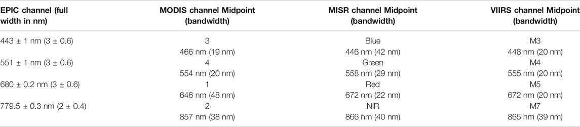
TABLE 1. EPIC-MODIS-MISR-VIIRS channel correspondence. Midpoint wavelengths are band-averaged values. For simplicity, for the rest of the paper we will call the EPIC NIR channel 780 nm.
Figure 1 compares the normalized filter functions of the four instruments to the corresponding EPIC channels. The curves for the matching channels are marked by the same color. As one can see from the figure, EPIC channels are significantly narrower compared to the channels of LEO radiometers. The best spectral match is for the overlapping green channels, while the largest spectral difference, of about 80 nm, is observed between the NIR channels. The central wavelength of the EPIC NIR channel is significantly shorter compared to the LEO radiometers. While the locations of the green and NIR spectral channels are similar among the LEO radiometers, there are differences in positions of the blue channels. Compared to MISR and VIIRS the red channel of MODIS is shifted toward the shorter wavelengths. We note that the spectral channels used for intercomparison in this study are not exhaustive. Other MODIS and VIIRS channels, such as VIIRS M6 (745 nm) and MODIS Band 15 (748 nm) ocean color bands in near IR, may be employed for this purpose.
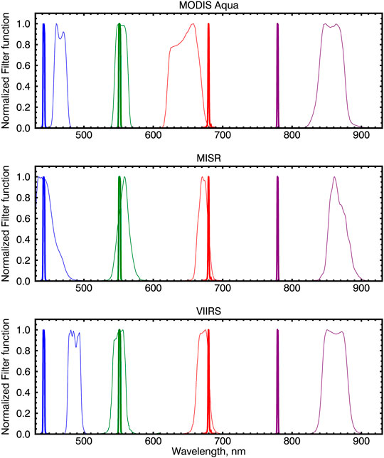
FIGURE 1. MODIS (upper panel), MISR (middle panel), VIIRS (lower panel) spectral response functions normalized to the maximum value for the channels used in this study are shown by wide curves. Repeated on each panel are the corresponding EPIC channels (narrow curves).
Methods
The first step for the derivation of EPIC calibration coefficients is to identify favorable LEO scenes. This process is illustrated by Figure 2 for MODIS (upper panel), MISR (middle panel) and VIIRS (lower panel). All EPIC observations are made in the backscattering region, while for the LEO instruments only a small fraction of the pixels have similar viewing geometry. We therefore begin by selecting pixels that match the EPIC scattering angle to within 1.5°. LEO radiometer pixels that satisfy this criterion form a ring on the Earth surface, shown as white areas in Figure 2. Compared to the EPIC Version 2 calibration approach Geogdzhayev and Marshak, (2018), the angular match threshold was relaxed to increase the number of matching fully filled scenes away from the ring borders. Due to the relatively narrow width of the MISR cross-track swath, matching areas are often found on the edge of the scan, as illustrated in the middle panel of Figure 2, where the dark area in the upper right part of the image is outside of the MISR swath. To mitigate this effect, the scattering angle matching threshold was relaxed to 3°. We ran tests using MODIS data to evaluate the effect of such a change and did not find it to be significant. Among the selected pixels, we retain those taken within 7 min of the EPIC image. These pixels are shown as dots in the white areas of the images of Figure 2. There are time lags in the data acquisition between different EPIC spectral channels associated with the rotation of the filter wheels: ∼3 min difference between blue (443 nm) and green (551 nm), and ∼4 min between blue and red (680 nm) (Marshak and Knyazikhin, 2017). Therefore, the temporal collocation is done separately for each spectral channel. The solar zenith angle (SZA) of all matching pixels is limited to 60° to exclude scenes with low illumination and scenes where the curvature of the Earth may complicate the comparison. Pixels within 40° of the glint angle over ocean are excluded as well. For each EPIC pixel that matches the above criteria we identify LEO radiometer pixels that fall within an approximately 25 km radius. Scenes are retained for further analysis if at least 2/3 of the 25 km neighborhood is covered with valid LEO radiometer pixels (one such scene is represented by a gray circle on each of the upper and lower panels of Figure 2). This requirement was introduced in the current version of the algorithm and serves to exclude sparsely populated scenes that can have more variability, thus introducing more noise in comparisons. For each matching scene we calculate the mean and relative standard deviation (defined as the ratio of the standard deviation to the mean) for the matching LEO radiometer pixels within the 25 km radius. We also calculate the standard deviation for the 5 × 5 EPIC pixel neighborhood. The values of the relative standard deviation are used to select the most homogeneous scenes.

FIGURE 2. Examples of matching EPIC-LEO instrument scenes. Top, middle and lower panels show selected areas of MODIS, MISR and VIIRS images (green channel reflectances), respectively. MODIS image is approximately 400 km in the cross-track dimension and 2,000 km long and is centered on 24.5°S and 51.1°E. MISR image is approximately 250 km in the cross-track dimension and 1,750 km long and cetered at 17.1°S and 141.61°E. VIIRS image is approximately 330 km in the cross-track dimension and 2,200 km long and cetered at 27.5°N and 43.9°E Areas of matching scattering angles are shown in white. Black dots on white are EPIC pixels that are temporarily and spatially collocated with LEO instrument pixels. Gray circles on the upper lower panel shows the 25 km vicinity of single EPIC pixels. Cross-track direction is approximately vertical. Dark upper-right region in the middle panel is outside of the MISR swath. White streaks on top of the lower panel are due to VIIRS bow-tie effect.
The differences in the position and spectral width of the corresponding EPIC and LEO radiometer channels illustrated in Figure 1 may cause discrepancy when a scene is observed by the two orbit types (Chander, 2013). This discrepancy is generally a function of the scene’s spectral signature and may result in both noise and systematic errors of calibration. As in the previous V2 calibration procedure, in this work we compensate for these differences by employing spectral band adjustment factors (SBAFs), which convert MODIS, MISR and VIIRS TOA reflectance values to equivalent EPIC reflectances for various surface types. These factors, in the form of linear regression coefficients, were obtained from the database available at https://cloudsgate2.larc.nasa.gov/cgi-bin/site/showdoc?mnemonic = SBAF; they are based on the analysis of the SCIAMACHY hyperspectral data for various surface targets and account for the differences in radiometer’s spectral response functions (Scarino et al., 2016).
In addition, we used the same source to identify the range of reflectance values for each scene type. LEO radiometer’s pixels were adjusted if their reflectance was within this range using the SBAFs for the appropriate land cover type. For scenes with reflectance higher than 0.6 we used the deep convection cloud spectral corrections. Land cover types were taken from a data set developed by Channan et al. (2014). The dataset is a .5 x .5-degree reprojected version of the Global Mosaics of the standard MODIS land cover type data product (MCD12Q1) in the IGBP Land Cover Type Classification. Separate adjustment factors were used for each of the four LEO instruments.
The EPIC calibration coefficients may be derived from the matching scenes using two methods (Geogdzhayev and Marshak, 2018). The first one involves calculating the linear regression between EPIC counts/sec and LEO reflectances for the most homogeneous scenes. The second involves finding the mean reflectance/count (R/C) ratio for bright homogeneous scenes (LEO reflectance greater than 0.6). The two approaches possess a certain degree of independence since the regression method uses darker pixels in addition to the bright ones. A linear regression also produces the intercept values; their closeness to zero may be used as an indication of the quality of fit. The ratio method can be used on a smaller dataset to derive, for example, seasonal gains, or to investigate the sensitivity of calibration to various parameters. Since these topics will mostly be the focus of this study, here we will be using the ratio method.
Specifically, to derive calibration gains we employ the ratios of LEO instrument reflectance to EPIC count for all available matching scenes where the reflectance is greater than 0.6 and relative standard deviation is less than 10%. These scenes are binned according to the relative standard deviation of the MODIS reflectance and the mean R/C ratio is calculated for each bin. The mean bin values are then extrapolated to the ideal case of a completely uniform scene (zero standard deviation) using a linear regression. The extrapolated value is then taken to be the calibration coefficient.
The following list summarizes the conditions used to match pixels between EPIC and LEO instruments: 1) scattering angle is within 1.5° of the EPIC scattering angle 2) temporal collocation with EPIC image is less than 7 min for each EPIC channel 3) glint angle is greater than 40° 4) at least 2/3 of the 25 km-neighborhood of the EPIC pixel is covered with LEO radiometer measurements 5) LEO radiometer reflectance is greater than 0.6 6) relative standard deviation in the neighborhood is less than 10%.
Results
Calibration Gains and Trends
Figure 3 presents a summary of the calibration datasets as timeseries of seasonal mean R/C ratio for the four channels. The top, middle and lower panels show the combined MODIS Aqua and Terra data, MISR, and VIIRS NPP data, respectively. The gap in data in June 2019–February 2020 corresponds to the period when EPIC was is safe mode. The average number of points per year that went into the calculation of the curves on Figure 3 are 6,000 for MODIS, 70,000 for MISR and 20,000 for VIIRS. The higher value for MISR is due to the relaxed scattering angle match condition. The higher resolution and wider swath of VIIRS resulted in more matches compared to MODIS. The corresponding calibration gain values and their relative differences are given in Table 2. The values in Table 2 are based on the data for the time period to 06/2019, when EPIC was put in safehold. Encouragingly, MODIS results agree to within 1.4%, 0%, 1.2%, 2.6% with the corresponding values for each channel derived by an independent method by Doelling et al. (2019), also see (Haney et al., 2016). VIIRS results agree to within 0.4% with corresponding values from the same source. We found that the relative difference between calibration gains derived from MISR and VIIRS is less than 2% in all channels (last column in Table 2), while the MODIS-VIIRS difference is within 4.3%. These differences are in line with the reported values for the radiometric accuracy of the instruments.
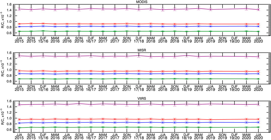
FIGURE 3. Time series of seasonal mean R/C ratios for combined MODIS Aqua and Terra instruments (upper panel), MISR (middle panel) and VIIRS (lower panel). Here and in the following R/C figures blue green, red and magenta lines represent 443, 551,680 and 780 nm EPIC channels. Whiskers represent the standard deviation of R/C ratios within each three-month period.

TABLE 2. EPIC calibration gains derived from several LEO instruments and their relative differences.
MODIS channel 2 may saturate over bright deep convective clouds (Doelling et al., 2019). In this study we considered MODIS L1B data marked to be within the valid range (integer values [0, 32,767]). The saturated pixels (with value 65,533) were excluded. To investigate whether possible saturation of MODIS band 2 affected our results, we recalculated the 780 nm calibration gain while additionally restricting MODIS reflectances to values smaller than some threshold. Across all threshold values down to 0.7, we found that the effect on the calibration was limited to about 0.5%.
We used the seasonal mean R/C values summarized in Figure 3 to estimate calibration gain trends for the whole period of EPIC data. The results are listed in Table 3. As can be seen from the table, EPIC calibration values are stable. We used a standard double-sided test with a 95% confidence threshold (corresponding to a “p-value” of 0.05) to evaluate the statistical significance of the trends. We found the calculated trend values to not be statistically significant (with corresponding p-values greater than 0.05), except in the blue channel for VIIRS data. To test how the resumption of operations in March 2020 affected the calibration, we used the trend values from Table 3 together with their confidence intervals to find the expected range of R/C values for the two 3 month periods after the gap (the last two points of the curves in Figure 3). We found that the actual values are well within the expected range for all instruments. We conclude that the safe hold incident did not noticeably affect the calibration.
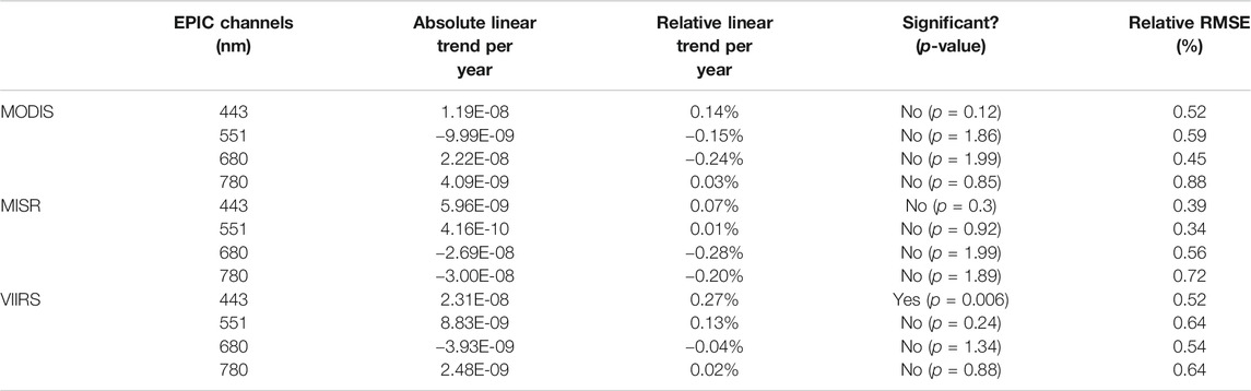
TABLE 3. Absolute and relative EPIC calibration gains trends derived from several LEO instruments and their statistical significance.
Next, we normalized the time series for MODIS, MISR and VIIRS to the second three-month period (September-October-November of 2015) and combined them into one time series by taking the arithmetic average of the three curves as illustrated in Figure 4, since the first three-month period (June-July-August 2015) contains fewer EPIC data points leading to more variability in the calculated values. Using this combined time-series we calculated the “overall” MODIS + MISR + VIIRS trends. The values are shown on the inserts in Figure 4. We found a small statistically significant trend of 0.16%/year in the 443 nm channel, while trends in other channels were not significant. The differences between the normalized curves (gray lines) appear to be greater in the red and NIR channels compared to the blue and green channels. It can be seen from the last column of Table 3 that relative RMSE values are higher in the NIR channels compared to the visible channels for all LEO instruments, possibly due to bigger spectral separation (see Figure 1). This may have contributed to the larger differences for the 780 nm curves. In addition, the observed offsets between individual instrument curves may partly be an artifact of random differences between the instruments at the point of normalization. This, however, does not have any effect on the trend calculations.
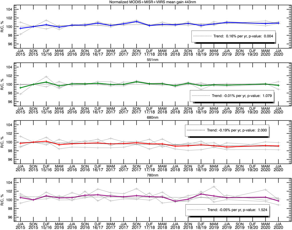
FIGURE 4. Average MODIS + MISR + VIIRS seasonal mean R/C values normalized to one on SON 2015 (colored curves). Solid gray curves are for individual LEO instruments, dotted line is linear trend.
Variability due to Orbital Motion
The DSCOVR satellite’s orbital motion around L1 point means that EPIC’s scattering angle fluctuates by as much as 10° in the time frame of about 1.5°months (top panel of Figure 5). In addition, the instrument’s distance to Earth can change by as much 200,000 km in about 3°months (top panel of Figure 6). This behavior differs a lot form the very regular orbits of instruments in sun-synchronous or geostationary orbits. In this section we estimate how much variability in EPIC calibration is caused by the DSCOVR orbital motion. This is useful for algorithm validation and provides reference values for EPIC-LEO intercalibration and trend analysis. Detrended R/C ratios derived from MODIS were binned and averaged according to the EPIC scattering angle and according to the EPIC-Earth distance. The results are displayed on the lower panels of Figures 5, 6. The dependance of the R/C ratios on the scattering angle is essentially flat with some increase observed for the largest angles in the 443 and 680 nm channels. RMSE values over the four bins used is about 1%. We conclude that the changes in scattering angle are not a significant source of variability of the calibration gains. The changes in the DSCOVR-Earth distance have an even smaller effect on the variability of calibration values, as can be seen from the lower panel of Figure 6. The corresponding RSME values are on the order of 0.5% for the binned R/C mean values. As expected, this value is small, because EPIC counts for identical scenes should not depend on the distance from Earth.
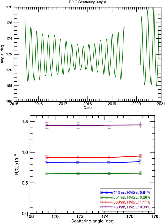
FIGURE 5. Top panel: EPIC scattering angle vs. time. Lower panel: mean R/C ratio vs. scattering angle. Whiskers represent the standard deviation of the values within each bin. Based on MODIS data.
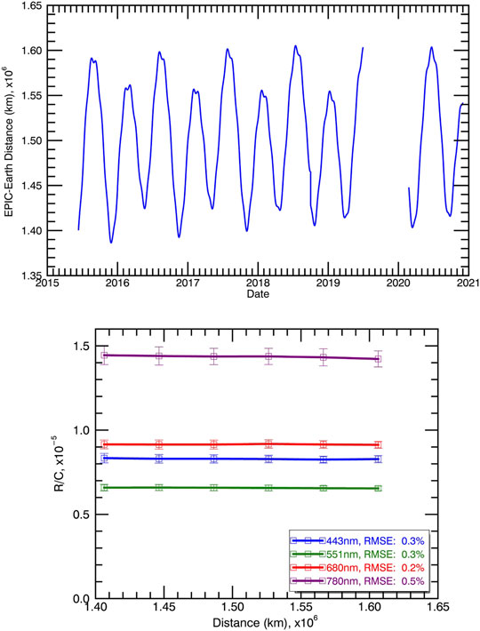
FIGURE 6. Top panel: EPIC-Earth distance vs. time. Lower panel: mean R/C ratio vs. EPIC-Earth distance. Whiskers represent the standard deviation of the values within each bin. Based on MODIS data.
Aqua- and Terra-Derived Calibration
In the preceding sections, data from MODIS Aqua and Terra were combined into one dataset. While the two instruments are very similar and follow the same calibration approach, the Aqua and Terra satellites have different equator crossing times and thus, generally speaking, different observational geometries. It is therefore of interest to investigate the differences that may occur if the two instruments are used separately. Figure 7 presents the time-series of R/C ratios derived from MODIS Terra (blue curve) and MODIS Aqua (red curve), while Table 4 lists the relevant statistics. We found that MODIS Aqua R/C values have higher variability compared to MODIS Terra (third and second columns of Table 4, respectively). Assuming that seasonal mean R/C values are statistically independent samples, we can apply the Kolmogorov-Smirnov (KS) test to the two datasets. The test reveals that the Terra and Aqua values for 443, 551 and 680 nm channels are not significantly different (the fifth column of Table 4). However, a significant statistical difference exists between Aqua- and Terra-derived 780 nm values, with Aqua values being systematically lower by about 2% compared to Terra. This is consistent with the higher (2.6%, see Calibration Gains and Trends above) difference in the calibration gains in this channel reported here and by Doelling et al. (2019), since they used MODIS Aqua data only. In addition, the Aqua 780 nm R/C ratios appear to be somewhat higher during the period from the middle of 2017 to the middle of 2018 than during other periods (Figure 7). We cannot establish with confidence the cause of these differences. We plan to investigate them further using the additional MODIS calibration from MODIS Land discipline processing, mentioned in Data, which does not have trends or biases between the two MODIS sensors. Please refer to Modeling Earth Polychromatic Imaging Camera Reflectances below for additional modeling analysis and further discussion.
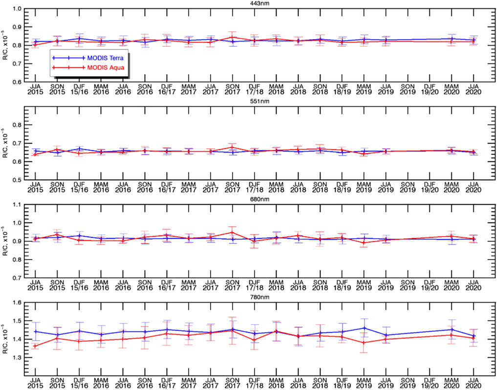
FIGURE 7. Time series of MODIS Aqua (red) and Terra (blue) derived seasonal mean R/C ratios.
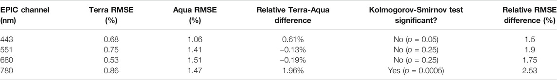
TABLE 4. Statistics of EPIC R/C ratios derived from Terra and Aqua MODIS data.
Multi-Angle Imaging Spectroradiometer Camera-Specific Calibration Analysis
MISR on board Terra spacecraft has a nadir, 4 forward, and 4 aftward looking cameras. Figure 8 shows the distribution of EPIC-matching pixels over MISR cameras. Over 80% of EPIC matches are viewed through the two cameras closest to nadir (Af and Aa). The number of matching pixels viewed through each of these cameras (around 40%) is similar across the four channels. Some variation may be due to time delays between EPIC image acquisition in different spectral channels. We can compare the calibration gains derived separately for the two cameras. The results of an analysis analogous to the previous section are summarized in Figure 9. We found the relative difference between the MISR aftward (Aa) and forward (Af) cameras to be 0.03, −0.02, −1.53, and −0.85% for the 443, 551, 680 and 780 nm channels, respectively. The corresponding relative RMSE differences were 1, 1, 1.7, and 1.4%. Using the Kolmogorov-Smirnov test, we determined that the differences between EPIC R/C values derived from the two MISR cameras’ data are not statistically significant in the blue and green channels (p-values of 0.5 and 0.3, respectively) and are significant in the red and NIR channels (p-values of 0 and 0.004, respectively).

FIGURE 8. Distribution of EPIC-matching scenes over MISR cameras. Blue, green, red, and magenta bars represent 443, 551, 680 and 780 nm channels.
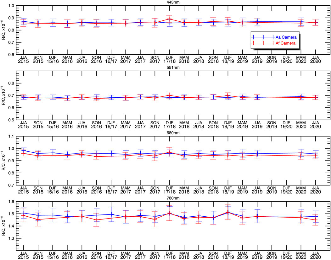
FIGURE 9. Time series of seasonal mean R/C ratios derived from MISR Af (red) and Aa (blue) cameras.
Modeling Earth Polychromatic Imaging Camera Reflectances
EPIC and the LEO instruments view a collocated scene at the same scattering angle in the backscattering region, but may have different viewing and azimuth angles. In this section we conduct a model study to investigate how the differences in viewing geometry affect EPIC calibration coefficients. Such a study is also relevant for the evaluation of the range of any potential systematic differences due to viewing geometry between MODIS Aqua and MODIS Terra, which have different equator crossing times. For this purpose, we calculated reflectance look-up tables (LUT) for water clouds of various brightness. A LUT was calculated for each of the four channels, on a grid of 35 values of cosine of the solar zenith angle (in increments of 0.015), 150 values of cosine of the viewing angle, 181 values of azimuth angle (in increments of 1°), and 19 values of droplet number density, selected to cover the observed range of TOA reflectance. Using the actual geometries of matching EPIC and MODIS scenes, we then calculated what EPIC and MODIS would see, had they flown over such clouds. Specifically, we used the measured MODIS reflectance and viewing geometry (for the actual pixels used for calibration) to look up the cloudy scene that matches the observed MODIS reflectance. Using that scene, we then determined the reflectance that EPIC would measure using its viewing geometry angles for this scene. Thus, we created a set of synthetic (modeled) EPIC reflectances which may be used in place of MODIS reflectances for “calibration.” The procedure is illustrated schematically in Figure 10. The background contour plot shows calculated reflectance field as a function of relative azimuth and view angles for a specific solar zenith angle. Each pair of connected circles and crosses represents MODIS and EPIC positions for a single matching scene. The scenes were randomly selected from the available pool. The calculated reflectance field is selected from the look-up table to match the observed MODIS reflectance for the actual MODIS viewing geometry for each scene. The scene marked by the green line illustrates a situation where MODIS and EPIC would register similar reflectance (same background shade at the ends). For the scene marked by the blue line, EPIC reflectance will be lower than the reflectance registered by MODIS (different background shades at the ends). Repeating this procedure for all available matching scenes allowed us to create a synthetic dataset for this idealized case where both instruments observed scenes of plane-parallel water clouds. If we replace the actual MODIS-observed reflectances with the modeled EPIC ones we can eliminate the influence of the imperfect viewing geometry match between the instruments. In this way we can investigate how calibration gains would change if MODIS were always in the line of sight of EPIC (perfect viewing geometry match). Using only MODIS Terra data, we found the relative differences of mean R/C ratios to be 0.28, 0.1, 0.1, and 0.5% for the 443, 551, 680, and 780 nm channels respectively. For MODIS Aqua the corresponding values were -1.2, −0.02, 0.4, and −2.27%. It can be seen that in this highly idealized case, the average effects of the imperfect viewing geometry match are generally small, except for Aqua in the 780 nm channel. In addition, most of the time, the effects described above influence Aqua and Terra values in opposite directions, so that the results for the combined Aqua + Terra dataset (0.02, 0.09, 0.13, and 0.18% difference, respectively) are very close. It may therefore be advantageous to combine MODIS Terra and MODIS Aqua data for the purpose of EPIC calibration.
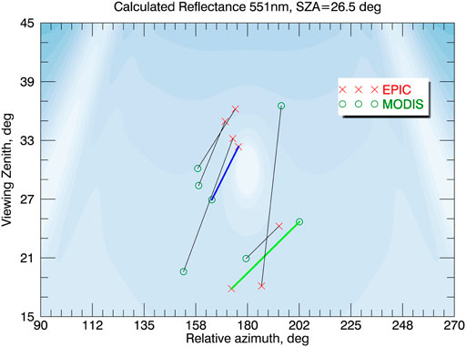
FIGURE 10. A schematic representation of modeling EPIC reflectances. The background contour plot shows calculated reflectance field as a function of relative azimuth and view angles for a specific solar zenith angle. Each pair of connected circles and crosses represents MODIS and EPIC positions for a single matching scene. The scene marked by the green line illustrates a situation where MODIS and EPIC would register similar reflectance (same background shade at the ends). For the scene marked by the blue line EPIC reflectance will be lower than the reflectance registered by MODIS (different background shades at the ends).
We also looked at the ratio of modeled EPIC to measured MODIS reflectance as a function of scattering angle. The results are presented in Figure 11. As can be seen from the figure, in this idealized case, MODIS Terra and Aqua may exhibit biases of up to several percent for the largest scattering angles. This is consistent with measured data in Figure 5, where small increases in the last scattering angle bin may be observed. As can be seen from Figure 10, reflectance gradients are larger in the region close to the exact backscattering. In this region viewing geometry mismatch may result in larger EPIC-LEO reflectance differences. Since the resumption of operations in February 2020, the DSCOVR satellite operates without a gyroscope and relies on its startracker for angular rate information. The satellite is allowed to operate closer to exact backscattering, approaching it every three months to within 2° to conserve fuel for station-keeping. Our results suggest that caution should be exercised when data from such periods are used for calibration purposes. Note however, that, as mentioned above, the biases point in the opposite directions for MODIS Terra and MODIS Aqua and tend to cancel when the data is combined.
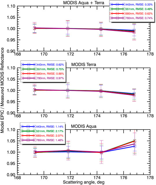
FIGURE 11. Modeled EPIC to measured MODIS reflectance ratios as a function of scattering angle. Top panel: combined Aqua and Terra data, middle panel: MODIS Terra data, lower panel: MODIS Aqua data.
Discussion
We applied the EPIC VIS-NIR calibration algorithm to the full duration of the data record. We assembled database of EPIC-matching data files from MODIS Aqua and Terra, MISR and VIIRS NPP, thus producing uniform EPIC calibration data records against four major LEO radiometers. Calibration gains for data until June 2019 were found to be in excellent agreement with independent published values (Doelling et al., 2019). No significant changes in calibration were observed after the instrument’s exit from safe hold in March 2020. Analysis of seasonal mean R/C ratios revealed that the trends for the full dataset period are not statistically significant except in the 443 nm channel. We conducted an investigation of how DSCOVR’s varying Sun-Earth-Vehicle angle and the distance from Earth could affect the calibration gains. We found that such changes result in less than 1 and 0.5% RMSE variability, respectively. Using MODIS Aqua and MODIS Terra as two independent datasets we analyzed the consistency of the retrieved time series of EPIC calibration gains. Statistical tests indicate that the differences between the two datasets are not significant except in the 780 nm channels, where Aqua-derived coefficients may be around 2% lower compared to Terra-derived ones. Similar consistency analysis was performed using two MISR cameras separately. We found that the gains derived from the forward- and aftward-looking cameras agreed to within 1.5% of each other. These analyses increase our confidence in the robustness of the developed algorithm as applied to multiple LEO radiometers.
Data Availability Statement
Publicly available datasets were analyzed in this study. This data can be found here: DSCOVR EPIC L1B data: https://opendap.larc.nasa.gov/opendap/ MODIS Aqua and Terra L1B data: https://ladsweb.modaps.eosdis.nasa.gov/archive/allData/61/MOD021KM/https://ladsweb.modaps.eosdis.nasa.gov/archive/allData/61/MYD021KM/ MISR L1B data: https://asdc.larc.nasa.gov/data/MISR/MI1B2E.003/ VIIRS L1B data: https://ladsweb.modaps.eosdis.nasa.gov/archive/allData/5000/NPP_VMAES_L1/ MISR Ellipsoid-projected L1B2 data: https://asdc.larc.nasa.gov/MISR/MI1B2E.003 VIIRS L1 data: https://ladsweb.modaps.eosdis.nasa.gov/archive/allData/5000/NPP_VMAES_L1/.
Author Contributions
IG developed the calibration algorithm and performed the data analysis. AM helped in the algorithm development and participated in data analysis. MA provided radiative transfer calculations for the modeling of EPIC reflectances.
Funding
This research was funded by NASA Grant 80NSSC19K0761 “Calibration of the DSCOVR EPIC visible and NIR channels using multiple satellite data.”
Conflict of Interest
The authors declare that the research was conducted in the absence of any commercial or financial relationships that could be construed as a potential conflict of interest.
Acknowledgments
We thank two reviewers and the editor of this paper for their insightful comments, which resulted in a much improved manuscript. The MODIS Terra and Aqua data and VIIRS data were acquired from the Level-1 and Atmosphere Archive and Distribution System (LAADS) Distributed Active Archive Center (DAAC), located in the Goddard Space Flight Center in Greenbelt, Maryland (https://ladsweb.nascom.nasa.gov/). The DSCOVR EPIC and MISR data were obtained from the NASA Langley Research Center Atmospheric Science Data Center.
References
Bruegge, C. J., Chrien, N. L., Ando, R. R., Diner, D. J., Abdou, W. A., Helmlinger, M. C., et al. (2002). Early Validation of the Multi-Angle Imaging SpectroRadiometer (MISR) Radiometric Scale. IEEE Trans. Geosci. Remote Sensing 40, 1477–1492. doi:10.1109/TGRS.2002.801583
Cao, C., De Luccia, F. J., Xiong, X., Wolfe, R., and Weng, F. (2014). Early On-Orbit Performance of the Visible Infrared Imaging Radiometer Suite Onboard the Suomi National Polar-Orbiting Partnership (S-NPP) Satellite. IEEE Trans. Geosci. Remote Sensing 52, 1142–1156. doi:10.1109/TGRS.2013.2247768
Carn, S. A., Clarisse, L., and Prata, A. J. (2016). Multi-decadal Satellite Measurements of Global Volcanic Degassing. J. Volcanology Geothermal Res. 311, 99–134. doi:10.1016/j.jvolgeores.2016.01.002
Carn, S. A., Krotkov, N. A., Fisher, B. L., Li, C., and Prata, A. J. (2018). First Observations of Volcanic Eruption Clouds from the L1 Earth‐Sun Lagrange Point by DSCOVR/EPIC. Geophys. Res. Lett. 45. doi:10.1029/2018GL079808
Channan, S., Collins, K., and Emanuel, W. R. (2014). Global Mosaics of the Standard MODIS Land Cover Type Data. College Park, Maryland, USA: University of Maryland and the Pacific Northwest National Laboratory.
Diner, D. J., Braswell, B. H., Davies, R., Gobron, N., Hu, J., Jin, Y., et al. (2005). The Value of Multiangle Measurements for Retrieving Structurally and Radiatively Consistent Properties of Clouds, Aerosols, and Surfaces. Remote Sensing Environ. 97, 495–518. doi:10.1016/j.rse.2005.06.006
Doelling, D., Haney, C., Bhatt, R., Scarino, B., and Gopalan, A. (2019). The Inter-calibration of the DSCOVR EPIC Imager with Aqua-MODIS and NPP-VIIRS. Remote Sensing 11, 1609. doi:10.3390/rs11131609
Gao, B.-C., Li, R.-R., and Yang, Y. (2019). Remote Sensing of Daytime Water Leaving Reflectances of Oceans and Large Inland Lakes from EPIC Onboard the DSCOVR Spacecraft at Lagrange-1 Point. Sensors 19 (5), 1243. doi:10.3390/s19051243
Geogdzhayev, I. V., and Marshak, A. (2018). Calibration of the DSCOVR EPIC Visible and NIR Channels Using MODIS Terra and Aqua Data and EPIC Lunar Observations. Atmos. Meas. Tech. 11, 359–368. doi:10.5194/amt-11-359-2018
Haney, C., Doelling, D., Minnis, P., Bhatt, R., Scarino, B., and Gopalan, A. (2016). “The calibration of the DSCOVR EPIC multiple visible channel instrument using MODIS and VIIRS as a reference,” in Proc. SPIE 9972, Earth Observing Systems XXI, 99720P, September 19, 2016 (SPIE Optical Engineering + Applications). doi:10.1117/12.2238010
Herman, J., Cede, A., Huang, L., Ziemke, J., Torres, O., Krotkov, N., et al. (2020). Global Distribution and 14-year Changes in Erythemal Irradiance, UV Atmospheric Transmission, and Total Column Ozone For2005-2018 Estimated from OMI and EPIC Observations. Atmos. Chem. Phys. 20, 8351–8380. doi:10.5194/acp-20-8351-2020
Herman, J., Huang, L., McPeters, R., Ziemke, J., Cede, A., and Blank, K. (2018a). Synoptic Ozone, Cloud Reflectivity, and Erythemal Irradiance from Sunrise to sunset for the Whole Earth as Viewed by the DSCOVR Spacecraft from the Earth-Sun Lagrange 1 Orbit. Atmos. Meas. Tech. 11, 177–194. doi:10.5194/amt-11-177-2018
Herman, J., Wen, G., Marshak, A., Blank, K., Huang, L., Cede, A., et al. (2018b). Reduction in 317-780 Nm Radiance Reflected from the Sunlit Earth during the Eclipse of 21 August 2017. Atmos. Meas. Tech. 11, 4373–4388. doi:10.5194/amt-11-4373-2018
JPSS Level 1 Requirements Document (2016). Joint Polar Satellite System (JPSS) Level 1 Requirements Document, JPSS-REQ-1001. https://www.jpss.noaa.gov/assets/pdfs/technical_documents/level_1_requirements.pdf.Final Version: 2.0.
King, M. D., Menzel, W. P., Kaufman, Y. J., Tanré, D., Bo-Cai Gao, B. C., Platnick, S., et al. (2003). Cloud and Aerosol Properties, Precipitable Water, and Profiles of Temperature and Water Vapor from MODIS. IEEE Trans. Geosci. Remote Sensing 41, 442–458. doi:10.1109/tgrs.2002.808226
Kostinski, A., Marshak, A., and Várnai, T. (2021). Deep Space Observations of Terrestrial Glitter. Earth Space Sci. 8, e2020EA001521. doi:10.1029/2020EA001521
Kwiatkowska, E. J., Franz, B. A., Meister, G., McClain, C. R., and Xiong, X. (2008). Cross Calibration of Ocean-Color Bands from Moderate Resolution Imaging Spectroradiometer on Terra Platform. Appl. Opt. 47, 6796–6810. doi:10.1364/ao.47.006796
Lyapustin, A., Wang, Y., Xiong, X., Meister, G., Platnick, S., Levy, R., et al. (2014). Scientific Impact of MODIS C5 Calibration Degradation and C6+ Improvements. Atmos. Meas. Tech. 7, 4353–4365. doi:10.5194/amt-7-4353-2014
Marshak, A., Herman, J., Adam, S., Karin, B., Carn, S., Cede, A., et al. (2018). Earth Observations from DSCOVR EPIC Instrument. Bull. Am. Meteorol. Soc. 99, 1829–1850. doi:10.1175/BAMS-D-17-0223.1
Marshak, A., and Knyazikhin, Y. (2017). The Spectral Invariant Approximation within Canopy Radiative Transfer to Support the Use of the EPIC/DSCOVR Oxygen B-Band for Monitoring Vegetation. J. Quant. Spectrosc. Radiat. Trans. 191, 5197–5202. doi:10.1016/j.jqsrt.2017.01.015
Marshak, A., Várnai, T., and Kostinski, A. (2017). Terrestrial Glint Seen from Deep Space: Oriented Ice Crystals Detected from the Lagrangian point. Geophys. Res. Lett. 44. doi:10.1002/2017GL073248
MODIS Characterization Support Team (2006). MODIS Level 1B Product User’s Guide. https://mcst.gsfc.nasa.gov/sites/mcst.gsfc/files/file_attachments/M1054.pdf.
Scarino, B. R., Doelling, D. R., Minnis, P., Gopalan, A., Chee, T., Bhatt, R., et al. (2016). A Web-Based Tool for Calculating Spectral Band Difference Adjustment Factors Derived from SCIAMACHY Hyperspectral Data. IEEE Trans. Geosci. Remote Sensing 54 (5), 2529–2542. doi:10.1109/tgrs.2015.2502904
Toller, G., Xiong, X., Sun, J., Wenny, B. N., Geng, X., Kuyper, J., et al. (2013). James Kuyper, Amit Angal, Hongda Chen, Sriharsha Madhavan, Aisheng Wu,Terra and Aqua Moderate-Resolution Imaging Spectroradiometer Collection 6 Level 1B Algorithm. J. Appl. Remote Sens 7 (1), 073557. doi:10.1117/1.JRS.7.073557
Varnai, T., Marshak, A., and Kostinski, A. B. (2020). Deep Space Observations of Cloud Glints: Spectral and Seasonal Dependence. IEEE Geoscience and Remote Sensing Letters, 1–5. doi:10.1109/LGRS.2020.3040144
Yang, B., Knyazikhin, Y., Mõttus, M., Rautiainen, M., Stenberg, P., Yan, L., et al. (2017). Estimation of Leaf Area index and its Sunlit Portion from DSCOVR EPIC Data: Theoretical Basis. Remote Sensing Environ. 198, 69–84. doi:10.1016/j.rse.2017.05.033
Yang, Y., Marshak, A., Mao, J., Lyapustin, A., and Herman, J. (2013). A Method of Retrieving Cloud Top Height and Cloud Geometrical Thickness with Oxygen A and B Bands for the Deep Space Climate Observatory (DSCOVR) Mission: Radiative Transfer Simulations. J. Quantitative Spectrosc. Radiative Transfer 122, 141–149. doi:10.1016/j.jqsrt.2012.09.017
Yang, Y., Meyer, K., Wind, G., Zhou, Y., Marshak, A., Platnick, S., et al. (2019). Cloud Products from the Earth Polychromatic Imaging Camera (EPIC): Algorithms and Initial Evaluation. Atmos. Meas. Tech. 12, 2019–2031. doi:10.5194/amt-12-2019-2019
Keywords: deep space climate observatory/earth polychromatic imaging camera, calibration, moderate resolution imaging spectroradiometer, multi-angle imaging spectroradiometer, visible infrared imaging radiometer
Citation: Geogdzhayev IV, Marshak A and Alexandrov M (2021) Calibration of the DSCOVR EPIC Visible and NIR Channels using Multiple LEO Radiometers. Front. Remote Sens. 2:671933. doi: 10.3389/frsen.2021.671933
Received: 24 February 2021; Accepted: 10 May 2021;
Published: 21 May 2021.
Edited by:
Oleg Dubovik, CNRS, UMR8518 Laboratoire d’optique atmosphèrique (LOA), FranceReviewed by:
Jeffrey Czapla-Myers, University of Arizona, United StatesDavid Doelling, National Aeronautics and Space Administration (NASA), United States
Copyright © 2021 Geogdzhayev, Marshak and Alexandrov. This is an open-access article distributed under the terms of the Creative Commons Attribution License (CC BY). The use, distribution or reproduction in other forums is permitted, provided the original author(s) and the copyright owner(s) are credited and that the original publication in this journal is cited, in accordance with accepted academic practice. No use, distribution or reproduction is permitted which does not comply with these terms.
*Correspondence: Igor Geogdzhayev, aWdvci52Lmdlb2dkemhheWV2QG5hc2EuZ292