Explicit mathematical models of multiple polarization-measurements and the Einstein-Bohr debate

We present mathematical models that also may be formulated as computer models for experiments that feature single photon resolution and multiple pairs of polarizers to determine the sorting into ordinary and extraordinary channels. The models are based on Einstein’s hypothesis of elements of physical reality that determine the photon properties and are at first developed for Malus-type experiments. It is then shown that analogous models apply to the well-known Clauser-Aspect-Zeilinger experiments and violate all Bell-type inequalities without violating Einstein’s separation principle. The Bell-type inequalities do not apply to the actual experiments, because they cannot obey the physically necessary symmetry with respect to polarizer-pair rotations. We believe that these findings suggest a change of current interpretations of quantum entanglement away from instantaneous influences at a distance, as promoted in the physics Nobel-lectures 2022, and back toward Einstein’s ideas as well as the more recent ideas of Gerard ‘t Hooft.

1 Introduction

The well-known debate between Einstein and Bohr can be summarized by the slogan “relativity versus probability”. Bohr maintained that, with respect to quanta, probability was a fundamental feature of nature and Pauli explained that in contrast to Bohr “… Einstein … considered quantum mechanics to be something like statistical gas theory … ” Einstein resisted indeed the Born-type probability theories that are defined without the involvement of elements of physical reality. At first glance, the differences of the two views appear minor. Probability theorists assume that Tyche, the goddess of fortune choses elements $\omega$ of the sample space $\mathrm{\Omega }$ and a particular ${\omega }_{act}$ that determines the outcome of the measurement of the moment. Einstein in essence insists that in physical experiments we need to deal with physical properties $\lambda \in \mathrm{\Lambda }$ and with corresponding ${\lambda }_{act}$ that provide the related ${\omega }_{act}$ with a physical meaning. However, Bohr and his school pointed to the fact that the possible physical properties of quanta that determine the actual events, such as the complementary values of location and velocity, cannot even exist before the moment of measurement, owing to the Uncertainty Principle.

It took Einstein years to produce an incisive response to Bohr and the teachings of the Copenhagen school. With Podolsky and Rosen he formulated a manuscript (now called the EPR paper (Einstein et al., 1935)) that offered a possibility to determine complementary properties of the quanta as follows: create pairs of quanta that are correlated by physical law. Then, if you measure the velocity of one piece of the pair you may deduce the velocity of the other from the physical law. Measuring the position of the other piece gives you, therefore, both properties. The Uncertainty Principle is not violated, because only one measurement is performed on each quantum, to obtain both complementary properties. We may, thus, believe that Tyche’s choices also represent elements of physical reality.

The actually performed first direct experiments related to EPR were a variation of a suggestion of Bohm: Kocher and Commins (Kocher and Commins, 1967) used measurements involving photon pairs and the concept of polarization. Judging from their results, Einstein’s ideas appeared to be possible. Kocher and Commins found excellent experimental correlations (entanglement) for equal polarizer angles that could be seen as representing a law of nature for the photon-pairs and the corresponding existence of properties.

However, the well-known inequality of J. S. Bell (Bell, 1964) has led to a different explanation of the photon-pair experiments. Note that Bell’s original theory was describing spin $\frac{1}{2}$ quantum entities and Stern-Gerlach measurements. His work and its important logical implications concerning such experiments, may be “translated” for photon (spin 1) related experiments by simply including a factor of two in the pertinent equations, which we have done below. We may then imagine that Bell’s work has considered experimental sequences, each having different polarizer directions and maintained that the average measurement outcomes must fulfill an inequality. Strangely enough, this inequality was not obeyed by the results of quantum mechanics. It also was convincingly shown by numerous groups related to the 2022 Nobel Laureates Clauser, Aspect and Zeilinger that the actual experiments also contradicted the inequality of Bell and a similar inequality derived by Clauser, Horn Shimony and Holt (CHSH) (Clauser et al., 1969). We assume at this point that the reader is familiar with Bell-CHSH-type inequalities. We will, however, include below a fairly detailed description of the CHSH inequality and its derivations.

The crucial question is why Bell’s model does not agree with quantum theory. Bell had an answer to this question. He was convinced that he, CHSH and others had derived the inequalities more or less exclusively based on Einstein’s physics and in particular Einstein’s separation principle and corresponding “local” properties of physical events (following from the limitations of all velocities to a maximum of the speed of light in vacuum). The violation of their inequalities indicated to Bell and CHSH that a special interpretation of the photon correlation (entanglement) that included “non-local” effects must be in order. As we will show, it is important to distinguish between different forms of “non-localities”, in order to understand what indeed the Bell-CHSH inequalities mean. The form that Einstein objected to was any instantaneous influences at a distance, such as a measurement in Tokyo influencing instantly the outcome of a measurement in New York. In contrast to this particular non-locality that Einstein called “spooky”, there are physically natural (at least to Einstein) non-localities. For example, any properly relativistic model requires the theoretician’s consideration of physical events relative to each other and involves, if these events are spatially separated, non-local theoretical considerations to start with. Such a non-locality may, however, retrospectively be explained without instantaneous influences by use of a space-time system. It is important to distinguish between the permitted global thinking of a theoretician using a space-time system and inappropriate introductions of instantaneous non-local occurrences. These subtle problems related to the physical nature of non-localities are enhanced by the mathematical complications of set theoretic probability that must be the basis of the derivation of the Bell-CHSH inequalities.

We highlight these problems and questions by detailed mathematical- and computer-models for two types of experiments: the Malus-type as explained in the Feynman lectures (Feynman Lectures, 1965) and the EPRB-type, including the experiments of Kocher and Commins (Kocher and Commins, 1967), of Aspect and coworkers (Aspect, 2015) and of Kwiat (Kwiat et al., 1999) and coworkers. Before doing so, however, we discuss what we mean by words like “local” or “measurement” etc. and how to avoid prejudicial conclusions about them.

2 Definitions and prejudices in discussions related to the Bell-CHSH inequalities

Concepts often involved when discussing Bell-CHSH, are those of entanglement, measurement, experiment, local vs. non-local, as well as deterministic vs. probabilistic. We also use these terms but only subject to the following considerations:

It is commonly claimed and believed that the Bell-CHSH inequalities must be valid within Einstein’s framework and definitions of physical principles. We put our main emphasis on the refutation of this important point and, therefore, do not involve concepts of quantum mechanics other than those pioneered by Einstein.

As a consequence, we never use any contemporary quantum mechanical meaning of the word “measurement”. What we mean by measurement follows from the most elementary explanations such as “a detector clicks”, or in another situation “a detector clicks after a photon has passed a polarizer”. We agree with the standard definition found on Internet-dictionaries: “Measurement is the quantification of attributes for an object or event, which can be used to compare with other objects and events.” It nicely encompasses the importance of the relative comparison of attributes and events. With the expression “experiment” we also refer to the dictionary meaning of “a scientific procedure undertaken to make a discovery, test a hypothesis, or demonstrate a known fact”.

When we talk about entanglement, we do mean something related to the quantum-entanglement as defined already by Schrödinger. In our present utilization of the word, we only refer to some basic correlation and hope that a future more detailed interpretation will benefit from our contributions to an understanding of the work of Bell-CHSH.

The concepts of “local” and “deterministic” appear in a vast Bell-CHSH-related literature, often with different meaning. We believe that what is acceptable as “local theory” spans a wide range that is not necessarily accepted by the followers of Bell-CHSH. For example, Einstein’s relativity teaches about measurement outcomes relative to each other. If these outcomes have a space-like distance, then naturally any relativistic thought-process of a theoretician involves non-local factors, as already mentioned. Yet, there are not many physicists who would think of such relativistic thinking as something that is physically undesirable or even forbidden. We, therefore, have limited ourselves to talk about “local” and “non-local” only in connection with specific experiments and measurements that we model also by computers to illustrate the non-local thought processes versus the local causal machinery that mother nature uses (according to Einstein) in a given measurement station.

We dismiss out of hand all definitions of “local” and “deterministic” that use certain conditional probabilities: Bell and followers have frequently used probabilities conditional to one particular element of physical reality (Gisin, 2012). Because the elements of physical reality may involve continua (distances, times, etc.), the Lebesgue measure of the probability that such a particular element of physical reality is actually encountered may be zero. Consequently, such a conditional probability cannot sensibly be defined within the confines of set theory (for additional explanations and problems see (Hess, 2023)).

Regarding the concepts of “deterministic vs. probabilistic”, we also adhere to the common-sense definition that: “Deterministic models produce the same exact outcome for any given exact same set of inputs, while probabilistic models do not.” However, we have to be cautious with this definition in the following respect. Bell’s model contains the symbols of Einstein’s elements of physical reality that may be randomly selected out of a continuum and may be modeled, as we will do below, by random real numbers out of the interval [-1, +1]. The subtle point is now that one may not be permitted to use the same real number again for different model-events. While it may be true then that we have the same exact outcome for the same exact input, the probability to encounter the same exact input may be zero. Such a model is, therefore, comparable to models of radioactive decay and must be seen as probabilistic. The consequences of this fact for the interpretation of experiments related to Bell-CHSH were discussed in (Jakumeit and Hess, 2024). Bell’s model is, therefore, probabilistic depending on the nature of his variable $\lambda$, particularly whenever $\lambda$ is used just like the general $\omega$ of probability theory (as used by many researchers).

We like furthermore to point to the fallacies of the very common Alice and Bob reasoning regarding locality considerations. Alice controls one polarizer angle without knowing anything about Bob, who controls the other polarizer angle. The confusion of the Alice-Bob stories arises from the fact that Alice and Bob are seen as somehow representing mother nature, who must, according to Einstein’s views, indeed be local causal. That does not mean however that a theoretician, say Charly, does not know global macroscopic instrument arrangements and designs the local causation of his model by using his global knowledge and the space-time system. For the particular case of EPRB experiments, Charly must know about the ancient principle that events may only be evaluated relative to each other, which Alice and Bob cannot accomplish to start with, because they do not know about each other. Without global physical laws and a space-time system, even the correlation of clocks in distant cities becomes a mystery.

We ask the reader not to abandon our reasoning, because of prejudices regarding the use and meaning of the discussed important terms.

We also like to point toward other important criticisms involving views more or less different to ours presented here. In particular, the concept of “contextuality” has been used in a number of ways to discuss violations of the Bell-CHSH inequalities. We do not use the loaded word “contextual” at all but only talk about “events being evaluated relative to each other”. Of course, in the case of spatially distant experiments relative evaluation encompasses a lot of the meaning of “contextuality”. Numerous important works have discussed related violations of Bell-CHSH. Particularly relevant points have been presented in the works of Khrennikov (2009) (see also the well-known Växjö conferences) and Kupczynski (2020) as well as references in their works.

3 Malus-type experiments for single photons with sequential polarizers

3.1 Geometry and measurement-outcomes of the Malus-type experiments

Perhaps the most illuminating experiment, at least with respect to modeling and the Alice-Bob “locality” assumptions by Bell and followers, is the standard Malus-type experiment performed with single photon resolution. Consider two special polarizers, Wollaston prisms, in sequence to the right of a single-photon source $S$ (Wollaston prisms permit a clearer formulation of the arguments, although they have not necessarily been used in all actual experiments). The photons propagate in $z$- direction and are sorted by the Wollaston prisms into two sets one named ordinary ${\mathrm{\Lambda }}_o$ and the other extraordinary ${\mathrm{\Lambda }}_e$. The properties of these sets depend, in general, on the geometric configuration of the Wollaston prisms. We characterize this configuration throughout this paper by an angle in the $x,y$ plane denoted by the variable $j=a,a^{\prime },\dots$ for the primary Wollaston $W_1$ and by $j^{\prime }=b,b^{\prime },\dots$ for any secondary Wollaston $W_2$.

Assume now that the source $S$ emanates $N$ photons that behave in the following way. Passing $W_1$ with a given configuration angle, for example, $j=a$, leads to the sorting of about $\frac{N}{2}$ photons into the ordinary set that we denote now by ${\mathrm{\Lambda }}_o^a$ and about $\frac{N}{2}$ photons into the extraordinary ${\mathrm{\Lambda }}_e^a$ . We cannot deduce from such measurements more than the fact that Wollaston prisms, no matter how configured, lead to binary sorting that may be influenced by the given polarizer direction (angle). This angle is just defined within our rather arbitrary global coordinate system and, therefore, single photon measurements performed with a single polarizer, have only limited significance for distant correlations.

Sequential measurements with two additional Wollaston prisms $W_2$ and $W_2^{*}$ (called analyzers), do give us more interesting information. $W_2$ is arranged to pick up the ordinary channel of $W_1$ and deals, thus, with the set ${\mathrm{\Lambda }}_o^j$, while $W_2^{*}$ deals with the extraordinary channel of $W_1$ and the set ${\mathrm{\Lambda }}_e^j$. We have illustrated the geometry of the Wollaston prisms including the source $S$ in Figure 1. Note that one cannot have both $W_2$ and $W_2^{*}$ precisely perpendicular to the z-axis with their face in the x-y plane, but it is well known how to experimentally approximate this situation and we just assume for the mathematical model that all Wollaston prisms are perpendicular to the z-axis, which is the direction of the photon propagation. The Wollaston’s rotation-angle is in the x-y plane starting with zero in the x-direction.

Figure 1

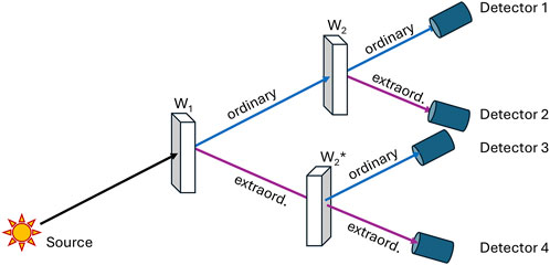
Figure 1. Experimental arrangement for single-photon Malus-type experiments. The polarizer is represented by Wollaston prism $W_1$ and the analyzers by $W_2$ and $W_2^{*}$, respectively.

The two sets ${\mathrm{\Lambda }}_o^j$ and ${\mathrm{\Lambda }}_e^j$ are now analyzed by Wollaston prisms $W_2$ and $W_2^{*}$ that sort these sets into the sets ${\mathrm{\Lambda }}_o^{j,j^{\prime }}$, ${\mathrm{\Lambda }}_e^{j,j^{\prime }}$ and ${\mathrm{\Lambda }}_o^{*j,j^{\prime }}$, ${\mathrm{\Lambda }}_e^{*j,j^{\prime }}$, respectively.

Einstein’s hypothesis is that the photons of these sets have certain properties. We denote these properties of the photons that are contained in the various sets above by the lower-case symbols: ${\lambda }_o^{j,j^{\prime }}$, ${\lambda }_e^{j,j^{\prime }}$, ${{\lambda }^{*}}_o^{j,j^{\prime }}$ and ${{\lambda }^{*}}_e^{j,j^{\prime }}$ and take them as the basis for our Einstein-type model. This second (relative) sorting follows a law of nature, known for very large numbers $\frac{N}{2}$ of photons as the law of Malus and states:

Of all the photons that transfer into the ordinary channel of $W_1$, an approximate number of

$\frac{N}{2}{\cos }^2\left(j-j^{\prime }\right)$

photons will transfer into the ordinary channel of $W_2$ for large $N$. The numbers found in the extraordinary channel of $W_2^{*}$ follow the same law. As is evident, this law is invariant to rotations of the coordinate system as well as the rotation of the Wollaston prisms around the z-axis. Therefore, we may choose $j=0$, without restriction of generality, put $j-j^{\prime }=\theta$ and obtain in this way the Malus law in its usual notation:

$\frac{N}{2}{\cos }^2\left(\theta \right)$

The connection of the corresponding expressions in terms of the energy of macroscopic electromagnetic fields (instead of large numbers of photons), has been described in detail in introductory texts and also has been shown to be fully consistent with the laws of quantum mechanics (Feynman Lectures, 1965; Baym, 1973).

In order to provide an Einstein type model for the single photon Malus law we need to develop a model that is in principle described by a set theoretic probability theory that features events ${\omega }_{act}$ that also have a meaning as Einstein’s elements of physical reality ${\lambda }_{act}$. We further need to link this element of physical reality to the measurement outcomes for the events of the photons interacting with the Wollaston prisms. This link may be achieved as follows.

3.2 Set theoretic mathematical model for the Malus-type experiments

It has been shown in great detail by David Williams in his textbook on probability theory (Williams, 2001) that experiments describing the possible machineries of our surrounding macroscopic world by using probabilities may be modeled by the set theoretically precise Fundamental Model of Probability Theory. The patient reader must remember that set-theoretic mathematics deals with a “fundamental triple” that includes a sample space $\mathrm{\Omega }$, a sigma algebra of subsets of $\mathrm{\Omega }$ and a unique probability measure P.

The Fundamental Model of probability theory uses the interval $\left[0,+1\right]$ of the real numbers for $\mathrm{\Omega }$. Every event of actual measurements may be simulated by a real number out of this interval. The events are, as usual, denoted by $\omega \in \mathrm{\Omega }$. As mentioned, Tyche, the goddess of fortune, picks one such $\omega$ denoted by ${\omega }_{act}$ to instigate a certain actual event. For ${\omega }_{act}$ drawn uniformly from the interval [0,1] the probability that ${\omega }_{act}$ lies in a sub-interval $\left[0,x\right]$ is given by $x$ (Williams, 2001).

To simulate the actual polarizer experiments by involving real numbers for the photon properties, it is convenient (as we will see below) to generalize the Fundamental model to include the extended interval $\left[-1,+1\right]$ instead of $\left[0,+1\right]$, which is straightforward. We introduce now the notation and conventions similar to Bell and denote the measurement outcomes by two-valued functions, $A$ for polarizer $W_1$ and $B$ for polarizers $W_2$ as well as $W_2^{*}$. We define $A=B=+1$ if the photon is found always in the ordinary channel and $A=B=-1$, if it is always found in the extraordinary channel. Our main postulate is that one can indeed model the photon properties for the particular experiment in question by the real numbers of the Fundamental model. The possibility of mapping the elements of physical reality onto the real interval $\left[-1,+1\right]$ is indeed a plausible assumption, because we consider only relative outcomes. For a given polarizer angle $j$, we may then sort the outcomes of $A$ into two sets that depend only on the sign of the number that models the properties of the photon, because we know that the polarizer accomplishes just such sorting, hereby connecting these sets to the polarizer direction within our arbitrarily chosen coordinate system.

The sorting of the analyzers $W_2$ and $W_2^{*}$ into ordinary and extraordinary sets can then be further modeled as follows: the photon stays with the same sorting that $W_1$ has accomplished (extraordinary or ordinary), meaning $B=A$ if and only if:

$\left|{\lambda }_{e,o}^j\right|\le {\cos }^2\left(\theta \right).(1)$

According to the Fundamental Model, the probability measure that we indeed encounter such $\left|{\lambda }_{e,o}^j\right|$ equals precisely ${\cos }^2\left(\theta \right)$, which leads to the law of Malus-type for large $N$. The absolute value is now used because we have extended the Fundamental interval to $\left[-1,+1\right]$.

Notice that the use of the relative polarizer angles $\theta$ in Equation 1 appears completely natural, because the photon has passed both polarizers and may be sorted into the appropriate sets due to its properties that are recognized by both polarizers. No “forbidden” non-locality has ever been attributed to the use of $\left(j^{\prime }-j=\theta \right)$ for that particular experiment in contrast to the EPRB-type experiments. We note in passing that mathematically there exists almost no difference between this Malus-type experiment and the EPRB-type as soon as Einstein’s hypothesis of elements of physical reality is made. One of the reasons for this fact is that we do not need to assume that the Wollaston polarizers change the properties of the photons. It is sufficient to assume that the photon properties are recognized by the polarizers and used for the sorting. In this connection it is important to realize the difference between the properties described by $\lambda$ immediately after the emission of the photons and the properties (actual or model) that mark the photons and $\lambda$ after passing the polarizers. It is these properties that may be represented by markers related to the law of nature that determines the outcomes. We will return to this important point below.

4 Polarizers on opposite sides of a source

We now turn to the configuration with the polarizers on opposite sides of the source as illustrated in Figure 2, which shows the experimental arrangement along the lines of the EPR ideas with the modifications by Bohm and first implementation using photon-pairs and a stretched film of poly-vinyl alcohol containing oriented anisotropic molecules instead of a Wollaston prism, by Kocher and Commins (Kocher and Commins, 1967).

Figure 2

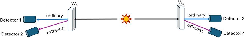
Figure 2. Experimental arrangement for entangled-photon for EPRB-Kocher-Commins-type experiments.

Unlike the Malus-type single-photon experiment, this experiment has been performed by many researchers starting with Kocher and Commins and continuing with significant extensions by groups around Clauser et al. (1969), Aspect (2015), Giustina et al. (2015), Kwiat et al. (1999) and others.

We use the same notation that we have used in the previous section, in order to highlight the important similarities and differences with respect to the modeling of the Malus-type. Wollaston $W_1$ is now arranged to the left of the source $S$ and Wollaston $W_2$ to the right as shown in Figure 2. Wollaston $W_2^{*}$ is being merged with $W_2$.

The source emanates now correlated photon-pairs (see explanations by Kocher and Commins (1967)). We assume in the following theoretical discussions that the correlation of the photon-pair is ideal and such that each photon is being recognized according to its properties in identical fashion by $W_1$ and $W_2$. In other words, the photons are identical twins as viewed with $W_1$ or $W_2$.

As for the case of the Malus-type experiments, we need to maintain the principle that the measurements of events have only physical meaning relative to each other. Alice and Bob, knowing nothing about each other, may only judge their local measurements relative to their own previous measurements and thus conclude that the clicks of their detectors are random, corresponding to the detections for ordinary and extraordinary channels of $W_1$ and $W_2$, respectively. If we wish to probe into the distant relative measurement-outcomes, we need to employ a theoretician, Charly, who must involve global factors into his thinking, while still admitting only local causes for the interactions and measurement-outcomes on a given side. As Einstein told Heisenberg: “it is the theory that determines what we can measure” and it is historically true that great experimentalists have also had a deep grasp of theory and vice versa.

Therefore, if we wish to proceed to the understanding of the non-local distant correlations, we need to clearly distinguish on one hand between the theoretical knowledge that Charly must have about the global situation and on the other hand the local causality that must apply according to Einstein for the events in the respective stations.

The natural local interactions involve the polarizer angles $j$ and $j^{\prime }$ at the time of interaction, which is measured by local synchronized clocks. Charly describes the local configurations by use of his global coordinate system. Therefore, the local configurations of the polarizers at the time $t_n^1$ for polarizer $W_1$ and $t_n^2$ for polarizer $W_2$ may both assumed to be available to Charly within the space-time system, while Nature has available just the single local configurations. Charly, of course, can only find out later what the actual polarizer configurations were, by checking the records of measurement at the registered clock-times.

Note, that the experimenters must, as Charly does, involve more than their local knowledge of equipment configurations if they wish to consider relative outcomes. They too must have a global coordinate system and synchronized clocks (a space-time system), whenever they attempt to compare the outcomes $A,B$ and determine whether $A=B$ (Aspect, 2015). They also have worked with fixed polarizers and without clocks during the whole sequence of measurements (see, for example, some of the measurements in (Kwiat et al., 1999)).

What is it then that can be measured, while the global rules of relative evaluation as well as the rules of local causes are strictly obeyed? Consider the case of registered detector clicks $A=\pm 1$ and $B=\pm 1$. Relatively speaking, we have then four possibilities of interesting physical outcomes and we collapse them by symmetry onto two: we either have $A=B$ or $A\ne B$. All relative physics must, therefore, be contained in the numbers of equal versus not-equal outcomes of the experimental runs. Importantly, it turns out that the results of $A=B$ vs $A\ne B$ are also the only results used to obtain the Bell-CHSH inequalities. Charly needs to model, therefore, only the number $N_{eq}$ of equal outcomes $A=B$ that contains all interesting physics. The number of not equal outcomes $N_{neq}$ is given by $N_{neq}=N-N_{eq}$. Thus, Charly is not interested in modeling natures outcomes for $A$ and $B$ separately but is satisfied to obtain a correct model for the product $A·B$, which also happens to be all that Bell-CHSH have needed and used in their work.

We now apply the methods that we have developed for the Malus-type experiment in the previous section: $W_1$ is thought to establish the connection of the actual experiment to the global coordinate system and sorts the incoming photon of the pair into two sets, while $W_2$ analyzes the incoming twin-photon corresponding to its properties and “markers” that are for all practical purposes assumed identical for the twins. Because we treat $W_2$ as the analyzer we have a situation which is completely analogous to the Malus-type experiments. To see this fact, imagine the measurement of the $W_1$ detector to be performed slightly earlier, exactly as it is for the Malus type measurements. This analogy permits us to sorting the identical twins as we did in the Malus-type experiments and as is described next. Of course, we may also exchange the roles of $W_1$ and $W_2$. Imagining that the measurement involving $W_1$ happens before that involving $W_2$, is only used to illustrate the analogy to the Malus type experiment.

There exists one big difference of the EPRB-type experiments to the Malus-type. For these latter, we could use $W_2$ and $W_2^{*}$ to further process the ordinary and extraordinary channels. Without this possibility we must employ very careful procedures that avoid the introduction and appearance of instantaneous distant influences.

We still use Einstein’s elements of physical reality that may be imagined as “markers” of the single photons that are the causes for $W_1$ to guide the incoming photon of the pair toward the $+1$ or the $-1$ detector and thus makes it a member of the sets ${\mathrm{\Lambda }}_o^j$ or ${\mathrm{\Lambda }}_e^j$, respectively, after being detected. Note that we must postulate that these sets depend on the angle $j$, because otherwise the polarizer-geometry would have no influence. We have denoted their elements by ${\lambda }_o^j$ or ${\lambda }_e^j$ for the Malus-type experiments, but add now an index $n$ for the measurement number in order to obtain the notation of ${\lambda }_{on}^j$ or ${\lambda }_{en}^j$, respectively.

In our opinion, this approach synthesizes the views of Einstein and Bohr. The properties of the photons and photon pairs are only known after at least one measurement (with say $\mathrm{j}=\mathrm{a}$) was performed, relative to which other measurements are evaluated and analyzed.

We turn now to our model in which all of Einstein’s elements of physical reality are simulated by real numbers out of [-1, +1]. Each of the randomly selected numbers signifies different properties and is denoted by ${\lambda }_n$ with $n=1,2,3,\dots ,N$. We postulate further that there exists a one-to-one correspondence of the Einsteinian elements (that occur in the actual measurements for a given polarizer angle, e.g., $j=a$) and our model-numbers ${\lambda }_n$. Each ${\lambda }_n$ is, therefore being mapped to represent one of the specific elements ${\lambda }_{on}^j$ or ${\lambda }_{en}^j$ arising from the measurements involving $W_1$ and belonging to the sets ${\mathrm{\Lambda }}_o^j$ or ${\mathrm{\Lambda }}_e^j$ for the selected value $j=a$. The source has sent a twin element toward the analyzer $W_2$, and that analyzer is being represented by the function $B\left(j^{\prime }=b,{\lambda }_n={\lambda }_{on}^{j=a}\right)$. The evaluation of that function may, thus, depend on both $j=a$ and $j^{\prime }=b$, because both angles appear in the entirely local domain of the function $B$. The concrete form of the function is not known for certain and may not even exist. Nevertheless, Charly may guess the value of $j$ and base his model on this guess, while validating the model later on when the information about the value of $j$ is available to him (as in the model of (Jakumeit and Hess, 2024)).

Based on all these facts, Charly lets:

$A\left(j,{\lambda }_n\right)=sign\left({\lambda }_n\right)(\mathrm{2a})$

and

$B\left(j^{\prime },{\lambda }_n\right)=sign\left({\lambda }_n\right)\text{\hspace{0.17em}if\hspace{0.17em}and\hspace{0.17em}only\hspace{0.17em}if\hspace{0.17em}}\left|{\lambda }_n\left|\le \right.{\cos }^2\left(j^{\prime }-j\right)\right.$

in order to model the law of nature that determines the equal and not-equal relative outcomes $\left(A=B\right)$.

We do admit that our multiple assumptions, although very plausible, do not let us prove with certainty that quantum-non-localities are not involved in any way. Such proof can probably never be achieved. One simply cannot prove that “spooky” influences (in Einstein’s sense) do not exist.

There is just one minor modification necessary in order to fully compare this model with the experiments of Kocher, Clauser, Aspect and others. All these well-known actual experiments use complete anti-correlation instead of correlation. To obtain the results for anti-correlation, we just need to put

$B{j}^{\prime },{\lambda }_n=sign\left({\lambda }_n\right)(\mathrm{2b})$

If and only if:

$\left|{\lambda }_n\left|>co\right.s^2\left(j^{\prime }-j\right).\right.(\mathrm{2c})$

Equations 2a-c permit us to derive the well-known measured averages by our model. For any given polarizer-angle pair $\left(j,j^{\prime }\right)$, we denote the normalized sum of $N$ measurements by $D\left(j,j^{\prime }\right)$ $:$

$D\left(j,j^{\prime }\right)=\frac{1}{N}{\displaystyle \sum _{n=1}^N}A\left(j,{\lambda }_n\right)B\left(j^{\prime },{\lambda }_n\right)(3)$

In the limit of $N\to \infty$, we obtain from expressions (Equations 2a-c) of our model:

$D\left(j,j^{\prime }\right)=-\cos \left(2\left(j^{\prime }-j\right)\right)(4)$

This latter result agrees with the results of quantum mechanics, which appears entirely natural, because it represents in essence a Malus-type law and is very closely connected to the measurement-outcomes for single photon Malus type experiments.

This very result is, however, incompatible with the Bell-CHSH inequalities derived in (Clauser et al., 1969). How can that be? The obvious reason is that Bell-CHSH and followers have used the same measurement number $n$ for different polarizer setting pairs. As long as one considers only one polarizer-angle pair (no matter which), this is correct. However, as soon as one calculates the four sums $D\left(j,j^{\prime }\right)$ that are the basis for the Bell-CHSH inequality, one needs to realize that different polarizer-angle pairs must have, in general, a different measurement number. As we show next, this lack of precise mathematical labeling still permits the correct derivation of the Bell-CHSH-type inequalities if (and only if) Einstein’s elements of physical reality are countable (see also (Jakumeit and Hess, 2024)). However, just in this very case of countability, the so derived Bell-CHSH inequalities are not invariant under rotations of the polarizers around the z-axis and, therefore, physically speaking, unacceptable

5 Bell-type inequalities as derived in the terms of the Fundamental Model

Bell-CHSH deduced by elementary manipulations that one expects:

$CHSH=:\left|D\right.\left(a,b\right)-D\left(a,b^{\prime }\right)+D\left(a^{\prime },b\right)+D\left(a^{\prime },b^{\prime }\right)\left|\le 2\right.(5)$

Key to this finding is that they used identical ${\lambda }_n$ in all the sums of Equation 3 for all values of $\left(j,j^{\prime }\right)$, meaning for $\left(a,b\right),\left(a,b^{\prime }\right),\left(a^{\prime },b\right)$ and $\left(a^{\prime },b^{\prime }\right)$.

Notice that identical ${\lambda }_n$ permit the derivation of Equation 5 from Equation 3, because then all $4N$ measurement-outcomes may be described by N quadruples of the form:

$A\left(a,{\lambda }_n\right)·B\left(b,{\lambda }_n\right)-A\left(a,{\lambda }_n\right)·B\left(b^{\prime },{\lambda }_n\right)+A\left(a^{\prime },{\lambda }_n\right)·B\left(b,{\lambda }_n\right)+A\left(a^{\prime },{\lambda }_n\right)·B\left(b^{\prime },{\lambda }_n\right)(6)$

which are now each cyclically connected (with three products known, the fourth is fully determined) and, therefore, all quadruples are equal to $+2$ or $-2$. However, for our Fundamental model, the ${\lambda }_n$ are represented by real numbers chosen randomly out of $\left[-1,+1\right]$. The probability to obtain the same ${\lambda }_n$ for any different model-measurement is zero and this applies also to any actual measurement if Einstein’s elements of physical reality indeed correspond to a continuum that can be mapped onto (or modeled by) the interval [-1, +1] of real numbers.

As mentioned, Bell-CHSH have deduced their use of the identical ${\lambda }_n$ in each of the four sums from the fact that the emitted elements of physical reality may not depend on the polarizer angles, because these may be chosen in the last moment just before the actual measurement and indeed have been so chosen in all Aspect-type (Aspect, 2015) experiments. As mentioned, however, that fact does not mean that the ${\lambda }_n$ of Equation 6 must be identical for all polarizer angle pairs. In strict mathematical terms, the ${\lambda }_n$ are only identical in approximately all quadruples if their number $M$ is countable (finite) and if the number of measurements $N\gg M$. (We do not include the case of countable infinite into our discussions in spite of the fact that similar situations can be constructed with countable infinite sets such as rational numbers.)

The astounding conundrum of the Bell-CHSH inequalities arose from the conviction of Bell and followers that their derivations followed mostly from Einstein’s separation principle. They did not realize that their derivation required additional mathematical conditions regarding the cardinality of Einstein’s elements of physical reality and a certain cyclicity of the polarizer angles. They also did not realize that these mathematical conditions have the consequence that the inequalities are physically not acceptable, because they are not invariant under rotations of the polarizer angle-pair around the z-axis. We show these facts in form of two theorems in the following section. We formulate these theorems in terms of the Fundamental Model that we have used all along. It is important to note that the theorems are derived without a direct use of Einstein’s separation principle (although it is indirectly guaranteed by the random draws of real numbers). All the above facts and following Theorems are also consistent with Gerard ‘t Hooft’s widely published ideas ('t Hooft, 2020) regarding the Einstein-Bohr debate and his recent additional important findings with regard to “hidden ontological variables” ('t Hooft, 2024).

6 Physical inconsistency of mathematically correct Bell-CHSH inequality: two theorems

6.1 Theorem 1

Given the polarizer geometry of Section 4, a cyclical arrangement of the polarizer angle pairs such as ($a,b);\left(a,b^{\prime }\right);\left(a^{\prime },b\right);\left(a^{\prime },b^{\prime }\right)$ and a mathematical representation of Einstein’s elements of physical reality by real numbers of the interval $\left[-1,+1\right]$ encompassing two possible cases: (i) Each real number of the interval $\left[-1,+1\right]$ represents an element of physical reality, which is drawn randomly and uniformly for each different model-measurement. (ii) Einstein’s elements consist of a countable finite number $M$ of reals randomly and uniformly chosen from the interval $\left[-1,+1\right]$. In this case, the draws of the model-measurements are random choices from these finite subsets with given number $M$ independent of the polarizer angles. Given further the Bell-CHSH functions (of these drawn numbers and polarizer angles) with values $A=\pm 1,B=\pm 1$, the following holds:

The Bell-CHSH-type inequalities may be validated if and only if the cardinality of the number of draws $N$ significantly exceeds the cardinality of the number $M$ of Einstein’s elements of physical reality (which can never be true for case (i)).

6.2 Proof

6.2.1 Necessity

If Einstein’s elements are not countable and modeled by numbers selected randomly and uniformly from the interval [-1, +1] of the reals, all the chosen numbers are different with probability 1. We may, therefore, choose function-values $A,B$ that model the $N$ quadruples of Equation 6 such that the Bell-CHSH inequalities are violated, because the necessary cyclicity of (Equation 6) may now be eliminated for all the quadruples in a suitable way.

6.2.2 Sufficiency

Given are the cyclical arrangement of polarizer angles from above and an arbitrary finite number $M$ of Einstein’s elements as well as a number of measurements (draws) $N\gg M$. One can then build about $\frac{N}{M}$ stacks of the $M$ elements for each of the four pairs of polarizer angles that lead to the validity of Equation 6 and thus to the inequalities for $N\to \infty$. Q. E. D.

The facts of this theorem with regard to the cardinality of Einstein’s elements vs. the number of draws were unknown to Bell and followers. They believed that it was rather “locality” that was the virtually sole non-trivial basis for their inequalities, while, in fact, it is only locality together with cardinality. The locality requirement that, at the source, Einstein’s elements are independent of the polarizer angles, is automatically fulfilled by the randomness of the draws. Note that our proof above has not assumed any probability measure for the possible function-outcomes of $A,B$. As a consequence, Theorem 1 (and also Theorem two below) do not give us any actual degree of violation they only tell us that Bell-CHSH cannot be regarded as impossibility-proofs. To obtain the violations that correspond to the quantum results, we need the additional assumptions of our model as described above and also below in the computer model. In particular, we need to assume the evaluation of the model results relative to each other.

Some may wish to indeed accept a finite number of Einstein’s elements as a physical fact and, thus, have the physical validity of the Bell-CHSH inequalities guaranteed. There is, however, another important factor to be considered. The results of quantum mechanics for the data averages of the above experiments (Equation 3) are invariant under rotations of the polarizer-pairs around the z-axis and this invariance has also been proven experimentally for the photon-pair experiments beyond reasonable doubt [see 2, 4, 6, 7, 15]. Consequently, the sum of three (Bell) or four (CHSH) such data averages of experimental runs should be invariant with respect to rotations of the polarizer pairs around the z-axis for one or more such experimental runs. However, we prove in Theorem two below that for a finite number $M$ of elements of physical reality and, thus, valid Bell-CHSH inequalities, these inequalities are not rotationally invariant. The Bell-CHSH inequalities lead, therefore, to a contradiction: their mathematical proof of using finite numbers $M$ requires also that they are physically unacceptable, because they violate invariance to rotations of the polarizer pairs around the z-axis.

6.3 Theorem 2

Given the premises of Theorem 1 and a finite number $M$ for Einstein’s elements of physical reality, the following holds:

The Bell-CHSH inequalities are not invariant to rotations of the polarizer pairs around the z-axis.

6.4 Proof

Take the four polarizer angles used by CHSH. Then, the Bell-CHSH inequalities are valid according to Theorem 1.

Now rotate the two polarizers for each of the separate experimental runs with polarizer angle pairs ($a,b);\left(a,b^{\prime }\right);\left(a^{\prime },b\right);\left(a^{\prime },b^{\prime }\right)$ such that the left polarizer has always the angle $0$ (zero) in a given coordinate system. We have in this way removed the cyclicity, which is a necessary condition to arrive at the Bell-CHSH inequality as shown by expression (6) (and in much greater mathematical generality by the work of Vorob’ev for topological-combinatorial cyclicities (Vorob’ev, 1962)). Consequently, the inequality must no longer be fulfilled. Q. E. D.

The Bell-CHSH inequality is, therefore, not invariant with respect to rotations of the polarizer angles around the z-axis and violates, thus, both the results of quantum mechanics and of actual measurements. We emphasize again that we have not made the specific model assumptions of Equations 2a–c to derive the theorems. Theorem two does not tell us, for this reason, how large the violations of the Bell-CHSH inequalities are. The numerical experiment discussed in the next section shows that with the additional assumptions of our model, the violation is major and approximates the quantum results.

The above theorems leave us then with a very reasonable and physically acceptable corollary: the Bell-CHSH inequalities do simply not apply to the Clauser-Aspect-Zeilinger experiments. Furthermore, if we are willing to accept that Einstein’s elements of physical reality have the cardinality of a continuum, we can find a model that violates Bell-CHSH and is rotationally invariant. This model may also be implemented on two distant computers.

7 Two-computer model for EPRB experiments and application to actual experiments

We present now a numerical EPRB experiment, executed by two computers $C_1$ and $C_2$ precisely in the same way as done by the experimenters equipped with polarizer $W_1$ and analyzer $W_2$ as well as photon detectors. The detection of photons and the correlation of events related to entangled photon pairs by the time stamp are assumed to be ideal. Therefore, every measurement is marked by an index $n$ of the photon pair property ${\lambda }_n$. The measurement times, meaning the times of the detector clicks, are also often recorded by synchronized clocks and denoted by $t_n^1$ and $t_n^2$, respectively. Also recorded at these times are polarizer angles $j$ and $j^{\prime }$, which are available and used on the computers. Note that time-dependences innate in the experiments as explained by Kocher (Kocher and Commins, 1967) may be included into our computer simulation.

Overall, we use precisely the same model that we have developed above and Equations 2a–c with two exceptions: We use a computer random number instead of a mathematical real number for ${\lambda }_n$. The random numbers for computers are naturally countable and of number $M$. They can be, however, made large enough so that for any simulated experiment $M\gg N$, which is all that is needed to show the important points. As we will see, Bell-CHSH is not valid anyway, because we do not use the cyclicity by involving the rotational invariance. Furthermore, in order to highlight the role of the cyclicity assumptions, we remove the cyclicity by the physically permitted and necessary rotational invariance with respect to rotations around the z-axis to obtain $j=0$ for all cases. Thus, we have:

$A=sign\left({\lambda }_n\right)(\mathrm{7a})$

And we guess the law of nature that

$B=sign\left({\lambda }_n\right)(\mathrm{7b})$

if and only if

$\left|{\lambda }_n\right|\ge co{s}^2\left(j^{\prime }\right)(\mathrm{7c})$

Remember that the subscript $n$ denotes the number of measurement and must be different for different polarizer-angle pairs and now for different $j^{\prime }$ .

The computer-model outcomes compare well with the results of quantum mechanics. Of course, we have included a fair number of definitions and theoretical assumptions and have used global space and time coordinates as well as rotational invariance, in order to develop this “theory laden” computer experiment.

Notice that any fast changes of $j^{\prime }$ do not cause any differences in our computer-model. It is not Bell’s “locality” or spooky influences that play any role, it is our inclusion of rotational invariance that removes the cyclicity and, therefore, the validity of Bell-CHSH.

The necessary special and relative treatment of the $W_1$ polarizer in contrast to the $W_2$ analyzer (or vice versa), becomes totally acceptable, as soon as one notices the absolute need of a global measure in order to consider correlations. For example, if we were to measure instead of polarization some kind of “length”, one clearly needs to agree globally on a length-measure. If Alice measures in units that she switches rapidly between Inches, Parsec and Angstrom and without telling Bob, clearly Bob cannot guess the correlations in the length of the identical twins that they investigate.

As a corollary, the Bell-CHSH inequalities should have never been considered as a staple of physical theory related to EPRB, because they violate rotational invariance that is a hallmark of quantum theory and the Malus law, and has been experimentally proven by countless single photon EPRB-type measurements.

7.1 Computer simulations illustrating Theorem 2

The just described computer model can be used in a straightforward way to simulate the results that are expected for a countable number of elements of physical reality. We just select randomly a set of $M$ numbers, for example, $=10,000$ , out of the interval $\left[-1,+1\right]$ and compute a consistent set of outcomes $A·B$ for all possible polarizer setting pairs by using expressions (7a-c) within a Monte Carlo framework, meaning that we determine and store the outcomes for the $M$ random numbers in a consistent way for $4N$ measurements; $N$ for every one of the four different polarizer angle-pairs. We have used the CHSH polarizer orientations that lead to the largest violation of the CHSH inequality for the polarizer angle differences: $a=0°,a^{\prime }=45°,b=22.5°$ and $b^{\prime }=67.5°$. We have published the precise procedure in (Jakumeit and Hess, 2024).

We have performed this calculation for the polarizer angles used by CHSH (Clauser et al., 1969) and Aspect (Aspect, 2015) for the given $M$ and varying $N$. The results are shown in Figure 3., which shows the values of CHSH as defined in Equation 4 (note that these are absolute values) as a function of the number $N$ of measurements for a value of $M=10,000$. As expected from Theorem 1, the CHSH inequality must be fulfilled for $N\gg M$ and begins to be fulfilled approximately for $M=N$. Big violations are clearly visible for $N\le M$, simply because then most of the ${\lambda }_n$ are different and we are free to choose outcomes $A,B$ commensurate with a Malus-type law.

Figure 3

Figure 3. Model results for the values of CHSH (defined by Equation 4) plotted versus the number of measurements $N$. Note the validity of the CHSH inequality for $N\gg M$.

We then have rotated the four polarizer-angle-pairs in such a way around the z-axis that the angle $j$ of $W_1$ is always 0, while $j^{\prime }$ of $W_2$ is chosen to obtain the desired differences $j-j^{\prime }$ that CHSH and Aspect have used. For the concrete selection of CHSH angles mentioned above, this means to rotate D (a’, b) to D (a’-a’, b-a’) = D (0°, −22.5°) (previously D (45°,22,5°) and D (a’, b’) to D (a’-a’, b’-a’) = D (0°,22.5°) (previously D (45°,67.5°), by just using the rotational symmetry. The results of this procedure are shown in Figure 4.

Figure 4

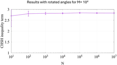
Figure 4. The CHSH values for a system of coordinates rotated such that we have $j=0$ for all four terms of the CHSH inequality and $j^{\prime }$ rotated appropriately to obtain the angle differences $j^{\prime }-j$ as used in Aspect-type experiments. Note that the CHSH inequality is always significantly violated, with a value close to the quantum result.

As clearly seen in Figure 4, the rotation of the polarizer angle-pairs has completely destroyed the validity of the CHSH inequality. Therefore, the CHSH inequality is not invariant to rotations of the polarizer angle-pairs and the coordinate system as is required by the results of quantum mechanics and by a world of experimental evidence including the classical limit for very large numbers of photons.

8 Conclusion

We have used the Fundamental Model of probability theory (Williams, 2001) for experiments using single photons or photon-pairs and polarizers in two very different configurations, one corresponding to Malus-type measurements, the other to EPRB-type measurements such as performed by Kocher and Commins (1967) and groups related to Aspect (2015), Clauser et al. (1969) and Kwiat et al. (1999); Giustina et al., 2015).

Our model shows a pronounced violation of the Bell-CHSH inequalities and agreement with the quantum result. We have shown that this unexpected violation of the highly respected inequalities arises, within the confines of the Fundamental Model (Williams, 2001), from the fact that there are precise premises that guarantee the mathematical validity of the inequalities. However, these mathematical premises lead to a mathematical-physical problem: The correctly derived Bell-CHSH inequalities are physically not acceptable, because they are not invariant to rotations of the polarizer-angle pairs. This lack of invariance makes Bell-CHSH physically unacceptable as a model for the actual experiments such as (Kocher and Commins, 1967; Clauser et al., 1969; Aspect, 2015; Kwiat et al., 1999; Giustina et al., 2015), which are invariant to such rotations. The paradox created by the work of Bell is, thus, resolved and proven to be no reason to suspect any failure of Einstein’s separation principle as well as the ideas of Einstein and ‘t Hooft ('t Hooft, 2020; 't Hooft, 2024) regarding the existence of ontological hidden variables and their local-causal nature.

Data availability statement

The original contributions presented in the study are included in the article/supplementary material, further inquiries can be directed to the corresponding author.

Author contributions

KH: Writing–original draft, Writing–review and editing, Conceptualization, Formal Analysis, Methodology, Visualization. JK: Writing–review and editing, Methodology, Software, Validation, Visualization.

Funding

The author(s) declare that no financial support was received for the research and/or publication of this article.

Acknowledgments

Recent correspondence with Anthony J. Leggett has been a very valuable motivation for us to derive Theorems 1 and 2. While we agree on the importance of the cardinality, the Theorems may explain at least some of the differences of our views mentioned in (Leggett, 2024). Comments of Colin Naturman regarding finite subsets and subtleties for a countable-infinite number of elements of physical reality were helpful for our formulation of the Theorems. We also thank the referees for their important contributions to the clarity of the explanations.

Conflict of interest

The authors declare that the research was conducted in the absence of any commercial or financial relationships that could be construed as a potential conflict of interest.

The author(s) declared that they were an editorial board member of Frontiers, at the time of submission. This had no impact on the peer review process and the final decision.

Generative AI statement

The author(s) declare that no Generative AI was used in the creation of this manuscript.

Publisher’s note

All claims expressed in this article are solely those of the authors and do not necessarily represent those of their affiliated organizations, or those of the publisher, the editors and the reviewers. Any product that may be evaluated in this article, or claim that may be made by its manufacturer, is not guaranteed or endorsed by the publisher.

References

Aspect, A. (2015). Closing the door on Einstein and bohr’s quantum debate. Physics 8, 123. doi:10.1103/physics.8.123

CrossRef Full Text | Google Scholar

Baym, G. (1973). Lectures on quantum mechanics. Redwood City: Adison-Wesley Publishing Company Inc., 1–8.

Google Scholar

Bell, J. S. (1964). On the Einstein podolsky rosen paradox. Physics 1, 195–200. doi:10.1103/physicsphysiquefizika.1.195

CrossRef Full Text | Google Scholar

Clauser, J. F., Horne, M. A., Shimony, A., and Holt, R. A. (1969). Proposed experiment to test local hidden-variable theories. Phys. Rev. Lett. 23, 880–884. doi:10.1103/physrevlett.23.880

CrossRef Full Text | Google Scholar

Einstein, A., Podolsky, B., and Rosen, N. (1935). Can quantum mechanical description of physical reality be considered complete? Phys. Rev. 16, 777–780. doi:10.1103/physrev.47.777

CrossRef Full Text | Google Scholar

Feynman Lectures (1965). Physics 11–14.

Google Scholar

Gisin, N. (2012). Non-realism: deep thought or a soft option? Found. Phys. 42, 80–85. doi:10.1007/s10701-010-9508-1

CrossRef Full Text | Google Scholar

Giustina, M., Versteegh, M. A., Wengerowsky, S., Handsteiner, J., Hochrainer, A., Phelan, K., et al. (2015). Significant-loophole-free test of bell's theorem with entangled photons. Phys. Rev. Lett. 115, 250401–250407. doi:10.1103/physrevlett.115.250401

PubMed Abstract | CrossRef Full Text | Google Scholar

Hess, K. (2023). Logical conflict between Bell’s locality and probability theory. J. Mod. Phys. 14, 1762–1770. doi:10.4236/jmp.2023.1413105

CrossRef Full Text | Google Scholar

't Hooft, G. (2024). The hidden ontological variable in quantum harmonic oscillators. Front. Quantum Sci. Technol. 3, 1505593.

Google Scholar

Jakumeit, J., and Hess, K. (2024). Breaking a combinatorial symmetry resolves the paradox of einstein-podolsky-rosen and Bell. Symmetry 16, 255–265. doi:10.3390/sym16030255

CrossRef Full Text | Google Scholar

Khrennikov, A. (2009). “Contextual approach to quantum formalism,” in Fundamental theories of physics. Springer Nature.

Google Scholar

Kocher, C. A., and Commins, E. D. (1967). Polarization correlation of photons emitted in an atomic cascade. Phys. Rev. Lett. 18, 575–577. doi:10.1103/physrevlett.18.575

CrossRef Full Text | Google Scholar

Kupczynski, M. (2020). Is the moon there if nobody looks: Bell inequalities and physical reality. Front. Phys. 8, 1–13. doi:10.3389/fphy.2020.00273

CrossRef Full Text | Google Scholar

Kwiat, P. G., Waks, E., White, E. G., Appelbaum, I., and Eberhard, P. H. (1999). Ultrabright source of polarization-entangled photons. Phys. Rev. A 60, 773–776. doi:10.1103/physreva.60.r773

CrossRef Full Text | Google Scholar

Leggett, A. J. (2024). The EPR-bell experiments: the role of counterfactuality and probability in the context of actually conducted experiments. Philosophies 9.5, 133. doi:10.3390/philosophies9050133

CrossRef Full Text | Google Scholar

't Hooft, G. (2020). Deterministic quantum mechanics: the mathematical equations. Front. Phys. 8. doi:10.3389/fphy.2020.00253

CrossRef Full Text | Google Scholar

Vorob’ev, N. N. (1962). Consistent families of measures and their extension. Theory Probab. Its Appl. 7, 147–163.

Google Scholar

Williams, D. (2001). 44. Cambridge: Cambridge University Press, 73–110.

Google Scholar