 Carl A. Kocher
- Quantum Foundry, University of California, Santa Barbara, Santa Barbara, CA, United States
The first experimental observation of entangled visible light was achieved by optically exciting free atoms of calcium and detecting pairs of photons emitted in a two-stage cascade. The polarizations of the entangled photons were observed to be correlated, in agreement with quantum theory. This review describes the rationale, methodology, challenges, and results, including experimental details not previously published.
1 Introduction
In the mid-1960s, as a young experimental physicist at the University of California, Berkeley, I was fascinated by quantum theory and impressed by its success in describing small systems such as atoms and molecules. Of particular interest was the 1935 article by Einstein, Podolsky, and Rosen (Einstein et al., 1935), which notes that if particles have a common origin, measurements of their properties (such as spin states) may be correlated. The correlation remains, even if the particles move apart and are spatially separated. In this hypothetical situation, quantum effects would be apparent on a macroscopic scale.
Although the term “entanglement” was coined by Schrödinger in the 1930s, it was not in common use in the 1960s. In simple terms, entanglement is a property of a system containing two or more particles, in which the quantum state of a particle depends on, and is linked to, the states of others. Electrons, for example, are entangled in every atom, every molecule, every material. So it would be fair to say that entanglement is everywhere. And experiments on entangled systems can reveal aspects of Nature that may seem surprising and quite remarkable.
I was interested in finding the simplest possible system for studying the effects of entanglement, and began feasibility studies for a low-energy experiment that could be set up in a small laboratory with a limited budget. Inspired by the Einstein-Podolsky-Rosen gedanken experiment, it would deal with the spin states of just two entangled particles.
If the particles were electrically charged, like low-energy electrons, there would be no clean way to extract them without exposure to stray fields that would affect the spins. Therefore it seemed natural to consider visible light, in which the photons have no charge and are non-interacting. When atoms emit light, there is no need to extract the photons: Nature performs the extraction process for us.
2 Experimental concept
If a free atom is excited, it can make a transition to a lower-energy state, via the spontaneous emission of electromagnetic radiation in the form of a photon. Although the photon may be detected as a point-particle, it propagates as an extended wave packet, spreading as it moves out from the atom, carrying angular momentum (spin) as well as energy.
Figure 1 shows several singlet-state energy levels for an isolated calcium atom. If the atom is initially in state A, it can give up energy in two stages, A → B and B → C, with the emission of Photon 1 (green light, 551 nm) and Photon 2 (violet light, 423 nm). The corresponding spectral lines are seen in the emission spectrum of calcium.
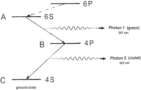
Figure 1. Photons emitted in a two-stage cascade.
An ensemble of excited calcium atoms is shown at the center of Figure 2, with the green and violet photons detected by photomultiplier detectors (PM) along a common axis.
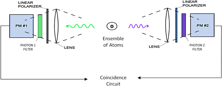
Figure 2. Experimental geometry, simplified.
Narrow-band interference filters pass the desired wavelengths while blocking other light. Pulses from the detectors are recorded as atoms proceed through the two-stage cascade A → B → C. For identification of photon pairs from the same atom, the detector pulses can be fed into a coincidence circuit that “clicks” only when photons arrive at the two detectors at nearly the same time.
Since light propagates as a wave, even in the quantum realm, the experiment can incorporate familiar optical components such as lenses, interference filters, linear polarizers, and glass vacuum windows, through which the photons can pass prior to detection.
The spin state of a photon corresponds to its polarization state, as noted in Section 3.2, where the two-photon final state is discussed. In the visible region of the spectrum, polarizations can be studied with ordinary linear polarizers, commonly known as Polaroid sheets. In the experiment, a rotatable linear polarizer is mounted in front of each detector, so that the coincidence counting rate can be recorded as a function of the angular orientations of the polarizers.
This experiment would be the first attempt to count and analyze single optical photons and pairs of photons emitted in an atomic cascade. (Kocher, 1967a; Kocher and Commins, 1967).
Why did I choose calcium? 1) Efficient linear polarizers are available for polarization measurements at the green and violet calcium wavelengths. 2) Single-photon detection by photomultiplier detectors is possible, although somewhat inefficient, for light at these wavelengths. 3) Entanglement calculations are simple and unambiguous for calcium, as the initial and final states, A and C, are spherically symmetric. Spherical symmetry requires that all internal angular momenta for the atom (orbital, electron spin, and nuclear spin) must be zero. States A and C are S-states, with no orbital angular momentum. Zero electron spin suggests an atom from the second column of the periodic table, with two valence electrons forming singlet states for which the spins cancel. It is also fortunate that essentially all the atoms in naturally occurring Ca (99.8%) have spin-zero nuclei. 4) The vapor pressure characteristics of calcium allow for the production of an atomic beam from a suitable oven in a vacuum chamber.
3 Relevant quantum concepts
This section presents, in simplified form, a view of the theoretical background for the entanglement of photon polarization states.
3.1 Polarization measurements
A linear polarizer is an anisotropic flat plate with a transmission axis in its plane. In the classical domain, in which light behaves as a transverse electromagnetic wave, linearly polarized light passes undiminished through an ideal polarizer if its axis is parallel to the electric field in the wave. However, no light is transmitted if the electric field and polarizer directions are perpendicular. The meaning of “no light” can be extended to the quantum realm, where it means “no photons” are transmitted. Thus it is possible to regard the polarizer as a filter for quantum states.
In Figure 3, light travels along the experiment’s axis of symmetry, shown here as the z-axis, with a linear polarizer in the xy plane. Capital letter X will denote the photon state transmitted by a polarizer aligned along the x-axis, and similarly Y for the y-axis. The general polarization state Ψ for a single photon is a linear combination, or coherent mixture, of these states:
where ax and ay are amplitudes (in general, complex) that tell how much of each state is present in the admixture.
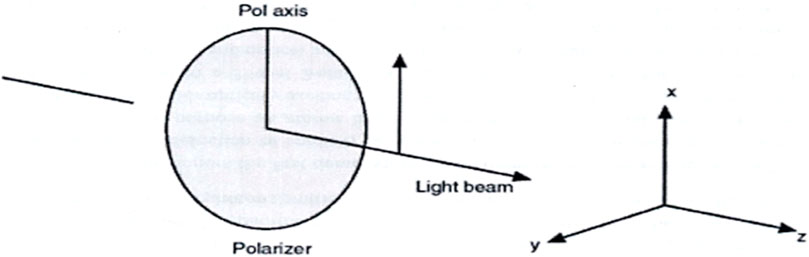
Figure 3. Linear polarizer geometry.
Quantum theory provides two ways for the state of a system to change in time:
(1) The Time-dependent Schrödinger Equation is central to quantum mechanics. Solving it yields a wave function or state vector Ψ(t) that describes the system and its continuous evolution between measurements.
(2) The Reduction Postulate determines how Ψ changes when a measurement is made. A measurement leads to a sudden collapse, or projection, of Ψ onto the observed state.
The state Ψ for a photon therefore changes discontinuously as a result of a polarization measurement. If the photon described by Eq. 1 is detected after passing through a polarizer with its transmission axis along x, that constitutes a measurement. In this case the reduction postulate requires that the Y term must drop out. Only the observed-state X term remains in Ψ after the measurement.
The experiment in Figure 2 explores the reduction postulate in a two-photon system.
3.2 Polarization states for entangled photons
Photon spin states for light traveling in the z-direction can be expressed in terms of linear polarization states X and Y (as above), or in terms of helicity. The two sets of basis states are related as follows (with normalization factors not shown):
Spin parallel to photon momentum:
Spin antiparallel to photon momentum:
Conservation laws for angular momentum and parity play a central role in quantum correlation phenomena. For the three-level radiative cascade in Figure 1, the initial atomic state A and final state C both have zero total angular momentum and even parity. Therefore, the two-photon final state Ψ must also satisfy the conditions of zero angular momentum and even parity:
If the same z-axis is used for both photons and is directed to the right in Figure 2, the states for Photon 1 require i → - i. Then
in which the X1·Y2 and Y1·X2 terms drop out, yielding (without normalization factor) a simple and elegant result
for the two-photon system, before either photon is detected. The reasoning in Eqs 2, 3, leading to Eq. 4, gives it a sense of universality, as no consideration is given to the internal structure of the source atom or its interaction with a quantized radiation field. Before any measurements have been made, each photon has a potential to pass through a linear polarizer with any orientation.
The two-particle quantum state Ψ is not a simple product, as it would be for photons having no common history. Instead it is a sum of products representing an entangled state. Entanglement of the photons is evident in Eq. 4, where neither photon has an independent identity. In each of the two terms, the amplitude for one of the photons is a wave function for the other.
Since the orientation for the x- and y-axes around z is arbitrary, the form of Eq. 4 will remain unchanged if the xy coordinate system is rotated through any angle about the z-axis.
3.3 Polarization correlation
If the first photon (green) passes through a linear polarizer transmitting the state X1, the reduction postulate removes the second term, containing Y1, from Ψ in Eq. 4. Only the first term remains, leaving the second photon (violet) unambiguously in polarization state X2. More generally, if one of the photons passes through a linear polarizer at any orientation, the remaining photon will then be in the same polarization state, pending future measurements.
Quantum theory makes specific predictions for the experiment shown in Figure 2.
(1) If both polarizers are aligned with their axes parallel, coincidence counts will be observed.
(2) If the polarizer axes are perpendicular, no coincidences will be observed—a conclusion that also follows directly from the absence of cross-terms X1·Y2 and Y1·X2 in Eq. 4. This signature of entanglement, which has no classical analog, is noteworthy and accessible to experimental observation.
These predictions may seem counterintuitive, bizarre, or weird, especially because there is no known evidence for physical transmission of information from one detector to the other. This question is addressed further in Section 6.
Additional remarks:
(a) Taken separately, the green and violet beams are unpolarized.
(b) If there is a general angle between the polarizer axes, Eq. 4 predicts a coincidence probability (and therefore a counting rate) that varies as the square of the cosine of this angle.
(c) The reduction postulate also enables calculations of the time dependence for the detection of entangled photons emitted by an atom. (Kocher, 1971).
4 Experimental considerations
4.1 Photon detection
A photomultiplier detector is an evacuated and sealed glass tube with a light-sensitive cathode on a window at one end. As Einstein first realized, the energy of a detected photon is conveyed to a single photoelectron from the cathode. This electron is accelerated toward a positively charged metal dynode, where additional electrons are knocked loose. This process is repeated at additional dynodes, producing a negative pulse that can be counted with standard electronics. Quantum efficiencies (output pulse probability per photon) are of order 10% (green) to 20% (violet). Photoelectrons released from different locations on the cathode travel a range of distances in reaching the first dynode, introducing some loss of time resolution, typically several nanoseconds. In addition, thermal processes can release electrons randomly from the cathode, resulting in spurious output pulses, or “dark noise.”
4.2 Atomic beam oven
The oven, shown in Figure 4, is 6.5 cm in length and machined from tantalum, a nonreactive refractory metal. It is heated by an electric current through internal resistive coils. A cylinder of calcium metal is loaded into the well. When the oven is installed in a vacuum chamber and heated, monatomic calcium vapor evaporates from the solid and comes out through an opening in the front, forming a beam.

Figure 4. Atomic beam oven for calcium.
A thermocouple junction, set into a small hole in the oven, reads out the temperature. At 1000 K, an oven load of Ca (12 g) will empty in about 25 h, and a typical beam velocity for a Ca atom is about 105 cm/s. Since the radiative cascade requires about 10–8 s, the atom moves only about 10–3 cm—a negligible distance—while the photons are being emitted.
The oval at the center of Figure 2, labeled “Ensemble of Atoms,” represents a cross section of the atomic beam from this oven.
4.3 Excitation strategy
The two-stage cascade, as shown in Figure 1, requires excitation of calcium atoms from the 4S ground state to the 6S excited state. This is a challenging problem, since the direct 4S → 6S transition is “forbidden” for single-photon absorption. (Dipole matrix elements are zero.) An acceptable alternative would be to optically excite the 6P state (also shown in Figure 1) by an allowed transition, 4S → 6P. The 6P can decay to 6S by emitting an infrared photon that is not observed, and then the desired cascade can take place. The 4S → 6P excitation requires a 228 nm ultraviolet light source.
A minor complication is that while the 6P state can decay to 6S, it can also decay to 5S and several D-states (in total about 8 times as likely as 6S). All of these return to the ground state via the 4P state, producing a Photon 2 not time-correlated with a Photon 1. Detector pulses from unpaired violet photons can trigger false coincidences and are a source of noise.
In 1964 it was a major challenge to find an acceptable 228 nm UV excitation source for the 4S → 6P transition. No tunable lasers, UV lasers, or UV LEDs were available. (There were also no pocket calculators and no lab computers. It was still the slide rule era.)
A calcium discharge lamp could not be considered as a 228 nm source, as it would produce intense 423 nm (violet) radiation that could not be effectively blocked from reaching the Photon 2 detector. Electron impact excitation would pose a similar problem. A third possibility was a continuum source of ultraviolet light, in conjunction with a 228 nm bandpass interference filter. A high-pressure mercury lamp was considered, but even this produced far too much visible light.
Then I read about the UV continuum emitted by molecular hydrogen, with wavelengths spanning the range from about 180 nm to 450 nm. No suitable lamps were commercially available, so I designed and built a cylindrical low-voltage high-current H2 arc lamp in a brass chamber, using a porous tungsten dispenser cathode and a continuous flow of H2 gas. (Kocher, 1967b). This turned out to be essential to the eventual success of the experiment. The lamp operated at 17 V, 30 amps, with the discharge produced between the cathode and anode in the cross-sectional view of Figure 5. Fused quartz transmits 228 nm radiation, so a quartz focusing lens is mounted between the lamp and the excitation region.
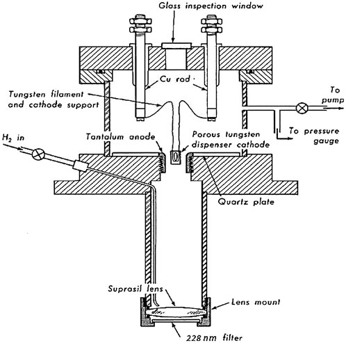
Figure 5. 500 watt H2 arc lamp.
If the broadband UV light were applied perpendicular to the Ca beam, only atoms within the natural linewidth (about 30 MHz) for the 4S → 6P transition could be excited, and all the useful radiation would be absorbed near the edge of the atomic beam. Atoms beyond this edge would not be excited. However, there is a spread in atomic velocities from a thermal oven, and the Doppler-broadened linewidth (1,000 MHz) exceeds the natural linewidth by a factor of about 30. In the experimental plan I therefore introduced the calcium beam at 45° relative to the observation z-axis, from lower left to upper right in Figures 2 and 6. With this configuration the much larger number of atoms in the Doppler-broadened absorption line can potentially be excited to the 6P state. The oblique angle between the atomic beam and the detector axis also effectively eliminates trapping and multiple scattering of the emitted 423 nm violet photons.
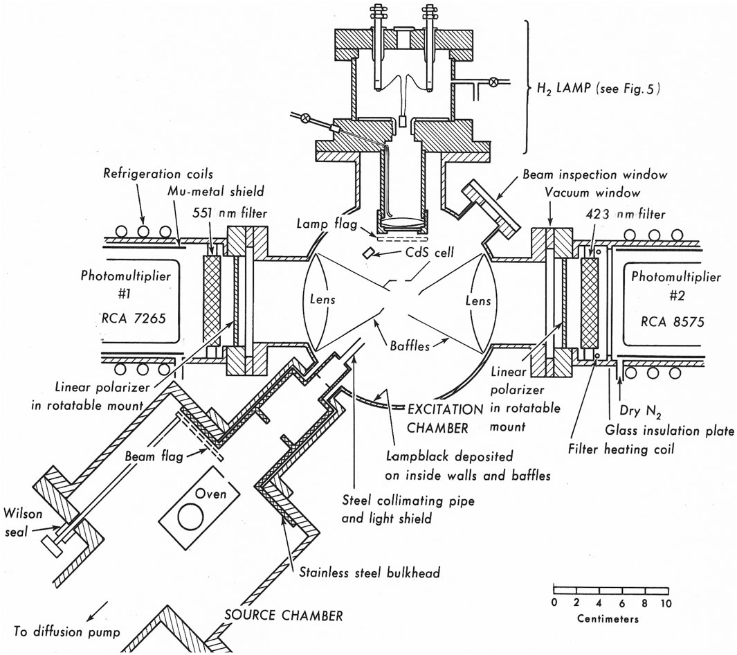
Figure 6. Cross section of the apparatus, top view.
4.4 Coincidence rate estimate
It would not be wise to proceed with a complex experiment unless the signal and noise levels can be estimated. Therefore, before the major construction of a vacuum chamber and dealing with pumps, hoses, ion gauges, etc., an effort was made to calculate the coincidence counting rate under reasonable experimental conditions.
For each detector I considered the fractional solid angle of intercept, together with the quantum efficiency and the filter transmission, and found that about 106 cascade-emitting atoms are needed for each observable coincidence count—without the polarizers.
The atomic beam oven holds about 1023 atoms of Ca, but only 1 atom in 103 would pass through the excitation region.
I used a radiation thermopile to measure the intensity of the H2 arc lamp in conjunction with a 228 nm bandpass filter. I also searched the literature for transition rates in calcium and determined the branching ratios for the transitions.
It was a complex process putting these pieces together, attempting to identify every limitation and concern. In the end I estimated 1 coincidence per second (with the polarizers removed), with an uncertainty factor of about 5.
Under these conditions, reasonable statistics—and a clear experimental result—might be obtained with a multi-hour observation. It would be a difficult undertaking, requiring considerable care, patience, a long observation time, and some courage.
4.5 Apparatus details
The experimental plan employs a vacuum system with two diffusion-pumped brass chambers and removable flanges for access. A water-cooled source chamber holds the calcium beam oven. The excitation chamber, pumped to a lower pressure (10–6 Torr), contains the interaction region, where UV light from the H2 lamp would excite Ca atoms in the atomic beam, and from which the green and violet photons would be detected by photomultiplier assemblies outside the chamber.
Details of the experiment are shown in Figure 6 and in a photograph, Figure 7.
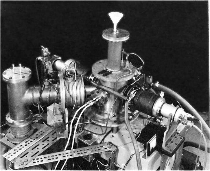
Figure 7. Apparatus photograph corresponding to Figure 6.
It took more than a year to reach the point where all the parts of the experiment could be assembled. The components were tested separately, to the extent possible, and then in tandem.
Two flags, shown in Figure 6, can be controlled from outside the chamber. One can block the calcium beam, and the other can block the UV radiation from the lamp so it cannot reach the beam. This flexibility made it possible to monitor and optimize the counting rate for each detector separately. It was then possible to determine the sources of extraneous coincidence counts, of which there were many, including stray light from the oven heating coils and visible-light fluorescence due to the UV from the lamp. I installed light-blocking baffles and applied lampblack to the chamber walls. The improvements were slow and incremental.
After this was done, photomultiplier “dark noise,” which had always been present, became noticeable at room temperature. To address this problem, I cooled the photomultipliers by soldering a helix of copper tubing around each brass photomultiplier enclosure and installing a refrigeration compressor that could circulate refrigerant through the tubing. The photocathode temperatures were cooled to −15°C, reducing the dark noise significantly.
Instead of using a simple coincidence circuit, I recorded coincidence counts versus the time delay between the pulses from the two detectors, using a time-to-pulse-height converter and a multichannel pulse-height analyzer, as in Figure 8.
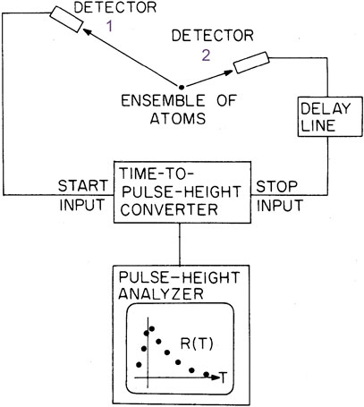
Figure 8. Basic electronics for recording and displaying coincidence counts.
The time-to-height converter produces an output pulse with an amplitude proportional to the time delay between the “start” pulse (from the Photon 1 detector} and the “stop” pulse (from the Photon 2 detector). A pulse-height analyzer stores these counts in an array of magnetic-core memory channels corresponding to a span of delay times. Each memory channel effectively represents a separate coincidence circuit, for which the time spread can be varied by changing the ramp rate. The time offset, corresponding to sliding the distribution to the right or left, can be adjusted by varying a delay line (a length of coaxial cable) on the Photon 2 side.
If the pulse pairs are from the same atom, they contribute to a central peak in the distribution, as viewed on an oscilloscope. Pulse pairs may also be due to photons from different atoms, or to stray light. In these cases the time intervals are random, contributing to a background signal, with fluctuating statistics, along the entire horizontal time scale.
5 Final testing and results
Figure 9 shows the laboratory in 1966. Test runs were attempted with the calcium beam and H2 lamp running, without the polarizers. As expected, the Photon 2 detector recorded the most photons, and the single-detector counting rates increased encouragingly when the beam and the UV excitation were both on. Unfortunately the rate for coincidence counts was lower than the lower limit I had estimated, by a factor of about 10. Under these conditions the experiment could not yield clear results.
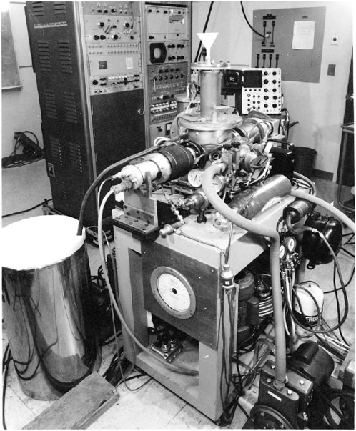
Figure 9. Overall view of the experiment.
Weeks passed, with considerable frustration, and I went into a deep search for an explanation. All questions had to be asked, and everything rechecked. Then I thought of a possible reason for the low coincidence rate. An interference filter was mounted on each photomultiplier assembly. These were high quality narrow-band filters, made from sets of dielectric plates and built-to-order for the calcium wavelengths. But dielectrics tend to be thermally sensitive, and I now realized that when I installed the refrigeration coils for cooling the photomultipliers, I also ended up cooling the filters. If the filters were thermally sensitive, the transmitted wavelength could have shifted. If the shift were large enough, the filter would end up being “tuned off-resonance” and the desired wavelength would be blocked instead of transmitted.
I removed the filters, got a bucket with dry ice, a thermometer, and some clean rags, and scanned the filters using a recording spectrophotometer. I started with the filters at room temperature and printed out the scans. The peak wavelengths were very close to what I had ordered, at 551.3 nm and 422.7 nm. Then I wrapped the filters, cooled them with dry ice to −20°C, and made repeated spectrometer scans as they warmed up. The violet filter, which had the narrower passband, was far off resonance at −20°C and also at −10°C. To correct for this shift I added a small heating coil for the violet filter and adjusted the current through it to bring the filter’s transmission peak back onto the wavelength for the violet-light photons. This is shown in Figure 6.
Then I loaded the oven with a full cylinder of calcium and pumped down the vacuum system. A clear, unequivocal coincidence signal was apparent within an hour. That afternoon I obtained the time correlation plot in Figure 10, showing coincidences in the form of a peak.

Figure 10. Coincidence counts displayed from memory of pulse-height analyzer.
Here the horizontal separation between channels represents a time interval of 0.8 ns. The exponential decay of the 4P state, which has a mean lifetime of 4.5 ns, shows up as an asymmetry, although each photomultiplier smears out the time resolution by about 3 ns. The counts above the noise baseline are coincidences.
As noted previously, the separate Photon 1 and Photon 2 light beams are expected to be unpolarized. To check this I installed the polarizers and verified that the single-detector counting rates did not vary with the polarizer orientations.
Finally, a 25-h run with the polarizers installed, on December 17 and 18, 1966. The experiment continued through the night, with data recorded during 21 consecutive hours. Parallel and perpendicular polarizer configurations were alternated, with the recording of data switched in cycles between memory banks for horizontal and vertical polarizer combinations xx, yy, xy, and yx. Equal recording periods were allotted to parallel and perpendicular orientations of the polarizers. The results are shown in Figure 11, where each point represents a sum over three adjacent analyzer channels. Upper panel (A) shows a coincidence peak with the polarizer axes parallel. Lower panel (B) shows no peak with the axes perpendicular.
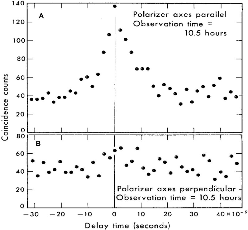
Figure 11. Experimental Results: Coincidence counts recorded as a function of delay time: (A) With the polarizer axes parallel, a clear coincidence peak is observed, and (B) With the polarizer axes perpendicular, no peak is present.
The hint of a peak in (B) can be attributed entirely to the imperfect linear polarizers, which transmitted 6% of unpolarized violet light when crossed at 90°.
Most significantly: When the polarizer axes are perpendicular, no coincidences are recorded. This conclusion is in agreement with the predictions of quantum theory for entangled photons.
The photon detectors in this experiment were about 40 cm apart, a macroscopic distance. Each photon is a spherical wave, traveling outward from the atom at the speed of light. Before the photons are detected, their coupled (or entangled) waves occupy the entire space between the atom and the detectors. As a consequence the quantum system is macroscopic, with the two-photon wave function extending over a macroscopic region.
When this work was undertaken it was inconceivable that, decades later, unforeseen and breathtaking developments, including sophisticated lasers and parametric down-conversion, would enable the creation of entangled photons in great numbers, or that they might play a role in practical or useful technology. Yet we now understand that entanglement and quantum correlations can be exploited, leading to an exciting new field of “quantum information.”
6 Reflections and overview
In an experiment with non-interacting particles, how can a measurement here affect what happens there? It may seem profoundly strange that quantum theory—the best we have—does not introduce or incorporate a deterministic “causal mechanism” for correlations in the measurements. Could there be some identifiable process that allows one photon, or one measurement, to communicate with the other?
Einstein famously called these kinds of effects “spooky action at a distance.” What is now known as the “Einstein-Podolsky-Rosen paradox” led him to suggest that the theory might be “incomplete” in some way. Nevertheless the quantum theory of the 1920s and 30s does accurately predict and describe experimental results, including entanglement phenomena. It is a successful theory that has been tested repeatedly, including by others who used my apparatus years later and confirmed the results presented here. (Freedman and Clauser, 1972).
Could there be situations where quantum theory makes incorrect predictions, or where alternative theories give equally satisfactory explanations? Much effort has been devoted to theories involving hidden variables and to experiments probing the Bell inequalities. Yet none of these, so far, appear to have led to new physics.
Most of us have never lived in an overtly quantum world, and so it is tempting to proclaim a “paradox” when expectations based on classical phenomena are extrapolated into the quantum realm. A corollary might be offered—that credible experiments yielding strange results should be welcomed into our consciousness, celebrated for their insight, and incorporated into the life experience from which intuition derives.
From my perspective, performing an experiment of this kind was a rare opportunity for witnessing a strangely wonderful quantum phenomenon and bringing it into the domain of experience. It is a search for truth, and if the truth changes our outlook on the world, so much the better.
Data availability statement
The original contributions presented in the study are included in the article/Supplementary Material, further inquiries can be directed to the corresponding author.
Author contributions
CK: Conceptualization, Data curation, Investigation, Methodology, Writing–original draft, Writing–review and editing.
Funding
The author declares that no financial support was received for the research, authorship, and/or publication of this article.
Acknowledgments
Eyvind Wichmann, a theoretician, is gratefully acknowledged for inspiring this project. While planning a curriculum in quantum physics for second-year undergraduates, he conceived an original idea for the instructional laboratory: a “tabletop experiment” for observing the polarizations of atomic cascade photons. I remember his words: “I have one new idea, but I don’t know if it can be done.”
Eugene Commins, a splendid collaborator and an outstanding teacher, was immediately receptive to this experiment when I proposed that we work on it together. With a unique gift for conveying complex ideas with clarity and humor, Gene offered much encouragement, arranged my access to equipment from LRL, and provided $10,000 to cover all the expenses for the experiment.
John Clauser came to Berkeley several years after this experiment was completed, and used my apparatus, with minor improvements, in a test of the Bell inequalities. In the process, he repeated my experiment and verified the results as presented here. Not every research endeavor has the benefit of independent confirmation.
Conflict of interest
The author declares that the research was conducted in the absence of any commercial or financial relationships that could be construed as a potential conflict of interest.
Publisher’s note
All claims expressed in this article are solely those of the authors and do not necessarily represent those of their affiliated organizations, or those of the publisher, the editors and the reviewers. Any product that may be evaluated in this article, or claim that may be made by its manufacturer, is not guaranteed or endorsed by the publisher.
References
Einstein, A., Podolsky, B., and Rosen, N. (1935). Can quantum-mechanical description of physical reality be considered complete?. Phys. Rev. 47, 777–780. doi:10.1103/PhysRev.47.777
Freedman, S. J., and Clauser, J. F. (1972). Experimental test of local hidden variable theories. Phys. Rev. Lett. 28, 938–941. doi:10.1103/PhysRevLett.28.938
Kocher, C. A. (1967a). Polarization correlation of photons emitted in an atomic cascade. UCRL Report 17587, 79. Available at: https://escholarship.org/uc/item/1kb7660q.
Kocher, C. A. (1967b). Metal-cased H2 arc lamp of simplified design. Rev. Sci. Instrum. 38, 1674–1675. doi:10.1063/1.1720643
Kocher, C. A. (1971). Time correlations in the detection of successively emitted photons. Ann. Phys. 65, 1–18. doi:10.1016/0003-4916(71)90159-X
Keywords: entanglement, EPR paradox, atomic cascade, photon counting, reduction postulate, polarization correlation, Bell inequalities
Citation: Kocher CA (2024) Quantum entanglement of optical photons: the first experiment, 1964–67. Front. Quantum Sci. Technol. 3:1451239. doi: 10.3389/frqst.2024.1451239
Received: 18 June 2024; Accepted: 01 July 2024;
Published: 22 August 2024.
Edited by:
Karl Hess, University of Illinois at Urbana-Champaign, United StatesReviewed by:
Bengt Norden, Chalmers University of Technology, SwedenJuergen Jakumeit, Access e.V., Germany
Copyright © 2024 Kocher. This is an open-access article distributed under the terms of the Creative Commons Attribution License (CC BY). The use, distribution or reproduction in other forums is permitted, provided the original author(s) and the copyright owner(s) are credited and that the original publication in this journal is cited, in accordance with accepted academic practice. No use, distribution or reproduction is permitted which does not comply with these terms.
*Correspondence: Carl A. Kocher, a29jaGVyQG1haWxhcHMub3Jn