Quantum computers, quantum computing, and quantum thermodynamics

Quantum thermodynamics aims to extend standard thermodynamics and non-equilibrium statistical physics to systems with sizes well below the thermodynamic limit. It is a rapidly evolving research field that promises to change our understanding of the foundations of physics, while enabling the discovery of novel thermodynamic techniques and applications at the nanoscale. Thermal management has turned into a major obstacle in pushing the limits of conventional digital computers and could also represent a crucial issue for quantum computers. The practical realization of quantum computers with superconducting loops requires working at cryogenic temperatures to eliminate thermal noise, and ion-trap qubits also need low temperatures to minimize collisional noise. In both cases, the sub-nanometric sizes also bring about the thermal broadening of the quantum states; and even room-temperature photonic computers eventually require cryogenic detectors. A number of thermal and thermodynamic questions, therefore, take center stage, such as quantum re-definitions of work and heat, thermalization and randomization of quantum states, the overlap of quantum and thermal fluctuations, and many others, even including a proper definition of temperature for the small open systems constantly out of equilibrium that are the qubits. This overview provides an introductory perspective on a selection of current trends in quantum thermodynamics and their impact on quantum computers and quantum computing, with language that is accessible to postgraduate students and researchers from different fields.

1 Introduction

Quantum computing has gone a long way from the dream of Richard Feynman expressed in his keynote article of 1982 (Feynman, 1982) to the increasingly sophisticated theoretical developments that followed in the 1990s to the first realizations of experimental quantum bits in the past 20 years (Huang et al., 2020; Editorial, 2022; Pelucchi et al., 2022). Today, we are only starting to see the first true quantum machines sporting some tens of qubits connected by fully reversible quantum gates, which attempt to solve theoretical benchmark challenges. They do not yet calculate real-life problems; however, they are getting a bit closer every few months on a path that seems to echo the spectacular growth of digital microelectronics in the last half of the past century.

Looking at the latest developments among the main players in quantum hardware and software, Google’s Quantum-AI subsidiary Alphabet first reported having reached “quantum advantage” in July 2019 with their Sycamore machine (Arute et al., 2019), a claim later challenged by IBM engineers (see below). Both IBM and Google use qubits made with superconducting loops. IBM has already broken the 100-wall with its 127-qubit Quantum Eagle (Kim et al., 2023) and recently announced its new milestone by the end of 2023 with the QuantumSystem-Two modular architecture, which includes three Heron 133-qubit devices. Intel is also engaged in both superconducting and spin qubit research studies: in June 2023, they unveiled its new TunnelFalls, a 12-qubit all-silicon chip. NVIDIA launched the DGX Quantum, a GPU-accelerated system, integrating their GraceHopper superchip with the OPX platform by Quantum Machines in March 2023. Honeywell opted for trapped-ion qubits in their System-Model H1, the 10-qubit first operational machine, already used for quantum chemistry simulations (Yamamoto et al., 2024), a similar road to that followed by IonQ with their Aria 25-qubit machine. Microsoft chose to work with a different concept for their Azure quantum system, the “topological” qubits (Aghaee et al., 2023), for which they received DARPA support; however, they also pursued a different, hybrid strategy by coupling qubit-virtualization with ion-trap physical qubits from Quantinuum, to achieve extremely low error rates (da Silva et al., 2024). Notably, all these companies are making their computing platforms, or a scaled-down version thereof, publicly web-accessible to anybody for testing and running quantum codes via the internet.

In June 2022, the US Senate passed the $250 billion Innovation and Competition Act, promoting quantum information technologies among the actions to ensure that the US semiconductor and information technology continue to play a leading role in the global economy. At the other shore of the Pacific, with the help of a multi-billion-dollar funding package and a €10 billion investment in a quantum information laboratory, China hopes to make significant breakthroughs in the field by 2030. Big names such as Alibaba and Baidu are engaged in sustaining R&D (although Alibaba’s quantum laboratory was suddenly shut down in Nov. 2023). Already, one team at the University of Science and Technology of China in Hefei reported achieving quantum advantage by using two radically different technologies, linear optics or superconducting qubits, only 1 year apart from each other (Wu et al., 2021; Zhong et al., 2021).

In Europe, the European Commission launched the “Quantum Technologies Flagship” program to support hundreds of quantum science researchers over a 10-year period with a budget of €1 billion in October 2018. The OpenSuperQPlus project is a medium-term, 4-year project centered at the Jülich Research Center in Germany, assembling 28 partners from 10 EU countries. However, compared to the US and China markets, which are dominated by a few hi-tech giants, the EU panorama is richer in smaller partnerships and smaller companies (Räsänen et al., 2021). The United Kingdom, sadly no longer part of the European Union, has announced conspicuous investments while initially relying on technology provided by the US start-up Rigetti and other local solutions such as the OQC company in Oxford developing their “coaxmon” (Rahamim et al., 2017). As usual, other EU countries are proceeding to work both sides of the street, partly following EU guidelines and partly pushing national initiatives. Germany follows a strategy similar to the United Kingdom, coupling €3 billion in national investment with US quantum technology imported from IBM. The Netherlands launched its national quantum strategy in 2019 with €615 million and the Quantum Delta NL initiative to help quantum research and marketing in universities. France follows, as it often happens, a more original way, with a 5-year €1.8 billion funding initiative (half of which coming from public money), the development of a large-scale quantum annealer (a somewhat different concept from the gate-based quantum computer) by the start-up company Pasqal (Schymik et al., 2022), and, in parallel, the recently announced Quandela (Somaschi et al., 2024) photonic computer installed in the north of France.

So, why thermodynamics? Heat dissipation has always been a crucial problem for digital computers and probably represents the biggest limit to a further expansion of CMOS-based computing technology (Kish, 2002; Valavala et al., 2018; Bespalov et al., 2022). Up to the 1990s, the solution was to reduce the voltage levels, but now we are at 0.7 V, and this figure could not be reduced further. The heating problem has been exacerbated with the introduction of three-dimensional design, which brought with it new issues of capacitive charging of the metal connections crossing in the vertical direction. The progressively reduced transistor dimension, now at limits reaching below 10 nm, has the additional issue of self-heating because of the largely increased surface/volume ratio of the device. Switching is also at its limits: devices in our laboratories can easily function at 100 GHz and more; however, the fastest clock cycle adopted in real computing units cannot go above 5–6 GHz because the rate of heat accumulation cannot be matched by a sufficiently fast rate of dissipation.

Quantum computers might be, in principle, even more sensitive to fluctuations and heat dissipation because qubits are designed at the quantum scale, and the thermal energy can represent a source of noise (interference) in their wavefunction. Discrete energy spectra are typically very sensitive to small perturbations that can break symmetry-related degeneracies. Notably, in order to prepare (reset) and retrieve the information of a qubit, its quantum state must be destroyed, an operation that necessarily entails some heat release. Until now, such a problematic (that is, ensemble of connected problems) has received comparatively little attention because of the already outstanding issues represented by noise from imperfect control signals, interference from the environment, unwanted interactions between qubits, the need for quantum error correction, and the need for operating at cryogenic temperatures. However, questions about temperature, entropy, work, and heat take a very peculiar angle when seen in the context of quantum mechanics and notably quantum computing.

The purpose of this article¹, halfway between a review and a primer, is to give a concise summary of the emerging field of quantum thermodynamics in relation to quantum computing. I should provide a more precise definition at the outset because it may appear an oxymoron to use the word “thermodynamics,” which is the phenomenological theory of the average macroscopic behavior of heat and work exchanges, and the word “quantum” that in itself represents the epitome of the microscopic world, in the same sentence. The two major shortcomings when trying to apply thermodynamics to the quantum domain should be 1) the fact that, by its proper definition, thermodynamics does not contain microscopic information nor does it have a protocol to relate to the microscopic degrees of freedom and 2) the fact that it describes only equilibrium states. The first can be circumvented by passing to the statistical mechanics formulation of thermodynamics, which provides the proper equations and language to link with the microscopic. The solution to the second can leverage on the developments of stochastic thermodynamics, which uses stochastic variables (thus offering a link with the quantum mechanical notion of probability) to describe the non-equilibrium dynamics typically observed at the molecular length and time scales.

Quite obviously, quantum thermodynamics covers more general questions than merely quantum information. Machines that convert heat into electrical power at a microscopic level, where quantum mechanics plays a crucial role, such as thermoelectric and photovoltaic devices, are well-known examples of systems requiring the new language of quantum thermodynamics. It is often said that such machines differ from conventional machines by having no moving parts; however, while they may have no macroscopic moving parts, they function with steady-state currents of microscopic particles (electrons, photons, phonons, etc.), which are all quantum in nature. Nanotechnology has significantly advanced efforts in this direction, offering unprecedented control of individual quantum particles. The question of how this control can be used for new forms of heat-to-work conversion has started to be addressed in recent years (Benenti et al., 2017; Bhattacharjee and Dutta, 2021).

Hence, our title starts with quantum computers and moves to quantum computing, stressing the fact that to realize a quantum computation, you first must build a physical quantum machine. (This is not so obvious because one can also try to simulate the quantum computation on a classical computer.) The role of thermodynamics, and notably of entropy, therefore, will play a dual role in this context, in that it affects both the physical system and the computation that is being carried out on that system. Entropy will have a special position because its different definitions seem to start from rather different premises each time but eventually end up in very similar, if not formally identical, formulations. We will ask whether a formal similarity also implies and to what extent physical identification between different definitions.

This contribution is organized as follows: Sections 2 and 3 give a rapid overview (necessarily incomplete and partial, given the obvious limitations of space) of quantum computers and quantum computing, providing only some basic details to make this article self-contained for the materials that follow. I will mainly focus as a representative example on superconducting loops and the TransMon that, at this stage of development, represent the most popular choice of constructors. Section 4 recalls some notions of basic thermodynamics in the context of digital computers. Section 5 deals with the link between thermodynamic entropy and information entropy and the (ir)reversibility of quantum computations. Section 6 is both the longest and the richest of possibly novel ideas, discussing the reformulation of some classical thermodynamics concepts in the framework of quantum mechanics and providing several examples of key questions in which quantum thermodynamics can make an impact on quantum computing. Some conclusions and outlook are given in the final Section 7.

2 On the advantage of quantum computing

Quantum advantage (the old word to indicate the computational gain of a quantum device compared to a classical digital computer was “supremacy,” but it is currently replaced by “advantage” or “computational advantage”) typically refers to situations in which information processing devices built on the principles of quantum physics attempt to solve computational problems that are not tractable by classical computers. The resulting quantum advantage is usually defined as the ratio of classical resources required to solve the problem, such as time or memory, to the associated quantum resources. Notably, the numerator in this ratio is often only an estimation because the problems that are faced are, by definition, beyond the reach or at the limits of the capabilities of classical digital computers. Quantum thermodynamics will offer an interesting additional perspective by also comparing energy dissipation between classical and quantum computing.

To begin with, some points should be clarified. A quantum computer can use bits and logic gates like a digital computer does. Therefore, at least in theory, it should be able to do any computation a classical computer can do, plus a number of other computations that are beyond classical. From the standpoint of computability theory, the key difference between the two is in the state of the bits at any stage of the computation: a classical bit is always in either one of two defined states; a quantum bit is always in a combined state overlapping with the states of (some or all) the other bits. In this way, the interference among quantum bits creates stronger correlations than are allowed by classical probability rules (Rau, 2009; Wilce, 2021) and can force some bit combinations to be more likely than others.

Measuring a quantum state implemented on a quantum computer, however, will return only classical information, that is, strings of binary code. Then, how can we be sure that a quantum computation was carried out and not a classical one? Well, the first and simplest check would be to execute the same computation many times. Because quantum computers operate on probabilistic principles, the answer should not be unique but rather a distribution of occurrences, with one being (hopefully) the most probable. Any simple quantum operation, such as summing 2 bits, necessarily gives a probabilistic answer. See, for example, the original quantum full adder (Feynman, 1985) and its optimized versions (Maslov et al., 2008): even the best implementation gives a fidelity of 83.333% (Figgatt et al., 2019). In this case, the constant and deterministically repeatable answer of the classical computer is definitely preferable. A recent work (Tindall et al., 2024) proved that, by a judicious restructuring of the classical algorithm, even a laptop can outperform the noisy results of the quantum computer on a problem for which an exact solution can be calculated as a reference, such as the short-time evolution of the 2D-Ising model.

Therefore, the real challenge would be to propose to the quantum computer a problem that is known to be unsolvable for the classical computer. Be aware of the fact that here, we intend a class of problems, not a particular instance of the class. “Factorization” is a class of problems, and “factorizing the number 4321” is an instance: a classical or quantum algorithm could be good at solving a particular instance, but we are more interested in algorithms that solve the entire class.

In computation theory, problems whose solution can be obtained in a time that is some power of the size (that is, resources, number of bits, energy) are called polynomials, or P. Given enough resources, a classical computer like a Turing machine can solve any of these P problems. In contrast, problems that, in the general case, cannot be solved in a time that grows at best polynomially with the size are called NP (yes, we are dividing the world into elephants and non-elephants). Factorization of integer numbers is the most typical problem of this kind. A classical computer cannot decompose an integer of arbitrary size into prime numbers because it would run out of resources at a rate faster than the growth of the required integer. (The largest number factorized, RSA-250 with 795 bits, took the equivalent of 2,700 years on a big supercomputer (Boudot et al., 2020)).

Already 30 years ago, Peter Shor proposed a quantum mechanical algorithm that reduces the NP complexity of factorization to P class if implemented on an ideal quantum computer (Shor (2004; 2007)). Since then, his algorithm has been programmed on a few different quantum computers, for example, to factor the number 15 several times and, more recently, to factor the number 21 by using an iterative algorithm to limit the number of necessary qubits (Martín-López et al., 2012). In fact, Shor’s algorithm to factor an odd integer $N$ requires a work register with ${\log }_{2}N$ qubits, plus an output register with $m$ qubits for a precision of $m$ digits: the result will appear as a series of probability peaks in the output register; the narrower and higher, the larger is $m$. The total resources required are not impressive, but quantum computers with more than a few qubits are still difficult to build. One big problem is the growth of the error rate with the number of entangled qubits: the most recent attempt at factorizing the number 35 on the IBM Q-System-One failed because of error accumulation (Amico et al., 2019).

Next to problems of deterministic complexity (P, NP, NP-hard, and NP-complete), a class of bounded-error probabilistic-polynomial problems, or BPP, has been defined. These are problems that can be solved in a polynomial time and include random processes (such as in a probabilistic Turing machine) but are bounded, meaning that the algorithm gives the right answer with a large probability, fixed at 2/3. Obviously, problems that are in the P class are also in the BPP class, and it is believed (but not proven) that the two classes coincide, especially after it was demonstrated that the primality problem (i.e., determining whether a number is prime) is also in P (Agrawal et al., 2004).

The larger class of PP (probabilistic-polynomial) problems is defined by lowering the requirement of giving the correct answer to more than 1/2 probability (which seems barely above the tossing of a coin to find the answer). The BQP class, or bounded-error quantum-polynomial complexity, is somewhere between the two (Bernstein and Vazirani, 1997). By definition, BQP contains all BPP problems and, obviously, all P problems; it also includes some NP problems, such as factorization. It includes some problems “beyond-NP,” that is, problems for which a classical computer cannot find or even check the correctness of the answer in a polynomial time. An example is the boson sampling problem, in which somebody wants to determine the probability distribution of an ensemble of $M$ identical, non-interacting bosons (photons and spin-0 atoms²) after scattering through an interferometer (Aaronson and Arkhipov, 2011). Such a physical experiment requires a mathematical tool to calculate the answer, the permanent of an $M\times M$ matrix, which would normally require an exponential time to compute $(\mathcal{O}(M^2{2}^M))$ on a classical computer (Marcus and Minc, 1965). Therefore, this seems like an ideal case with which to test the advantage or “supremacy” of a quantum computer with respect to classical digital computers (see below).

2.1 What do quantum computers look like in 2024?

The hardware requirements to achieve computational advantage can be summarized by three key properties:

$•$ the quantum systems must initially be prepared in a well-defined pure state;

$•$ arbitrary unitary operators must be available and controllable in order to launch an arbitrary entangled state;

$•$ measurements (read-out) of the qubits must be performed with high quantum efficiency.

We can rank the different solutions proposed to date in three broad classes:

Gate-based quantum computation and the related class of universal digital algorithms are approaches that rely on a quantum processor, encompassing a set of interconnected qubits, to solve a computation that is not necessarily quantum in nature. The dominant technique for implementing single-qubit operations is via microwave irradiation of a superconducting loop (see below, Sect. 3). Circuit quantum electrodynamics (CQED), the study and control of light–matter interaction at the quantum level (Blais et al., 2021), plays an essential role in all current approaches to gate-based digital quantum information processing with superconducting circuits. Electromagnetic coupling to the qubit with microwave pulses at the qubit transition frequency drives Rabi oscillations in the qubit state; control of the phase and amplitude of the drive is then used to implement rotations about an arbitrary axis of the quantum state of each qubit. These are the logical gates, which perform the sequence of required operations in the algorithm as a sequence of unitary transformations of the state of the ensemble of qubits. Typically, current universal algorithms are tailored to specific and potentially noisy hardware (noisy intermediate-scale quantum (NISQ) technology (Cheng et al., 2023; Kim et al., 2023)) in order to maximize the overall fidelity of the computation, despite the absence of a yet complete and reliable scheme for quantum error correction. (See, for example, the reviews in Kjaergaard et al. (2020) and Huang et al. (2020). More on this class of devices is provided in the following paragraphs.)

Adiabatic quantum computation is an approach formally equivalent to universal quantum computation, in which the solution to computational problems is encoded into the ground state of a time-dependent Hamiltonian. Solving the problem translates into an adiabatic (that is, very slow) quantum evolution toward the global minimum of a total energy landscape that represents the problem Hamiltonian. Compared to numerical annealing on a classical computer, achieved by using simulated thermal fluctuations to allow the system to escape local minima (such as in the kinetic Monte Carlo method), in quantum annealing the transitions between states are caused by quantum fluctuations, rather than thermal fluctuations, leading to a highly efficient convergence to the ground state for certain problems. The D-WAVE quantum annealers are a successful line of development of this scheme, having already demonstrated the successful operation of a machine with more than 2,000 superconducting flux qubits on real physics problems (see, e.g., Harris et al., 2018). More generally, any optimization problems that can be reframed as minimization of a cost function (the “total energy”) could be efficiently run on such devices. It may be worth noting, however, that, there is still no firm proof that an adiabatic computer could offer an effective speed advantage over an equivalent classical computation (Ronnow et al., 2014; Yarkoni et al., 2022).

Quantum simulators are well-controllable devices that mimic the dynamics or properties of a complex quantum system that is typically less controllable or accessible. The key idea is to study relevant quantum models by emulating or simulating them with hardware that itself obeys the laws of quantum mechanics in order to avoid the exponential scaling of classical computational resources. Quantum simulators are problem-specific devices and do not meet the requirements of a universal quantum computer. This simplification is reflected in the hardware requirements and may allow for a computational speed-up with few, even noisy, quantum elements, for example, by emulating specific Hamiltonians and studying their ground-state properties, quantum phase transitions, or time dynamics (see, e.g., Fitzpatrick et al., 2017; Ma et al., 2019). Therefore, quantum simulators might be ready to address meaningful computational problems, demonstrating quantum advantage well before universal quantum computation could be a reality.

2.2 Chariots of fire

The first claim of quantum computational advantage was launched in 2019, with the general-purpose Sycamore quantum processor that housed 54 superconducting programmable transmon qubits operating at 10 mKelvin and was built by a team of Google engineers in Santa Barbara, CA (Arute et al., 2019). The qubits are arranged in a rectangular $9\times 6$ Ising layout, with gates operating either on single qubits or pairs of neighbor qubits. Pseudo-random quantum circuits are realized by alternating single-qubit and two-qubit gates, in specific, semi-random patterns. This gives a random unitary transformation that is perfectly compatible with the hardware. The circuit output is measured many times, producing a set of sampled bit-strings. The more qubits there are, and the deeper the circuit is, the more difficult it becomes to simulate and sample these bit-string distributions on a classical computer. By extrapolation, Google engineers estimated that a sampling that required approximately 200-s run on Sycamore would have taken $\sim$10,000 years on a million-core supercomputer. However, the claim was questioned by a team at IBM (whose quantum computer Q-system One is also based on superconducting qubits), who devised a much faster classical algorithm, based on which they predicted but did not test that the classical calculation would get down to approximately 2–3 days. Two years later, a Chinese team used a tensor-based simulation on their Sunway digital supercomputer to perform the same simulation in 304 s (Liu et al., 2021).

2.3 The Dragon Labyrinth

It was demonstrated some time ago that by using only linear optical elements (mirrors, beam splitters, and phase shifters), any arbitrary one-qubit unitary operation or equivalent quantum gate can be reproduced (Knill et al., 2001). The flip side of the coin is that photon-based implementation is not a very compact architecture. However, photonic quantum microcircuits are under active development (see the Canadian start-up Xanadu, Madsen et al. (2022)). The boson random sampling experiment, proposed by Aaronson and Arkhipov at MIT (Aaronson and Arkhipov, 2011), entails calculating the probability distribution of bosons whose quantum waves interfere by randomizing their positions. The probability of detecting a photon at a given position (e.g., behind a diffraction grating) involves practically intractably big matrices (the “Torontonian” requires computing $2N$ determinants of rank $N$) The Heifei University group published results of their largest optical quantum computer (Zhong et al., 2021). They used 72 indistinguishable single-mode Gaussian squeezed states as input, injected into a 144-mode ultralow-loss interferometer, generating entangled photon states in a Hilbert space of dimension $2^{144}\simeq 10^{43}$. The classical solution requires calculating $10^{43}$ determinants $144\times 144$, so the “supremacy” in this case is indisputable.

3 Superconducting qubits and quantum gates

A simple search on the Internet will return a fairly large number of options to realize a quantum bit, or qubit, ranging from cold atoms (Wintersperger et al., 2023) to trapped ions (Bruzewicz et al., 2019) to nuclear spins, quantum dots, topological systems with a gap, and others. However, when it comes to practical implementations on currently existing quantum computers, the long list turns into a rather short one. Basically, only three choices, along with some variants, are found along the beaten path: superconducting quantum dots, ion traps, and photonic circuits. To avoid excessive length, this article will not deal with photon-based computing. Aside from the long tradition that makes generation, control, and measurement of photons as quantum systems a routine in many laboratories and in industry and despite their many advantages, among which working at room temperature, photon-based quantum computing has one major disadvantage: photons do not interact with each other. This key issue requires a special, dedicated approach to the problem, which has been well-described in a number of excellent reviews (see, e.g., Slussarenko and Pryde, 2019; Pelucchi et al., 2022; Giordani et al., 2023). Hence, because this is not primarily a review of quantum computing hardware, I will briefly discuss only the superconducting (SC) qubits, which are, up to now, the most popular choice (IBM, Google, Rigetti, and others) in their two main variants, the charge and the flux qubit, as practical examples of physical implementation.

3.1 TransMon basics

The basic idea behind the SC qubit is to create a tunable oscillator in the solid-state with well-defined quantum mechanical states, between which the system can be excited by means of an external driving force. The quantum harmonic oscillator is a resonant circuit that can be schematized as a typical LC-circuit-equivalent, with characteristic inductance $L\simeq$1 nH and capacitance $C\simeq$10 pF, which result in a resonant frequency:

$f=\frac{1}{2\pi \sqrt{LC}}\simeq 1.6\text{\hspace{0.17em}\hspace{0.17em}GHz,\hspace{0.17em}and\hspace{0.17em}\hspace{0.17em}\hspace{0.17em}\hspace{0.17em}\hspace{0.17em}}\lambda =\frac{c}{f}\simeq 2\text{cm}.(1)$

A non-linear component to the circuit must be introduced to address quantum states individually, thus making it an anharmonic circuit. A Josephson junction (J-J) is a device that consists of an insulator “sandwiched” between two superconductors that can act as a non-dissipative and non-linear inductance. For this purpose, the temperature must be in the mK range, sufficiently low for electrons to condense below the Fermi energy and form Cooper pairs.

Because the dimensions of the J-J are of only a few hundred $\mu$m (i.e., much less than the circuit’s operating wavelength $\lambda$ above), everything falls well within the lumped-element limit, and it can be described by using one collective degree of freedom $\mathrm{\Phi }$ (the magnetic flux). In its basic implementation, the SC qubit can be designed in different manners: (1) as a charge qubit, composed of a J-J and a capacitor; adjusting the voltage can control the number of Cooper pairs; (2) as a flux qubit, with a loop inductance replacing the capacitor; changing the bias flux can adjust the energy level structure; (3) as a phase qubit, with only the J-J and a current modulator; adjusting the bias current can tilt the potential energy surface.

For $\mathrm{\Phi }$ to be treated as a quantum mechanical variable, the width of the energy levels of the resonator must be smaller than their separation, which puts a constraint on the damping $Q$ of the oscillator. Hence, to keep a $Q\gg 1$, the inductor could only be made by a superconducting wire: a quantum-LC resonator. However, a single quantum LC is still a harmonic oscillator, which means that its equally spaced energy levels are not individually addressable. It is then impossible to restrict the system to only two states, as a qubit requires.

However, the magnetic energy in the J-J is not classically quadratic in the flux but rather proportional to the cosine of $\mathrm{\Phi }$, as $E_J=E_J^{\mathit{max}}|\cos (\pi \mathrm{\Phi }/{\mathrm{\Phi }}_0)|=L_J{I}_c^2$. Here, $I_c=2E_J/\hslash$ is the critical current (maximum current that can flow coherently through the junction), ${\mathrm{\Phi }}_0=\hslash /2e$ is the SC quantum, and $L_J={\mathrm{\Phi }}_0/2\pi I$ is the J-J inductance. The junction current is $I=I_c\sin \varphi$, with $\varphi =(2\pi /{\mathrm{\Phi }}_0)\mathrm{\Phi }$ the Josephson phase (Kjaergaard et al., 2020; Blais et al., 2021). Due to this anharmonicity (Figure 1B), the ground and first-excited states of the Cooper pair may be uniquely addressed at a frequency $f_{01}$, typically in the microwave range 4–8 GHz, without significantly perturbing higher-excited states of this “artificial atom.” Then, the two lowest-energy states make up an effective two-level system, that is, a “pseudo-spin-1/2” system, although the SC loop per se would not be a true 2-level system.

Figure 1

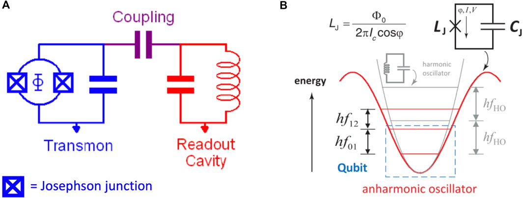
Figure 1. Basic scheme of a transmon. (A) The double J-J forms a loop with shunting capacity (blue), the read-out $LC$ resonator (which could be replaced by a resonant cavity), and the coupling capacity (grey). (B) Difference between the linearly spaced levels of the harmonic oscillator and the non-linearly spaced levels in the magnetically driven cosine potential.

3.2 Charge qubit

Starting from the three basic implementations, different and more advantageous types of SC qubits have been invented, the transmon being by far the most popular. Based on the charge-qubit model, in which the number of Cooper pairs $N$ is the main variable, a flux-tunable transmon can be realized with double J-J (a modified SQUID loop, first proposed by J. Koch’s group in 2007 (Koch et al. (2007); Figure 1A) that can store an energy $E_J=({\mathrm{\Phi }}_0/2\pi )I$. The circuit is shunted by a large coupling capacitance, such that the coupling energy $E_C=e^2/2C\ll E_J$, thus giving a large $Q$. The advantage of such a double-J-J is that the values of magnetic flux $\mathrm{\Phi }$ can be fine-tuned, and each qubit can be individually addressed by a “gate” (actually, a sequence of GHz pulses). The state of the qubit is read out by a second resonator (“cavity”) whose resonant frequency $f_R$ is chosen to be far from $f_{01}$. Then, the two possible qubit states show up as a (small) red- or blue-shift $\mathrm{\Delta }$ about the central read-out frequency, $f_R\pm \mathrm{\Delta }$.

The Hamiltonian of the classical equivalent circuit can be written as

$\mathcal{H}=4E_C{\left(N-\frac{1}{2}\right)}^2-E_J\cos \varphi +\underline{W\left(t\right)\sin \left({\mathrm{\Omega }}_{R}t+\varphi \right)}.(2)$

The quantum version for the transmon qubit (such as found in IBM Quantum System or Google Sycamore) runs on a slightly modified version of the celebrated Jaynes–Cummings theoretical model (Lo et al., 1998) and looks like

$\widehat{\mathcal{H}}=\hslash \sqrt{8E_C{E}_J}\left(a^{†}a+\frac{1}{2}\right)-\hslash E_C\left(a{\widehat{\sigma }}^{+}+a^{†}{\widehat{\sigma }}^{-}\right)+\underline{{\mathrm{\Omega }}_R\left[\mathcal{J}\left(t\right){\widehat{\sigma }}_x+\mathcal{Q}\left(t\right){\widehat{\sigma }}_y\right]}.(3)$

In the two equations, the underscored parts represent the external field (a train of microwave pulses) driving the Hamiltonian. $N$ is the number of excess Cooper pairs destroyed/created by the operators $a,a^{†}=\sqrt{n}|n\mp 1\rangle \langle n\pm 1|$; ${\widehat{\sigma }}_{x,y,z}$, and ${\widehat{\sigma }}^{\pm }={\widehat{\sigma }}_x\pm i{\widehat{\sigma }}_y$ are Pauli matrices; ${\mathrm{\Omega }}_R$ is the Rabi frequency; $\mathcal{J}$ and $\mathcal{Q}$ are the in-phase and quadrature components of the microwave signal $W(t)$. In principle, $N$ and $\varphi$ are both good quantum numbers to describe the transmon; however, in the $E_C\ll E_J$ limit, only $N$ is well-defined, while $\varphi$ fluctuates randomly.

3.3 Flux qubit

A variant of the transmon is realized with an SC ring interrupted by three or four Josephson junctions. The qubit is engineered so that a persistent current flows continuously when an external magnetic flux is applied. Notably, only an integer number of flux quanta can penetrate the SC ring, resulting in clockwise or counterclockwise mesoscopic supercurrents (typically 300 nA) in the loop, which compensate (screen or enhance) a non-integer external flux bias. The $\varphi$ degree of freedom becomes now the main variable, the number of flux quanta $N$ being random, and the coupling energy dominates over the charging energy, $E_J\ll E_C$.

When the applied flux through the loop is close to a half-integer number of flux quanta, the two lowest-energy loop eigenstates are found in a quantum superposition of the two currents. This is what makes the flux qubit a spin-1/2 system with separately tunable $z$ and $x$ fields.

The flux qubit has been used as a building block for quantum annealing applications based on the transverse Ising Hamiltonian (Hauke et al., 2020). A typical quantum Hamiltonian that can be implemented in a connected network of flux qubits, such as in the D-WAVE Chimera or Pegasus architectures, looks like

$\widehat{\mathcal{H}}=\mathrm{\Lambda }\left(t\right)\left[{\displaystyle \sum _i}{h}_i{\widehat{\sigma }}_i^z+{\displaystyle \sum _{i<j}}{J}_{ij}\left({\widehat{\sigma }}_i^z\cdot {\widehat{\sigma }}_j^z\right)\right]+\mathrm{\Gamma }\left(t\right){\displaystyle \sum _i}{\mathrm{\Delta }}_i{\widehat{\sigma }}_i^x.(4)$

The $h_i$ are asymmetry energies, $J_{ij}$ represent the coupling matrix elements, and ${\mathrm{\Delta }}_i$ are tunneling energies. At the beginning of the quantum annealing process, $\mathrm{\Gamma }(0)$ = 1 and $\mathrm{\Lambda }(0)$ = 0 create a known ground state as an equal superposition in the computational basis. During the adiabatic annealing protocol, the two parameters slowly evolve towards $\mathrm{\Gamma }\to 0$ and $\mathrm{\Lambda }\to 1$.

Other transmon variants have been proposed to counter some of the practical problems encountered in the different SC loop implementations, such as the C-shunt flux qubit (You et al., 2007), to reduce charge noise; the “fluxonium” (Manucharyan et al., 2009), to address the noise from inductance and offset charge; the “0-$\pi$” qubit (Brooks et al., 2013; Gyenis et al., 2021), designed to improve the symmetry of the two current states; and various types of hybrid qubits (see, e.g., Marcos et al. (2010); Kubo et al. (2010); Zhu et al. (2011)), in which the SC loops are coupled to solid-state elements, a doped crystal, or a resonant cavity, to exploit the advantages from different quantum effects. The key objective of increasing the lifetime of the qubit state has been pursued in recent years, extending the coherence time from mere fractions of $\mu$s well into the ms domain (Pop et al., 2014).

The next important operation to consider is the read-out of the information from the qubit. For solid-state qubits, this may be performed by energy-selective escape from a metastable potential (Martinis et al., 2002; Hanson et al., 2005) or with a bifurcation amplifier (Siddiqi et al., 2004; Mallet et al., 2009). For the SC loops, it is possible to detect either charge, flux, or inductance. A popular method is the dispersive read-out (Wallraff et al., 2004), in which the qubit and the resonator (see again Figure 1A) are coupled by a strength parameter $g\ll \mathrm{\Delta }={\omega }_{01}-{\omega }_R$, as in the approximate Hamiltonian:

$\widehat{\mathcal{H}}=-\frac{{\omega }_{01}}{2}{\widehat{\sigma }}^z+\left({\omega }_R+\frac{g^2}{\mathrm{\Delta }}{\widehat{\sigma }}^z\right)a^{†}a.(5)$

The presence of a $|0\rangle$ or $|1\rangle$ state in the qubit shows up as a small frequency shift in the resonator by the quantity $g^2/\mathrm{\Delta }$. The read-out is “dispersive” because the signal corresponding to the two possible states appears clustered in two disjointed clouds in the complex plane (Blais et al., 2021). The theory behind this technique has been established for systems both in and out of equilibrium and for general two-level-driven systems, non-Markovian dynamics, and thermally excited multilevel systems (Kohler (2017; 2018); Shen et al. (2022); Yang and Shen (2024)).

3.4 Qubits and quantum gates

Independently from their actual physical implementation, qubits are mathematically defined as two-state quantum systems, described by a state vector in a two-dimensional Hilbert space, spanning a closed surface with conserved norm (i.e., a sphere, called the “Bloch sphere,” Figure 2A). A standard basis is defined by the two vectors $|0\rangle$ and $|1\rangle$, conventionally aligned with the positive and negative direction of the z-axis.

Figure 2

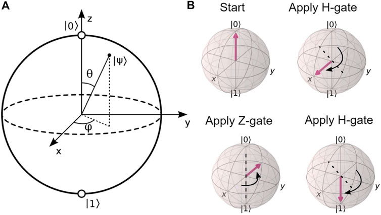
Figure 2. (A) The Bloch sphere. (B) Schematic of the transformation on the Bloch surface corresponding to the sequential application of a $H$, $Z$ and again a $H$ gate, resulting in the spin flip from $|0\rangle$ to $|1\rangle$ (and, therefore, equivalent to an $X$ gate).

A quantum computer executes a sequence of unitary transformations, $U_1\dots U_n$, as specified by a quantum algorithm, with each transformation acting on one or two (rarely three) qubits. The unitary transformation is executed by a “gate,” which is actually a physical operation that makes an external system (microwave or laser pulse, magnetic field switch, AC/DC signal) interact with the qubit to modify its state. For a single qubit it is often a rather simple operation, such as a microwave pulse at the exact frequency of the J-J junction. For two-qubit gates it may be more complicated because qubits are, in principle, arranged in such a way that they do not interact with each other in their ground state. Coupling can be realized, for example, by properly designing the capacitance between the pair (Yamamoto et al., 2003), through their mutual inductance (Hime et al., 2006), by a microwave cavity in which confined photons transfer the quantum state between qubits (Majer et al., 2007), or yet by other means.

One-qubit gates act on either the phase or the excitation energy of a single qubit by applying a rotation on the Bloch surface (Figure 2B). The states of the qubit can be represented as column vectors, $|{\psi }_1\rangle =\left(\begin{array}{c}1\\ 0\end{array}\right)$ and $|{\psi }_2\rangle =\left(\begin{array}{c}0\\ 1\end{array}\right)$. Then, the simplest operations of transformation of the state (a “gate”) can be schematized by $2\times 2$ matrices. An arbitrary rotation of the qubit state about an axis $\widehat{\mathbf{n}}$ is represented as $U_{\widehat{\mathbf{n}}}(\varphi )=\exp (-i\varphi \widehat{\mathbf{n}}\cdot \vec{\sigma })=\cos (\varphi )\mathbf{I}-i\sin (\varphi )(\widehat{\mathbf{n}}\cdot \vec{\sigma })$, with $\vec{\sigma }$ being the block vector that has the Pauli matrices as its xyz components.

In the case of the transmon, standard rotation gates are available (hardware implemented) in the xy plane or in the z axis. For the xy single-qubit gate, the Hamiltonian reads

$\mathcal{H}=-\frac{\hslash }{2}{\omega }_{01}{\sigma }_z+W\cos \left({\omega }_{R}t-\varphi \right){\sigma }_x=-\frac{\hslash }{2}\left[\mathrm{\Delta }{\sigma }_z-W\left(\cos \varphi {\sigma }_x+i\sin \varphi {\sigma }_y\right)\right].(6)$

When the microwave (MW) frequency is exactly tuned to the qubit frequency, $\mathrm{\Delta }$ = 0, and the rotation in the xy plane is fixed only by the choice of the phase angle $\varphi$. This makes the $xy$ or phase gate one of the most important elements of quantum computing.

Students may find it difficult to grasp the meaning of the phase gate because, in introductory quantum mechanics classes, the role of the phase remains rather obscure and is often swept under the carpet by noticing that “phase disappears when taking the $|\psi {|}^2$ of the wavefunction.”³ If the output of a measurement is a random distribution, one can only accumulate probability amplitudes of each instance in a classical setting; however, in the quantum calculation, constructive or destructive interference allows amplifying or suppressing some of the outputs by manipulating the phases of the qubits. A great example is the quantum Fourier transform (QFT), which finds periodic instances in a sequence, like its classical counterpart. The QFT algorithm transforms a $m$-bit state $|\psi \rangle ={\sum }_i{\alpha }_i|i\rangle$ to $|{\psi }^{\prime }\rangle ={\sum }_i{\beta }_i|i\rangle ={\sum }_i{\sum }_k{\alpha }_i{e}^{2\pi i{\varphi }_k}|i\rangle$, $i,k=1\dots m$. It requires the application of one Hadamard gate to each pair of qubits, followed by a sequence of phase gates for each term in the $k$-sum, resulting in a total of $m$ Hadamard + $m(m+1)/2$ phase gates (that is, $\mathcal{O}(m^2)$ polynomial complexity).

Two-qubit gates carry out controlled transformations of the second qubit state (target), conditioned by the state of the first one (control). Compared to single-qubit gates, whose working speed is limited by the strength of the driving fields (Frey, 2016), two-qubit gates (notably, the entangling gate) can only operate at a speed proportional to the interaction strength between the qubits (Steane et al., 2014; Schäfer et al., 2018). This is typically weaker than available single-qubit drive strengths and cannot be easily increased, thereby representing one important limit to the coherence time (see below). For the SC qubits, moreover, the limited anharmonicity makes single-qubit gates not much faster than two-qubit gates (Stehlik et al., 2021; Moskalenko et al., 2022).

As the two-qubit state is a column vector of dimension 4, the gates can be written as a 4 × 4 matrix. The controlled transformations can be of two main types: the Controlled-NOT (CNOT), which leaves $|00\rangle$ and $|01\rangle$ unaltered and swaps $|10\rangle$ and $|11\rangle$; and the Controlled-Phase (CPHASE), which flips the phase of the two-qubit state if both the qubits are excited. It is interesting to note that CNOT can be constructed by applying Hadamard to the target qubit, then CPHASE to this new state, and Hadamard again (see, e.g., Wallquist et al., 2005). The ensemble of a CNOT gate, the Hadamard, and all phase gates form an infinite set of universal gates, by which any $m$-qubit unitary operation can be represented using $\mathcal{O}(m{4}^m)$ such gates.

3.5 Entanglement

It is worth noting once more that coupling is not the same thing as entanglement. Coupling refers to the physical mechanism allowing the exchange of information between different qubits. The result can be either a non-entangled, a partially entangled, or a maximally entangled state vector $|\psi \rangle$ (Franco and Compagno, 2016). If ${\rho }^2$ = $\rho$, with $\rho$ = $|\psi \rangle \langle \psi |$, the state is pure by definition. To check if it is also entangled, however, we may look at the purity of the respective substates describing its parts. Imagine a system divided into two parts with coordinates $q_1,q_2$, and in a pure state $|{\psi }_{12}\rangle =|\psi (q_1,q_2)\rangle$ such that ${\rho }_{12}=|{\psi }_{12}\rangle \langle {\psi }_{12}|$; each subsystem lives in a state described by the reduced density ${\rho }_1={\mathrm{Tr}}_2\{{\rho }_{12}\},{\rho }_2={\mathrm{Tr}}_1\{{\rho }_{12}\}$. Then, if the state wavefunction is not factorizable into pure states for 1 and 2, $|{\psi }_{12}\rangle \ne |{\psi }_1\rangle \otimes |{\psi }_2\rangle$, the two subsystems are entangled, and their respective reduced density describes a mixed state for each part (Caban et al., 2015). When a state is written out as a sum of basis vectors, determining whether it is separable is not always obvious. For example, a general two-qubit pure state like $|\psi \rangle =a|00\rangle +b|01\rangle +c|10\rangle +d|11\rangle$ is separable when $a$ = $b$ = $c$ = $d$, as $|\psi \rangle =a(|0\rangle +|1\rangle )(|0\rangle +|1\rangle )$. however, it is not separable (entangled) for $b$ = $c$ = 0 because both qubits are now in a mixture of $|0\rangle$ and $|1\rangle$.

The differences here are subtle and worth explaining. Separable states can be written as a combination of product states; product states, in turn, can be written as direct product $\otimes$ of quantum states living in each subspace. Product states have no correlation at all among the degrees of freedom of the subspaces, whereas separable states can have correlations, which, however, are entirely classical. Entangled states have a higher degree of correlation of purely quantum origin.

Maximally entangled states are called “Bell states.” The meaning of maximum entanglement is usually taken as the maximization of von Neumann’s entropy (see below, Eq. 27 and on). A simpler interpretation is that the state is described by a single wavefunction (i.e., not separable) so that a measurement of any qubit gives the values of all the others deterministically. (In contrast, a mixed state would give a statistical mixture of all qubits.)

Entangled states can be obtained by the sequential application of a Hadamard single-qubit gate, followed by a CNOT. The Hadamard produces a 50/50 superposition of the basis states, for example,

$\left[H\right]|0\rangle =\frac{1}{\sqrt{2}}\left(\begin{array}{cc}\hfill 1\hfill & \hfill 1\hfill \\ \hfill 1\hfill & \hfill -1\hfill \end{array}\right)\left(\begin{array}{c}\hfill 1\hfill \\ \hfill 0\hfill \end{array}\right)=\frac{1}{\sqrt{2}}\left(\begin{array}{c}\hfill 1\hfill \\ \hfill 1\hfill \end{array}\right)=\frac{|0\rangle +|1\rangle }{\sqrt{2}}.(7)$

Then, the CNOT gate operates on the product states, such as $|{\psi }_p^{\pm }\rangle =\frac{1}{\sqrt{2}}(|0\rangle \pm |1\rangle )\otimes |p\rangle$, $p=\mathrm{0,1}$ to obtain the finally entangled states. For example,

$\left[CNOT\right]|{\psi }_0^{+}\rangle =\frac{1}{\sqrt{2}}\left(\begin{array}{cccc}\hfill 1\hfill & \hfill 0\hfill & \hfill 0\hfill & \hfill 0\hfill \\ \hfill 0\hfill & \hfill 1\hfill & \hfill 0\hfill & \hfill 0\hfill \\ \hfill 0\hfill & \hfill 0\hfill & \hfill 0\hfill & \hfill 1\hfill \\ \hfill 0\hfill & \hfill 0\hfill & \hfill 1\hfill & \hfill 0\hfill \end{array}\right)\left(\begin{array}{c}\hfill 1\hfill \\ \hfill 0\hfill \\ \hfill 1\hfill \\ \hfill 0\hfill \end{array}\right)=\frac{1}{\sqrt{2}}\left(\begin{array}{c}\hfill 1\hfill \\ \hfill 0\hfill \\ \hfill 0\hfill \\ \hfill 1\hfill \end{array}\right)=\frac{1}{\sqrt{2}}\left(|00\rangle +|11\rangle \right).(8)$

For two qubits, the four possible Bell states obtained by combining all product states are given by

$\begin{array}{cc}\hfill & |{\psi }_B^{\pm }\rangle =\frac{1}{\sqrt{2}}\left(|00\rangle \pm |11\rangle \right)\hfill \\ \hfill \\ \hfill & |{\varphi }_B^{\pm }\rangle =\frac{1}{\sqrt{2}}\left(|01\rangle \pm |10\rangle \right)\hfill \end{array}.(9)$

However, not all entangled states are Bell states. For example, the states $|\psi \rangle =\cos (\theta )|00\rangle +\sin (\theta )|11\rangle$ for $\theta \in (0,\pi /4)$ are all entangled but are not Bell states.

A last point worth noting is that the time profile of the interaction Hamiltonian is controlled by classical parameters, such as the intensity of a laser beam, the value of the gate voltage, or the current intensity in a wire. Of course, all such parameters are also quantum mechanical in nature when examined at the atomic level; the fact that they behave classically means that there should be no entanglement between their (very large) quantum states and the internal states of the qubits of the quantum computer.

3.6 Decoherence, dephasing, thermalization

All physical quantum systems are subject to decoherence and dissipation, mainly arising from their noisy interaction with the environment. As we will see later (Section 5), when exploring the connection between thermodynamics and information, any realistic sequence of operations of a quantum information processing device is irreversibly accompanied by the production of entropy, which pairs with the irretrievable loss of (quantum) information into the environment. Then, some questions immediately appear:

$•$ What are the physical limitations on information processing set by thermodynamics?

$•$ Can we maintain quantum computers in the deep quantum regime so that we can actually exploit their advantage w/r to classical computers?

$•$ The exponential increase in computing capability will entail an exponential increase in thermodynamic work and dissipated heat?

Within a standard picture for spin-1/2 systems, two characteristic decay rates contribute to coherence loss: ${\mathrm{\Gamma }}_1=1/T_1$ is the longitudinal relaxation rate (an energy decay rate), which is the time over which the qubit exchanges energy with its environment; ${\mathrm{\Gamma }}_2=1/T_2=1/(2T_1+1/T_{\varphi })$ is the transverse relaxation rate (a decoherence rate), which is the time over which the device remains phase-coherent. In simpler words, $T_1$ is the time taken by a qubit to decay spontaneously, for example, from $|1\rangle$ to $|0\rangle$, while $T_2$ is where a qubit dephases into a mixture of states such that the phase can no longer be accurately predicted. Over the past 20 years, a steady increase in $T_2$ has brought superconducting qubits from the stage of laboratory experiments to the capability of building the first quantum computers (Oliver and Welander, 2013; Gil and Green, 2020).

Currently, the error rate on the best quantum computers is approximately 1% for each elementary operation. Although a 99% accuracy may seem already high, a single mistake affects the whole entangled system: even one error corrupts the result. One way to improve errors could be to replicate $N$ identical copies of the logical unit and have them “vote” on the output. Only if all $N$ physical qubits give the same answer is the logical qubit considered correct. (This is similar to what happens in classical computers, for example, with the Hamming correction code.)

Another method that is becoming standard is the introduction of correction, or “ancilla,” qubits, with the same logic as the parity bit in classical digital computers. The ancilla qubit is prepared in $|0\rangle$, and then a sequence of CNOT gates is applied from the working qubits onto the ancilla qubit. These gates flip the ancilla or “check bit” between $|0\rangle$ and $|1\rangle$ an even or odd number of times, depending on the parity of the bit string stored in the data qubits. When the ancilla qubit is measured, the parity of the state is the only thing that is measured without interfering with the rest of the quantum computation.

However, as the number of logical qubits grows, the number of layers to correct the original plus the correction qubits grows exponentially. Google’s Labs' estimate is that current technology may require 1,000 physical qubits to encode one logical qubit and attain an error rate of one in $10^9$.

Introduced as a measure of the practical estimate of the minimal availability of quantum resources to perform a computation, the quantum volume of a quantum computer depends on the number of qubits $N$, as well as the number of steps that can be executed while remaining in a coherent state, that is, the circuit depth, $d$:

$V_Q=\min {\left[N,d\left(N\right)\right]}^2.(10)$

The variation of $d$ with the number of qubits is $d(N)\simeq 1/(Nϵ)$ for an average error rate $ϵ$. However, a quantum algorithm typically engages subsets of $n$ qubits from those available in the whole machine $N$. IBM’s modified definition of quantum volume (Moll et al., 2018) is the equivalent complexity to simulate the same quantum circuit on a classical computer:

${\log }_2{V}_Q=\underset{n\le N}{\max }\left\{\min {\left[n,d\left(n\right)\right]}^2\right\}.(11)$

Such definitions only provide a measure of the theoretical feasibility of a computation, neglecting other constraint factors such as read-out times, 1/$f$ noise, quantum error correction, and magnetic or current (phase) fluctuations.

4 Thermodynamics in a classical digital computer

Thermodynamics was developed in the nineteenth century to provide a unified framework between mechanical sciences and calorimetry. At the time, the motivation was very practical, namely, the use of temperature differences to generate heat that could put bodies into motion—as clearly indicated by its name, thermo (heat) and dynamo (movement). In other words, the goal was to design and optimize thermal engines, that is, devices that exploit the transformations of some “working substance” between different temperatures to convert heat into work. Work and heat are two ways to exchange energy; according to the first law of thermodynamics, it is possible to convert one into another.

However, turning heat into work and back into heat comes at a cost: it is not possible to cyclically extract work from a single hot bath (Kelvin, 1851), and while any amount of work can generate the same amount of heat, heat can never be converted into the same amount of work⁴. This no-go statement is one of the expressions of the second law of thermodynamics, which ultimately deals with irreversibility. Interestingly, the concept of work came originally from mechanical sciences (Lazare Carnot, 1803) and represents a form of energy that can be exchanged reversibly: in principle, there is no time arrow associated with work exchanges (at least for conservative forces) because the equations of motion in classical mechanics are perfectly time-reversible. When building steam machines, it is always found that heat $Q$ spontaneously flows (only) from hot to cold bodies. To extract work $W$, a source and a sink at different temperatures $T_1$ and $T_2$ are necessary, independently of the nature of the exchange medium, as stated by Sadi Carnot in 1823 in an idealized experiment, the “Carnot cycle,” for which he derived a theorem regarding the efficiency of a machine producing work.

A Carnot cycle is a closed ensemble of operations by which a thermodynamic machine starts from a condition and returns to the same condition after having performed some work at the expense of the heat extracted from a source at a higher temperature than a sink. The theorem states that the ideally reversible engine produces work from heat if and only if the sink temperature is lower than the source temperature, $T_2<T_1$. If $T_2>T_1$, work must be supplied to the engine. If, on the other hand, $T_1=T_2$, no work can be extracted. The Carnot cycle can be run in the “forward” direction and “in reverse” because it is, in theory, fully reversible and designed to have the maximum possible thermodynamic efficiency. When running in the opposite direction, the same amount of work performed in the forward cycle is returned to the source as heat; the sum of the forward and reverse operations results in zero net energy consumed and zero network extracted. All such considerations, however, remain in the domain of idealized systems. The practical problem with such an ideal situation is that the heat is extracted from the source and transferred to the sink while remaining at constant temperature, $T_1$ and $T_2$, apparently contradicting the experimental observation that $Q$ only flows from hot to cold bodies. Furthermore, to move from $T_1$ to $T_2$ and back, a rigorously lossless transformation is required, which in practical terms means proceeding at an infinitely slow rate.

4.1 Entropy is the name we give to our losses (Clausius, 1856)

The second law of thermodynamics is quite different from other laws in physics because (i) there are many different statements for the same law, and (ii) it is only a qualitative description rather than a quantitative relationship between physical quantities. Clausius wanted to put Carnot’s theorem on a more general basis, considering that heat exchanges between a body and a thermal bath are not always reversible in the real world and imply a loss of energy to the environment. He introduced the notion of entropy, $S$, as the ratio between heat exchanged and working temperature, encompassing both reversible and irreversible transformations in the single inequality:

$Q\left(\frac{1}{T_{\mathit{low}}}-\frac{1}{T_{\mathit{high}}}\right)=\mathrm{\Delta }S\ge 0.(12)$

Hence, it is usually said that the second law of thermodynamics introduces the notion of a time arrow. Here, we already could start thinking of the analogy with the operations being carried out in a digital computer, accompanied by a waste of heat. The computer is, in principle, maintained at constant temperature; however, it is an engine consuming energy to perform a computation, and its temperature increases (in the absence of refrigeration and heat removal) at each operation performed. This energy goes into the flow of electrons that move around the integrated circuits, capacitors, resistances, and connecting wires. We can use Maxwell equations to deduce the amount of power accompanying the current. However, the fundamental operations that the computer is doing are creating and destroying information by using this electrical current to flip the bit states in its memory from 0 to one and vice versa. Is there a link between the logical operations of creating and destroying information and the energy required to physically run the computing machine?

4.2 Statistical definition of entropy (Boltzmann 1875)

In order to make such a link, we must at least be able to find a connection between the macroscopic world of thermodynamics and the microscopic world in which electrons move and collide with other electrons and lattice vibrations (phonons). The connection between the macroscopic and microscopic degrees of freedom was attempted by Boltzmann by introducing the notion of microstate, which is a definition of the instantaneous condition of the microscopic degrees of freedom (i.e., positions and momenta) that make up a macroscopically observable state. As it is immediately evident, a macroscopic state can be obtained in a variety of microscopic ways: the air molecules in a room continuously change their microstate while the overall temperature and pressure remain constant.

Boltzmann introduced the following microscopic expression for the entropy, interpreted as an extensive function that “counts” the number of microstates of the system:

$S=k_B\ln \mathrm{\Omega }.(13)$

$\mathrm{\Omega }$ is the number of microscopic states compatible with a given set of thermodynamic constraints $(T,P,V,N,\dots )$. $\mathrm{\Omega }$ is a very difficult quantity to compute or even to estimate, except in some very simple cases, such as the perfect gas:

$\mathrm{\Omega }=\frac{1}{N!}{\left(2mE\right)}^{3N/2}{V}^N.(14)$

This statement is valid in the “microcanonical” statistical mechanics ensemble at constant $\{N,V,E\}$. For this experimental setup, all microstates are equiprobable at equilibrium.

In contrast, for constant $\{N,V,T\}$ conditions, that is, the “canonical” ensemble, microstates are not equiprobable but are distributed according to the Boltzmann probability $\exp (-E/k_{B}T)$, and the energy $E$ is replaced by $k_{B}T$ in the definition of $\mathrm{\Omega }$, because $T$ is now constant and all energy values $E$ are allowed. That is, energy can fluctuate. Fluctuating quantities are not usually considered in macroscopic thermodynamics, which deals only with average values at equilibrium. Macroscopically, we expect a system to have both a well-defined temperature and well-defined energy. However, when we look at the microscopic scale, for a given temperature, the energy can fluctuate between different values. The macroscopic condition is recovered because energy fluctuations $\mathrm{\Delta }E$ are proportional to the (square root of) specific heat, an intensive quantity proportional to the number of degrees of freedom $N$ of the system:

${\left(\mathrm{\Delta }E\right)}^2=k_B{T}^{2}N{c}_V.(15)$

Hence, when we calculate the relative importance of energy fluctuations with respect to the absolute value of the intensive quantity energy, it is $\mathrm{\Delta }E/E\propto \sqrt{N}/N=1/\sqrt{N}$. In other words, in the limit of a macroscopic system $N\sim 10^{24}$, the energy is practically constant. Equation 15 is an example of a fluctuation–dissipation relation, establishing a relationship between the thermal fluctuations of a physical quantity (energy) and another quantity (the specific heat) that describes its dissipation.

4.3 CMOS power dissipation: how big is a bit?

Logical units in digital computers are made by combining a number of transistors carved with high density in the silicon chip. When the transistor is in a given logical state, its current consumption is negligible. All of the energy dissipation takes place during transitions between logical states, and the source of this dissipation is the need to charge or discharge the related capacitors. The energy dissipated to charge/discharge one CMOS transistor has a well-established form:

$E_{\mathit{switch}}\simeq \alpha C_{\mathit{node}}{V}^2\simeq 0.01\cdot 10^{-12}\cdot {\left(3\right)}^2\simeq 0.1\text{\hspace{0.17em}pJ}\simeq \mathcal{O}\left(10^7\right)k_{B}T(16)$

for a supply voltage of 3 V, $C_{\mathit{node}}$ is the lumped capacitance, and $\alpha$ is a coefficient that includes the clock frequency (Wiltgen et al., 2013). In the Xeon Broadwell-E5 (14-nm technology), approximately 7.2 million transistors arranged in approximately one million logic gates (making up CPU, memories, controllers, etc.) are packed in 456 ${\text{mm}}^2$. Therefore, each transistor covers approximately $8\times 8$ $\mu {\text{m}}^2$, with a thickness of $\sim$0.2 mm, that is approximately 150 billion Si atoms. So each atom dissipates approximately $10^{-4}{k}_{B}T$ at each switching of the transistor.

However, switching is a collective, statistically uncorrelated process: atoms follow quantum mechanics; currents follow Maxwell’s equations. A question arises: is there a link between the heat dissipation and the use/transfer/loss of information?

4.4 Thermal noise and random bit flips

The flow of electrons in any current-conducting medium, for example, across a resistor, is affected by thermal fluctuations that entail a voltage fluctuation, with a spectrum usually assumed to be Gaussian with zero mean. The Johnson–Nyquist formula (originally derived on the basis of the equipartition law (Johnson, 1928; Nyquist, 1928)) gives the thermal noise power density as the product of thermal energy by the bandwidth, $P=k_{B}T\mathrm{\Delta }f$. To fix a number, a 1 kOhm resistor at room temperature with a bandwidth of 1 Hz generates a root mean square (RMS) noise of 4 nV. Although a capacitor is ideally a noiseless device, when combined with resistors, it generates noise. Because $\mathrm{\Delta }f$ is inversely proportional to $\sqrt{RC}$ and given the steady reduction of the oxide layer with increasing transistor density, the overall result of CMOS miniaturization is an increase in the RMS width of the Gaussian voltage noise.

Under such conditions, there is a finite probability that a spike in the voltage noise $V_n$ could pass, every now and then, the threshold voltage $V_{th}$ to flip the bit, in a random fluctuation. The average frequency by which such an event can occur can be estimated from the Rice formula (Rice, 1945), whose result in the approximation of white noise is

$\nu ={\nu }_0\exp \left(-\frac{V_{th}^2}{2V_n^2}\right).(17)$

Due to the steep dependence on the square of the $V_{th}/V_n$ ratio, the frequency of a random bit-flip is estimated approximately 35 million per hour at $V_{th}/V_n\simeq 5$ and drops to 2 in $10^{-9}$ per hour (that is, approximately 20 errors per hour in a 1-Gbyte RAM chip) at $V_{th}/V_n\simeq 10$ (Kish, 2002). In recent years, the threshold voltage $V_{th}$ has been constantly reduced, proportional to the decrease in supply voltage, and in the most advanced CMOS circuits, it could be of the order of $\sim$0.45 V. Requiring the signal/noise voltage ratio to be at least $>$10 implies that the RMS thermal voltage fluctuation must be kept below approximately 35 mV to ensure a safe operation or a maximum temperature of $T=e{V}_n/k_B\lesssim 150^o$C. Because leakage currents start affecting silicon electronics above $\sim 180^o$C, random bit flipping is likely the main thermal limit to further decrease of voltage, the peak temperature of hot-spots in dense multiprocessor arrays being in the $\sim {100-120}^o$C (normal electronics are rated to function to ${85}^o$C, and military electronics are rated to ${125}^o$C, which actually seems a bit of a stretch, in view of the rapidly increasing bit-error rate).

5 Information and thermodynamics: the demons of Leo Szilard

5.1 Information is physical (Landauer, 1961)

One important achievement in the study of information processing has been making the link with thermodynamics, with the understanding that manipulating information is inevitably accompanied by a certain minimum amount of heat generation. Computing, like all processes proceeding at a finite rate, must involve some dissipation. More fundamentally, there is a minimum heat generation per operation, independent of the actual rate of the process. The binary logic devices of digital computers must have at least one degree of freedom associated with the information they carry. Typically, a logic port with more than one input, and only one output mixes information from the input data to present a value to the single degree of freedom of its output. As we will see below, devices with more input ports than output ports are inherently irreversible in that the output does not allow reconstruction of the input information. Such devices exhibiting logical irreversibility are essential to classical computing. The important point is that logical irreversibility implies physical irreversibility, which is accompanied by dissipative effects. The Boltzmann expression, such as Eq. 13, makes a link between entropy and the number of microstates available for a system at a given energy, showing that the larger is $\mathrm{\Omega }$, the larger the distribution of possible configurations (in quantum terms, we could think of some analogy with mixed states). The dynamical equations, perfectly reversible at the level of individual degrees of freedom, become practically irreversible when the number of degrees of freedom gets very large. If we film two colliding balls and play the movie in reverse, it is impossible to tell the past from the future. If, however, we film a single ball hitting a triangle at snooker and play the same trick, it is immediately evident that the future is the one with more disorder at the end: the larger $\mathrm{\Omega }$ brings more entropy and less information about the dynamics of the individual trajectories. For a snooker game with Avogadro’s number of balls, the information about past physical trajectories is irreversibly lost.

Rather than counting microstates à la Boltzmann, entropy can also be rewritten (Gibbs, Jaynes (1965)) in terms of the absolute probability of each microstate:

$S=-k_B{\displaystyle \sum _i}{p}_i\ln p_i.(18)$

For the microcanonical ensemble in which all the $p_i=1/\mathrm{\Omega }$, this writing is exactly the same as Boltzmann’s Eq. 13 (which was actually put down in that form by Max Planck). For a distribution $p_i=\exp (-E_i/k_{B}T)$, instead, it easily shown that the canonical ensemble is obtained with constant $N,V$ and $T$ (Goldstein et al. (2020)).

The notion of information entropy was defined by Shannon (1948) when he tried to quantify the “loss of information:”

$H=-{\displaystyle \sum _i}{p}_i\ln p_i.(19)$

It can be viewed as the entropy change due to the presence/absence of information about a system, and it actually was von Neumann who suggested to Shannon the evident equivalence between his definition and Boltzmann’s statistical mechanics formulation. However, pushing the analogy even further forward, could it also be a measure of a heat loss accompanying the exchange of information?

5.2 The Szilard engine, 1929

Instead of considering a gas made of many particles (Carnot), consider only one single particle that is either on the left or on the right of a chamber equipped with two frictionless “pistons” and a “wall.” “Left” or “right” positions can be used to encode 1 bit of information (Figure 3). A “demon” who knows in which side of the box the particle is at time t = 0 can spend this information (entropy) to:

1. close the wall between the two halves of the box; then

2. let the piston in the empty side move by doing zero work until it reaches the closing wall; and finally

3. extract useful work by opening the wall and leaving the particle to expand back (isothermally) to its original equilibrium volume.

Figure 3

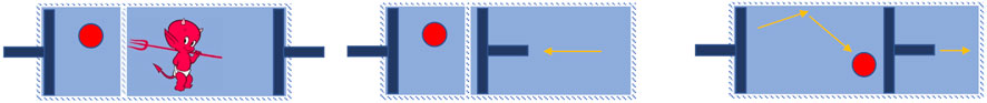
Figure 3. The Szilard engine and its demon.

This thought experiment was designed by Szilard (1929) to prove that possessing and using pure information has measurable thermodynamic consequences. Denoting by $p$ the probability that the particle is (for example) found on the left, the Shannon entropy for the 1-particle engine reads

$H\left[p\right]=-p\ln p-\left(1-p\right)\ln \left(1-p\right).(20)$

If the demon has zero information, then: $p=(1-p)=1/2$, and $H[p]=-\ln 1/2=\ln 2$. However, if the demon has this 1 bit of information, $H$ must go to 0 upon completing the cycle and

$\mathrm{\Delta }H=H_{\mathit{fin}}-H_{in}=-\ln 2(21)$

Using the single bit of information thus corresponds to a reduction in the entropy of the system. The global system entropy is not decreased, but information-to-free-energy conversion is possible. After the particle is confined in one side of the box, the system is no longer in equilibrium: it appears that using information changed the system state without apparently changing the energy. Notably, the Szilard engine has been recently realized experimentally using Brownian particles (Toyabe et al., 2010) or single electrons (Koski et al., 2014).

(To be fair, the demon should have indeed more than 1 bit of information: he must first decide at what place to put the wall and then control the piston’s direction of motion. Therefore, at least three bits of information are required.)

Let us then consider a “computer” with $N$ binary bits. In the initial (prepared) all-zero state, all the $p_i=1$ and

$H_{in}=-N\ln 1=0.(22)$

After thermal equilibration, each bit has equal probability $p_i=1/2$ of being found in the state 0 or 1. This is to say that the initial information can be dispersed in any of the $N$ states, and the information entropy is

$H_{\mathit{fin}}=N\ln 2.(23)$

When we restore the initial state (that is, flush all voltages to ground and reset all bits to 0), a minimum heat of

$\mathrm{\Delta }Q=k_{B}T\mathrm{\Delta }H=k_{B}TN\ln 2(24)$

is wasted. The RESET operation (erasure) is irreversible, and the wasted information turns to heat. The huge difference between the theoretical $\ln 2$ and the $\mathcal{O}(10^9)k_{B}T$ observed for the heat dissipation of a real transistor is due to the accessory circuits and wiring around each bit of information, but the lower limit of $\ln 2$ is incompressible.

To check this absolute limit, imagine that our computer goes instead into a defined final configuration, in which some bits have a higher probability of being in a given state, as could be in the result of some calculation. For example, $N/2$ have $p=3/4$ and $N/2$ have $p=1/4$ of being in state 1 (and all have $1-p$ probability of being in 0):

$H_{\mathit{fin}}=\mathrm{\Delta }H=-\frac{N}{2}\ln \frac{3}{4}-\frac{N}{2}\ln \frac{1}{4}=N\left(\ln 4-\ln 3^{1/2}\right)>N\ln 2.(25)$

It is easily shown that any choice of $p_i$ different from $1/N$ gives a larger entropy. The value of $\ln 2$ appears, therefore, as an absolute lower bound for the heat dissipated by an operation destroying the information of a single bit.

For quantum systems, the statistical state is described by the density matrix $\rho$. The probability of having a certain state $|n\rangle$ out of a complete basis, as the outcome of a measurement, is $p_n=\langle n|\rho |n\rangle$. Therefore, the (Shannon) information entropy for such a measurement is

$S\left(\rho \right)={\displaystyle \sum _n}\langle n|\rho |n\rangle \ln \left(\langle n|\rho |n\rangle \right)(26)$

By changing to the basis in which the density matrix is diagonal, the entropy assumes its minimum value and is called the von Neumann entropy:

$S_{VN}\left(\rho \right)=-\mathrm{Tr}\left\{\rho \ln \rho \right\}(27)$

usually multiplied by the constant $k_B$ to give the entropy energy-like units. Evidently, the von Neumann entropy can be identified with the information entropy only if we pretend to know beforehand in which basis $\rho$ is diagonal. For an equilibrium state with Hamiltonian $\mathcal{H}$, this is the canonical state, $\rho =\exp (-\beta \mathcal{H})$. A rigorous definition of entropy, however, should not assume any special a priori basis. At least the (classical) uncertainty of the macroscopic measurement apparatus should be included, the quantum state entropy being written as a conditional probability $S(\rho |\mathcal{A})$ of obtaining a certain measurement outcome for a given measurement condition and averaged over all the measurable results $\mathcal{A}$ (Stotland et al., 2004):

${⟨S\left(\rho |\mathcal{A}\right)⟩}_{\mathcal{A}}=S\left(\mathcal{A}\right)+{\displaystyle \sum _{\mathcal{A}}}P\left(\mathcal{A}\right)S\left(\rho |\mathcal{A}\right),(28)$

where ${⟨\dots ⟩}_{\mathcal{A}}$ indicates ensemble averaging, $P(\mathcal{A})$ is the probability of finding the macroscopic measurement apparatus in the condition $\mathcal{A}$, and $S(\mathcal{A})$ is the corresponding classical entropy.

5.3 Landauer’s principle (classical)

Logical irreversibility is the act of processing information in which the output does not uniquely permit retrieving the inputs. Now, the link between Gibbs’ and Shannon’s definitions of entropy is a purely mathematical one: by dealing with two very different situations, different variables, and different processes, they arrive at two definitions of a measurable quantity that formally read identically. A plausible deduction is that these should be, therefore, the same quantity. Landauer (1961) and later Bennett (1982) tried to put the equivalence on more physical grounds. Their idea was that information at its most basic stage is a distribution of 0s and 1s physically entrusted to a set of bistable systems described by a bistable potential; then, the (classical) thermodynamics of each two-state system automatically associates the processing of information with the thermodynamics laws that those physical systems ought to follow. As a result, Shannon’s, Gibbs’, and Clausius’ entropies must describe the same thing, and logical irreversibility must imply thermodynamic irreversibility in the sense of the second law, that is, an increase of entropy (Ladyman et al., 2007).

The only nontrivial reversible operation a classical computer can perform on a single bit is the NOT operation, with one input and one output whose values are strictly defined. In contrast, the operations AND, NAND, OR, and XOR are all irreversible because they have more than one input and only one output. Hence, from the output of these logic gates, we cannot reconstruct the input: information is irreversibly lost. However, in a quantum computer, irreversible operations may be—at least ideally—avoided, for example, by saving the entire history of the process or by replacing the irreversible gates with more complex but reversible gates, for example, using a Toffoli gate instead of the AND. It seemed, therefore, that information processing at the quantum level should have no intrinsic thermodynamic cost, as first Bennett (1982) and then Feynman (1985) observed.

The operation of erasing a bit of information, instead, has two possible states (0 or 1) being mapped to a single definite state of 0, so it must entail a loss of entropy because the value 0 has now $p$ = 1, for both a classical and a quantum computer. A reformulation of the second law, Landauer’s principle states that the entropy decrease of the information-carrying degrees of freedom must always be compensated by an equal (or greater) entropy increase in the environment. Classical experiments in which the minimum heat dissipated to erase the initial state, with a colloidal particle optically trapped in a double well representing the two memory states, beautifully confirmed the link between information theory and thermodynamics (Bèrut et al., 2011).

5.4 Quantum computation is microscopically reversible

Qubits are defined as two-state quantum systems, described by a state vector in a two-dimensional Hilbert space, spanning a closed surface with conserved norm (i.e., the Bloch sphere). A standard basis is defined by two vectors $|0\rangle$ and $|1\rangle$, conventionally aligned with the positive and negative direction of the z-axis.

In principle, a quantum gate performs rotations in the Bloch sphere of one or more qubits onto which it is applied. Therefore, any quantum gate is a unitary operator:

$U{U}^{†}=U^{†}U=\mathbf{I}.(29)$

I is the identity operator. Such an operation conserves the norm of the quantum state and is perfectly time-reversible (Bennett, 1982; Feynman, 1985). Upon application of any sequence of quantum gates, state vectors span the whole surface of the Bloch sphere. Being unitary, qubit rotations (in principle) do not generate any heat.

A pure quantum state is one that cannot be written as a probabilistic mixture of other quantum states. Pure states can also result from the superposition of other pure quantum states (entanglement). A density matrix, $\rho =|\psi \rangle \langle \psi |$, can be used to represent both pure $({\rho }^2=\rho )$ and mixed $({\rho }^2\ne \rho )$ states. Let us look, for example, at two states in the 2-dim Hilbert space of a qubit, $|{\psi }_1\rangle =\left(\begin{array}{c}1\\ 0\end{array}\right)$ and $|{\psi }_2\rangle =\left(\begin{array}{c}0\\ 1\end{array}\right)$. Then, for a mixed state with equal probabilities $p_i=\frac{1}{2}$, we have

$\rho ={\displaystyle \sum _i}{p}_i|{\psi }_i\rangle \langle {\psi }_i|=\frac{1}{2}\left(\begin{array}{cc}\hfill 1\hfill & \hfill 0\hfill \\ \hfill 0\hfill & \hfill 1\hfill \end{array}\right).(30)$

On the other hand, for a pure state with equal amplitudes, $|\psi \rangle =\frac{1}{\sqrt{2}}\left(|{\psi }_1\rangle \langle {\psi }_2|\right.$, the density matrix is

$\rho =|\psi \rangle \langle \psi |=\frac{1}{2}\left(\begin{array}{cc}\hfill 1\hfill & \hfill 1\hfill \\ \hfill 1\hfill & \hfill 1\hfill \end{array}\right).(31)$

In the Bloch sphere representation of a qubit, each point on the unit sphere stands for a pure state. The arbitrary state for a qubit can be written as a linear combination of the Pauli matrices $({\widehat{\sigma }}_x,{\widehat{\sigma }}_y,{\widehat{\sigma }}_z)$, with three real numbers $(r_x,r_y,r_z)$ as the coordinates of a point in the sphere:

$\rho =\frac{1}{2}\left(\mathbf{I}+r_x{\widehat{\sigma }}_x+r_y{\widehat{\sigma }}_y+r_z{\widehat{\sigma }}_z\right).(32)$

Points for which $r_x^2+r_y^2+r_z^2=1$ lie on the surface and represent pure states of any superposition of $|{\psi }_1\rangle =\left(\begin{array}{c}1\\ 0\end{array}\right)$ and $|{\psi }_2\rangle =\left(\begin{array}{c}0\\ 1\end{array}\right)$. Any other combination of $r_x^2+r_y^2+r_z^2<1$ lies in the interior of the sphere and represents thermally mixed states.

How can we get thermally mixed states starting from pure states and perform unitary transformations that should not generate any heat loss?

5.5 Pure states vs. mixed states: quantum entropy

The time evolution of a pure state starting from ${\rho }^0$ at time $t=0$ under the action of a unitary operator $\widehat{U}(t)=exp(-i\mathcal{H}t/\hslash )$ is obtained from the von Neumann equation:

$\frac{d\rho }{dt}=-\frac{i}{\hslash }\left[\mathcal{H},\rho \right].(33)$

(that is, the quantum equivalent of Liouville’s equation) as

${\rho }^t=U\left(t\right){\rho }^0{U}^{†}\left(t\right).(34)$

For a time-independent Hamiltonian, it is easily shown that the density matrix elements evolve as follows:

${\rho }_{nm}\left(t\right)=e^{-i{\omega }_{nm}\left(t-t_0\right)}{\rho }_{nm}\left(t_0\right)(35)$

The intrinsic dynamics generated by this time evolution are unitary; that is, the diagonal density ${\rho }_{nn}$ is conserved in time, and the coherent superpositions oscillate at the frequencies ${\omega }_{nm}$. The von Neumann entropy, Eq. 27, is also invariant under unitary dynamics (in fact, for pure states, this $S(\rho )$ is zero). This means that entropy generation by irreversibility cannot be a result of the intrinsic quantum dynamics. It can only result from changes in time of the statistical description of the interaction with an external system, which turns pure states into mixed states.

The density matrix of a mixed state can be defined on the basis of all the pure states $|{\psi }_i\rangle$ as

$\rho ={\displaystyle \sum _i}{p}_i|{\psi }_i\rangle \langle {\psi }_i|(36)$

and the von Neumann quantum entropy of the mixed state, by extension, is obtained as

$S_{VN}\left(\rho \right)=-k_B\mathrm{Tr}\left\{\rho \ln \rho \right\}=-k_B{\displaystyle \sum _i}{p}_i\ln p_i.(37)$

For two entangled subsystems $A$ and $B$ (for example, two qubits or an atom and an external field), a quantity of interest is the Araki–Lieb inequality (Araki and Lieb, 1970):

$|S_A-S_B|\le S_{AB}\le S_A+S_B,(38)$

For a pure state, the partial trace tells that the entropy is equal for the two subsystems $S(\psi )=-\mathrm{Tr}{\rho }_A\ln {\rho }_A=-\mathrm{Tr}{\rho }_B\ln {\rho }_B$. The inequality (38) gives the same result because the total wavefunction is also a pure state; therefore, $S_{AB}=0$, which implies $S_A=S_B$. This may be very useful, for example, for the case of a spin-1/2 atom interacting with an external field: while the entropy of a two-state system is easy to calculate, the entropy of the field could be much more difficult to obtain. It has been recently demonstrated that the same Araki–Lieb inequality can be extended to mixed states (Anaya-Contreras et al., 2019).

6 Quantum thermodynamics is not what you think

It is both interesting and funny to think that, to some extent, quantum mechanics was born out of thermodynamic considerations. The energy quantum was introduced in 1900 by Max Planck as a last resort in the search for an explanation of the experimental data of thermal blackbody radiation. Five years later, Einstein introduced the first germ of the idea of quantization of the electromagnetic field on the basis of thermodynamic equilibrium of the blackbody “resonators.” In 1916, Einstein again explained the relationship between stimulated emission and radiation absorption using thermodynamic equilibrium arguments in a seminal article that represents the theoretical birthdate of lasers (Einstein, 1916).

6.1 Temperature?

Temperature is at the heart of both classical thermodynamics and statistical mechanics, and yet it is a rather difficult notion to put on firm ground. The schoolbook definition of temperature as “average kinetic energy of the system” makes little sense upon closer inspection unless only the translational kinetic energy is considered: the amount of energy to increase temperature by 1° is different for a monoatomic vs. a diatomic gas. Kelvin’s definition of absolute temperature focused on the heat exchanges between thermal baths, in the style of Carnot (who in his time did not have the concepts of heat and entropy and spoke generally of “caloric”), defining the ratio of two temperatures as being equal to the ratio of the exchanged heat between two bodies. The more formal definition (Gibbs) looks at the change in entropy as a function of internal energy at constant $\{N,V\}$:

$\frac{1}{T}=\frac{\partial S}{\partial E}{|}_{N,V}(39)$

and defines temperature as an intensive quantity, the ratio between the differentials of two extensive variables.

As we saw in the previous section, defining entropy rigorously for quantum systems with discrete energy levels is still problematic, and this holds even more true for the notion of temperature. Temperature is a property of the aggregate system, not of each single particle, and is properly defined only for systems at equilibrium. Instead, open quantum systems are often found in non-equilibrium states, strongly coupled and correlated with the environment. Temperature is classically an intensive variable, that is, a physical quantity that can be measured locally and is the same throughout the system; however, for systems with strong interactions and a small number of degrees of freedom, locality is lost, and some equivalent of temperature could no longer be found to be intensive (Hartmann and Mahler, 2005; García-Saez et al., 2009). In standard quantum statistical mechanics, temperature is treated only as a parameter in the wavefunction and does not have an operator associated (you usually see it as the $\beta =1/k_{B}T$ relief at the denominator of the Fermi–Dirac or Bose–Einstein energy exponentials). A common approach is to assign an effective temperature $T^{*}$, as the temperature of an equilibrium Gibbs state with the same average energy, that is $\mathrm{Tr}[H\rho ]=\mathrm{Tr}[H(e^{-{\beta }^{*}H}/\mathcal{Z})]$ (see Eq. 49 for definitions), under the assumption that after a transient thermalization time, the density $\rho$ will become indistinguishable from the Boltzmann distribution. However, for a quantum system not in equilibrium, simply looking at the direction of heat flow is no longer sufficient to define which temperature is hotter or colder than a reference (thermometer). It has been recently shown experimentally (Micadei et al., 2019) that in a system made, for example, of quantum-correlated spins prepared at two different local temperatures, heat can flow in reverse from the cold to the hot region. Such a reversal can be explained by a trade-off between the information contained in the correlated state and the reduction of entropy; see, for example, Lloyd (1989) and Henao and Serra (2018).

For a quantum system with sufficiently close-spaced energy levels, it is customary to use von Neumann’s definition, Eq. 27 (which, strictly speaking, refers to information and not to heat exchanges, Vallejo et al. (2020)). The reduced density matrix of a qubit in a random point of the Bloch sphere (see Eq. 32) is then

${\rho }_r=\frac{1}{2}\left(1+\vec{r}\cdot \vec{\sigma }\right)=\frac{1}{2}\left(\begin{array}{cc}\hfill 1+r_z\hfill & \hfill r_x-i{r}_y\hfill \\ \hfill r_x+i{r}_y\hfill & \hfill 1-r_z\hfill \end{array}\right).(40)$

$\vec{\sigma }$ being the block vector with the Pauli matrices as its xyz components and the entropy for the modulus $r=|\vec{r}|$ is

$\frac{S_r}{k_B}=-\left(\frac{1+r}{2}\right)\ln \left(\frac{1+r}{2}\right)-\left(\frac{1-r}{2}\right)\ln \left(\frac{1-r}{2}\right)(41)$

Let us imagine, for the sake of simplicity, a spin qubit $\mu$ in a magnetic field $\vec{B}$, with Hamiltonian $\mathcal{H}=-2\mu (\vec{r}\cdot \vec{B})$. The internal energy in the density matrix formalism is defined $E=⟨\mathcal{H}⟩=\mathrm{Tr}\{{\rho }_r\mathcal{H}\}$, from which a quantum equivalent “temperature” follows by formally applying Eq. 39:

$T=\frac{1}{k_B}\frac{\mu r}{B_{\Vert }{\tanh }^{-1}r}.(42)$

$B_{\Vert }$ indicating the component of $\vec{B}$ projected on $\vec{r}$. It can be seen that at this level, thermodynamic properties, and in particular the temperature, are functions only of $\vec{r}$. Note that for pure states on the Bloch surface, the von Neumann entropy is 0, and such a definition of temperature also goes to 0 (with the puzzling consequence that one could get to absolute zero by using a finite quantity of energy, thus contradicting the third law of thermodynamics). On the other hand, temperature is intended as an average quantity that is applicable only to a system with a large number of degrees of freedom and in contact with a thermal bath, that is, in a mixed state.

As a next step, let us consider an isolated system of $2N$ non-interacting spin qubits, initially prepared in an eigenstate with total energy $E$. At a given temperature, a subset $M$ of spins is excited. For a weak coupling, it must be $M\ll 2N$. This is a microcanonical ensemble that, at thermal equilibrium, must equally share the total energy between all its degrees of freedom $\mathrm{\Omega }$. To have a density operator that is diagonal in any base, we must require that the wavefunction is an incoherent superposition of all states with constant energy $E$ and random phases ${\varphi }_j\in [\mathrm{0,2}\pi ]$ (Ghonge and Vural, 2018):

$|\psi \rangle =\frac{1}{\sqrt{R}}{\displaystyle \sum _{j=1}^R}{e}^{i{\varphi }_j}|{\psi }_M^{\left(j\right)}\rangle ,R=\left(\begin{array}{c}\hfill 2N\hfill \\ \hfill M\hfill \end{array}\right).(43)$

$R$ is the number of states with $M$ thermally excited spins, and $|{\psi }_M^{(j)}\rangle$ is the $j$-th wavefunction of such ensemble. For example, with $N$ = 4 and $M$ = 2, it is $R$ = 28 and $|{\psi }_2^{(1)}\rangle$ = $|11000000\rangle$, $|{\psi }_2^{(2)}\rangle$ = $|10100000\rangle$, …$|{\psi }_2^{(28)}\rangle$ = $|00000011\rangle$. For a given excitation $B$, the temperature is a function of $R$:

$T_R=\frac{1}{k_B}\frac{2\mu B}{\ln \left(2N/M-1\right)}.(44)$

An increasing temperature corresponds to an increasing fraction, $M\to N$, of spins excited; at the opposite, $T\to 0$ when the system tends to perfect paramagnetic alignment.

Other concepts of effective temperature have been derived from the detailed balance for near-equilibrium conditions (Dann et al., 2020), for example, in the case of the XX-Heisenberg system of two qubits representing an Otto cycle whose energy gaps are changed by the same ratio in the quantum adiabatic strokes (Huang et al., 2013). In any case, the definition of temperature in the quantum regime remains a subject of fundamental and quite “heated” discussions (see, e.g., Kosloff (2013); Hartmann and Mahler (2005); Ghonge and Vural (2018); Lipka-Bartosik et al. (2023)).

6.2 Quantum Carnot

Classically, the Carnot engine consists of two sets of alternating adiabatic strokes and isothermal strokes. A priori, one may argue that the laws of thermodynamics (with an exception for the First) are defined only for macroscopic systems described by statistical averages, and hence, the question of their validity for microscopic systems consisting of a few particles or qubits may itself appear meaningless. However, Scovil and Schulz-DuBois (1959) demonstrated that the working of a quantum three-level maser coupled to two thermal reservoirs resembles that of a heat engine, with an efficiency upper-bounded by the Carnot limit. A quantum analog of the Carnot engine consists of a working fluid, which could be a particle in a box (Bender et al., 2000), qubits of various kinds (Geva and Kosloff, 1992), multiple-level atoms (Quan et al., 2007), or harmonic oscillators (Lin and Chen, 2003). For the simplest case of a three-level system, the quantum working fluid is the spectrum of energy levels $E_1<E_2<E_3$; the high-temperature bath can excite transitions $\hslash {\omega }_h=|E_1-E_3|$, the low-temperature sink induces transitions $\hslash {\omega }_c=|E_1-E_2|$; and a radiation field is tuned resonantly at the frequency $\hslash {\omega }_r=|E_2-E_3|$. At equilibrium, for each excitation $\hslash {\omega }_h$, the system loses an energy $\hslash {\omega }_c$ to the cold sink and $\hslash {\omega }_r$ to the radiation so that the population ratios $n_1/n_3=\exp (\hslash {\omega }_h/k_B{T}_h)$ and $n_1/n_2=\exp (\hslash {\omega }_c/k_B{T}_c)$ are maintained steady. The energy exchanged with the two thermal baths can be thought of as “heat” (positive or negative), while the energy exchanged with the radiation field can be identified as “work” extracted from the quantum system (the radiation plays the same role as Carnot’s “piston”). This identification of work and heat implies the energy relation $\hslash {\omega }_h=\hslash {\omega }_c+\hslash {\omega }_r$, which is the analog of entropy conservation for a reversible cycle (reversibility here is within the limit of statistical equilibrium among all the excitations.)

A remarkable result appears when the efficiency of this “thermodynamic” system is considered. The quantum system can work as an engine when a population inversion is realized between levels 2 and 3, $n_3>n_2$, which leads to a condition:

$\frac{n_3}{n_2}=\frac{n_3}{n_1}\frac{n_1}{n_2}>1=\exp \left(\frac{\hslash {\omega }_c}{k_B{T}_c}--\frac{\hslash {\omega }_h}{k_B{T}_h}\right)\ge 1(45)$

The efficiency is, as usual, the ratio of the work extracted to the heat supplied by the hot reservoir,

$\eta =\frac{\hslash {\omega }_r}{\hslash {\omega }_h}=1-\frac{\hslash {\omega }_r}{\hslash {\omega }_h}(46)$

which, thanks to the previous inequality, gives Carnot’s limit $\eta \le 1-T_c/T_h$.

The proof of the existence of Carnot’s limit (a manifestation of the second law of thermodynamics) at quantum length scales establishes a strong case for the emergence of thermodynamic laws at the most fundamental level. Quantum cyclic processes, although different in many ways from Carnot cycles, still have important features in common with them. Most importantly, however, it has been shown that a quantum engine could exceed the capabilities of the Carnot cycle, in that it can operate between reservoirs of positive and negative temperatures (Geusic et al., 1967).

The classical definition Eq. 39 of temperature as the variation of entropy with energy allows, in theory, a negative value of temperature if the entropy does not increase but rather decreases upon increasing energy for some systems. The conditions by which this could happen were first identified by Onsager (1949) and, more precisely, stated by Ramsey (1956). The simplest example is a 1D chain of 1/2-spins of non-interacting qubits with gyromagnetic constant $\gamma$, in a magnetic field $\omega (t)=-\gamma B_z(t)$ (Geva and Kosloff, 1992). The time-dependent Hamiltonian is simply $\mathcal{H}(t)=\hslash \omega (t){\sigma }_z/2$, coupled to two baths at temperatures $T_h$ and $T_c$ (Figure 4). During the adiabatic expansion, ${\omega }_2\to {\omega }_4$, and compression, ${\omega }_3\to {\omega }_1$, work is done by, or on the spins, but entropy is constant; in the cold ${\omega }_1\to {\omega }_2$ and hot ${\omega }_4\to {\omega }_3$ isotherms, both heat and work are transferred to the cold bath, or removed from the hot bath, while entropy, respectively, decreases or increases. The expectation value of the Hamiltonian is obtained as

$\frac{d⟨\mathcal{H}\left(t\right)⟩}{dt}=\frac{1}{2}\left(\frac{d\omega }{dt}⟨{\sigma }_z⟩+\omega \frac{d⟨{\sigma }_z⟩}{dt}\right)(47)$

Figure 4

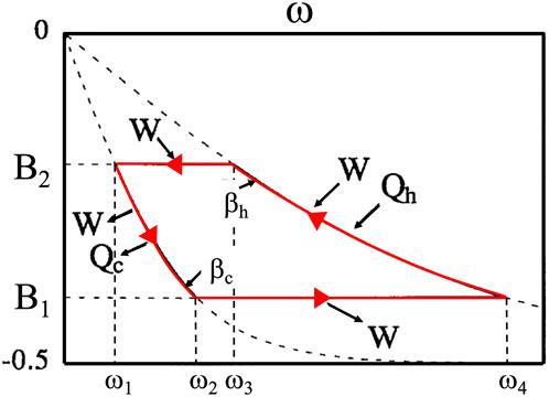
Figure 4. A reversible quantum Carnot cycle depicted in the space of the normalized magnetic field $\omega$ and the magnetization $B$. The horizontal lines represent adiabats wherein the engine is uncoupled from the heat baths at inverse temperatures ${\beta }_{h,c}=1/k_B{T}_{h,c}$, and the magnetic field is changed between two values; the two horizontal strokes represent changing the magnetization $\omega$ while the qubits are connected to a heat bath at constant temperature. The black arrows indicate the direction of heat and work from/to the spin-qubit system. (Adapted with permission from [58]).

The two terms on the right-hand side are to be identified, respectively, with the average work, $⟨\delta W⟩=⟨{\sigma }_z⟩\delta \omega /2$, and average heat, $⟨\delta Q⟩=\omega \delta ⟨{\sigma }_z⟩/2$, exchanged in the analog of the derivation of the First Law (see Eq. 50 below).

Now, consider the extreme situation in which the total magnetic energy of the spin chain increases continuously from the lowest state with all spins “down” to the highest state with all spins “up.” Both the initial and final states have only one microstate available, $\mathrm{\Omega }$ = 1, $p_1$ = 1; therefore, their von Neumann entropy is 0. While the magnetic field spans between these two extremes, the entropy first increases from 0, goes to its maximum when the spins are, on average, half-up and half-down, and then decreases again, going back to 0. Correspondingly, the temperature goes from 0 to plus-infinity at the entropy maximum, then jumps to negative-infinity (because entropy and energy have opposite-sign first derivatives) and goes back to 0, always from negative values.

As Ramsey pointed out (Ramsey, 1956), the number of physical systems actually capable of assuming a negative temperature is limited to systems with a finite number of energy levels and sufficient thermal insulation from positive-temperature reservoirs. In the real world, atomic or nuclear spin systems have other degrees of freedom; if the coupling between the spins and other degrees of freedom is much weaker than the strong coupling between spins, we can talk about a “spin temperature” separately from the temperature of the atoms or lattice as a whole. It is interesting to note that if one can realize a system simultaneously coupled to a positive and a negative thermal bath, Carnot’s efficiency $(1-T_1/T_2)$ could indeed assume values larger than 1 (Geusic et al., 1967).

By using quantum mechanical states as the heat exchanger “fluid,” even a single atom can turn into a Carnot engine, as shown by Singer’s group in Mainz (Rossnagel et al., 2016). Sandwiched between an electric field representing the hot reservoir and a laser cooling beam representing the cold reservoir, a single ⁴⁰${\mathrm{C}\mathrm{a}}^{+}$ ion is caught in a funnel-shaped, magnetic quadrupole linear trap, with frequency ${\omega }_r$. The “temperature” of the ion quantum state is determined by the radial spreading of the wavefunction, approximately Gaussian, with a width $\sigma (T)={(k_{B}T/m{\omega }_r^2)}^{1/2}$. The cooling laser is always on, while the electric field is switched on and off, thereby making the ion temperature oscillate between “cold” and “hot” by sweeping the trap frequency between the extremes $\pm {\omega }_M$A thermodynamic cycle is performed, and work is extracted by the axial force generated by the movement of the trapped ion. Compared to the equivalent Carnot cycle, the efficiency is extremely small, of the order of 0.003; however, the result of a single ion performing as a reversible and essentially frictionless quantum engine is nothing short of amazing.

The same group had previously demonstrated (but not experimentally realized, at least yet) an example of an Otto cycle for a time-dependent oscillator coupled to a “squeezed” thermal reservoir, which could have a theoretical efficiency above Carnot’s limit and approach unity (Rossnagel et al., 2014). There, the squeezing (a common concept in quantum optics (Breitenbach et al., 1997)) refers to the particular construction of the quantum states of the thermal bath, in which the thermal noise is distributed differently among the degrees of freedom. For example, in a harmonic oscillator, the noise can be concentrated in the phase but not in the amplitude (Breitenbach et al., 1997; Esteve et al., 2008).

6.3 Thermal vs. quantum fluctuations

Thermodynamics is an effective macroscopic picture of thermal processes that is not concerned with microscopic details but only deals with average quantities such as temperature, work, and dissipated heat. This classical approach is valid for a macroscopic number of particles in the so-called thermodynamic limit ($N\to \infty ,V\to \infty$, with $N/V=const$), but starts losing accuracy as the system size decreases to a small number of degrees of freedom. In this regime, thermal fluctuations of the average quantities can become as relevant as the averages themselves, or more, because they alone may induce deviations from the average behavior (Alemany and Ritort, 2010). Compared with macroscopic thermodynamics, fluctuations play a much more important role in small systems. However, the presence of fluctuations does not mean that we cannot characterize quantum systems thermodynamically; on the contrary, fluctuations typically contain important additional thermodynamic and energetic information that is usually lost as noise in the infinite-system limit.

Stochastic thermodynamics picks up where the macroscopic description starts to fail and gives insight into the fluctuations of thermodynamic quantities. It also moves beyond the equilibrium situations associated with thermodynamics and can describe the behavior of systems that are out of equilibrium. Considerations stemming from fluctuation theorems (Evans et al., 1993; Jarzynski, 1997; Crooks, 1999) are vital when considering nanoscale devices, or biological protein machines, for which experiments confirmed the theoretical predictions of local violation of the Second Law (Wang et al., 2004). Such “theorems” (in fact, they should be better called “relations” because they do not stem from a rigorous derivation from a set of axioms) state at different levels that for dynamical systems far from equilibrium, there exists a physically meaningful, real-valued variable ${\mathrm{\Omega }}_t$, extensive both in space and time, whose positive values are exponentially more probable than the negative ones, or

$\frac{P\left(+{\mathrm{\Omega }}_t\right)}{P\left(-{\mathrm{\Omega }}_t\right)}=e^{{\mathrm{\Omega }}_t}.(48)$

In practice, this variable is easily identified with entropy production, which is extensive and increasing with time. What such fluctuation relations state, therefore, is that the second law probabilistically holds for a macroscopic system observed over macroscopic times. It can be “violated” (that is, entropy flows in the reverse direction) if the system is sufficiently small and/or the observation time is sufficiently short. In particular, according to Crook’s fluctuation relation (Crooks, 1999), for a transformation between two microscopic states $A$ and $B$ separated by a free energy $\mathrm{\Delta }F$, the thermodynamic work $W$ is a fluctuating quantity and is therefore given by a probability distribution of values. For ideally reversible transformations, the work distributions in the time-forward or backward direction cross at the value $W=\mathrm{\Delta }F$, as clearly demonstrated by optical tweezers experiments on the cyclic folding and unfolding of RNA fragments (Collin et al., 2005).

At an even smaller scale, however, fluctuations are no longer merely thermal but quantum mechanical in origin. In the regime in which quantum phenomena are manifested, that is, very low temperatures and sizes smaller than the De Broglie wavelength, Heisenberg’s uncertainty relations become the relevant source of noise in the form of localized, temporary random changes of the system energy, for a (very) short time. Then, many questions arise when applying such concepts to qubits. For example,

$•$ What becomes of thermodynamic equilibrium for time-reversible, unitary transformations?

$•$ What is the meaning of thermalization in the presence of quantum integrals of motion?

$•$ How to define and/or measure thermodynamic quantities for quantum systems?

$•$ How entanglement is connected with information entropy?

$•$ and more$\dots$

The fluctuations we are after for a quantum system in contact with a heat bath are not strictly thermal ones. Rather, they are represented by combinations of (1) the possible changes in the distributions of the energy levels (that is, a change of the Hamiltonian) and/or (2) changes of their occupation numbers (that is, entropy). In both cases, the result is a degradation of the quantum state, that is, a loss of coherence. The pure state turns into a mixed state.

In the approximation of weak coupling between the quantum system and the thermal bath, the equilibrium density tends to a Gibbs state $(\beta =1/k_{b}T)$:

${\rho }^{eq}=\frac{\exp \left(-\beta \mathcal{H}\right)}{\mathcal{Z}}(49)$

with, as usual, $\mathcal{Z}=\mathrm{Tr}\{\exp (-\beta \mathcal{H})\}$ being the system’s partition function. The average internal energy is $E(\rho )=\mathrm{Tr}\{\mathcal{H}\rho \}$, the entropy is $S=-\mathrm{Tr}\{\rho \ln \rho \}$, and the free energy is obtained as $F=E(\rho )-TS(\rho )=-\ln \mathcal{Z}/\beta$. Hence, a “weak” quantum equivalent of the First Law can be written:

$dE=\delta Q+\delta W=\mathrm{Tr}\left\{\left(d{\rho }^{eq}\right)\mathcal{H}\right\}+\mathrm{Tr}\left\{{\rho }^{eq}\left(d\mathcal{H}\right)\right\}.(50)$

The first term on the right-hand side, containing the differential of the equilibrium density, is relative to a variation of occupation numbers of the quantum eigenstates and is therefore assimilated to a form of thermodynamic entropy analogous to the $\delta Q$ of classical thermodynamics. The second term, in turn, containing the differential of the system Hamiltonian, corresponds to a change in the structure of the energy levels, as it could derive from a change in the system mechanics, and can be assimilated to a work $\delta W$ done on, or by, the quantum system.

6.4 Work and heat are not quantum- mechanical observables

Both quantities are dependent on the process path $\lambda$ (and thus are non-exact differentials, like in classical thermodynamics), which means they do not correspond to quantum mechanical observables; that is, there is no Hermitian operator $\widehat{q}$ or $\widehat{w}$ such that $Q=\mathrm{Tr}\{\rho \widehat{q}\}$ and $W=\mathrm{Tr}\{\rho \widehat{w}\}$. The intuitive, simplistic reasoning behind such a statement is that the final-state Hamiltonian at $t$ = $\tau$ does not necessarily commute with the initial Hamiltonian at $t$ = 0; that is,

$\left[\mathcal{H}\left({\lambda }^t\right),\mathcal{H}\left({\lambda }^{\tau }\right)\right]\ne 0(51)$

for some (or all) times $0<t<\tau$.

A different definition of quantum work (w/r to Eq. 50) can be given as the difference between eigenvalues of the “instantaneous” Hamiltonian at the beginning and end of the path $\lambda$:

$W=\left({ϵ}_m^{{\lambda }_{\tau }}-{ϵ}_n^{{\lambda }_0}\right).(52)$

Here, quantum work is a random variable distributed as $p(W;\lambda )$ and is given by a time-ordered correlation function as a path-dependent quantity. On this basis, the quantum equivalent of the fluctuation theorems can also be recovered (Talkner et al., 2007; Hänggi and Talkner, 2011):

$\frac{p\left(W;\lambda \right)}{p\left(-W;\lambda \right)}=e^{\beta \left(W-\mathrm{\Delta }F\right)}\left(\text{Crooks}\right).(53)$

${⟨e^{\beta W}⟩}_{\lambda }=e^{-\beta \mathrm{\Delta }F}\left(\text{Jarzinsky}\right).(54)$

However, for a quantum system entangled with its environment, the interaction energies are not weak; in fact, they will quickly degrade the pure state into a mixed one in a time of the order of the coherence time. Identification of “heat” and “work” with the variation of the system’s characteristics $(d\rho ,d\mathcal{H})$ is no longer enough. During isothermal quasi-static processes, part of the free energy exchanged with the environment represents an “energetic price” to pay in order to preserve the coherence and quantum correlations in the system. Denoting a non-Gibbsian, coherent and correlated state as ${\rho }^{cc}$, the extended entropy $S_e$ can be written as

$\begin{array}{cc}\hfill S_e& =-\mathrm{Tr}\left\{{\rho }^{cc}\ln {\rho }^{cc}\right\}=\hfill \\ \hfill & =-\mathrm{Tr}\left\{{\rho }^{cc}\ln {\rho }^{cc}\right\}+\left[\mathrm{Tr}\left\{{\rho }^{cc}\ln {\rho }^{eq}\right\}-\mathrm{Tr}\left\{{\rho }^{cc}\ln {\rho }^{eq}\right\}\right]=\hfill \\ \hfill & =\beta \left[E-\left(F+TS\left({\rho }^{cc}\Vert {\rho }^{eq}\right)\right.\right]=\beta \left[E-\mathcal{F}\right]\hfill \end{array}(55)$

(note that the last term in […] in the second line is zero). $S({\rho }^{cc}\Vert {\rho }^{eq})=\mathrm{Tr}\{{\rho }^{cc}(\ln {\rho }^{cc}-\ln {\rho }^{eq})\}$ is the quantum relative entropy (Vedral, 2002), and $\mathcal{F}=F+TS({\rho }^{cc}\Vert {\rho }^{eq})$ is the so-called information free energy (Parrondo et al., 2015). In analogy with the perfect-Gibbs case, consider the non-Gibbsian infinitesimal of $d{S}_e$:

$\begin{array}{cc}\hfill d{S}_e& =\beta \left(dE-d\mathcal{F}\right)=\beta \left(\mathrm{Tr}\left\{\left(d{\rho }^{cc}\right)\mathcal{H}\right\}+\mathrm{Tr}\left\{{\rho }^{cc}\left(d\mathcal{H}\right)\right\}-d\mathcal{F}\right)\hfill \\ \hfill \\ \hfill & \equiv \beta \left(\delta Q_{\mathit{tot}}-\delta Q_{cc}\right)\hfill \end{array}(56)$

where $\delta Q_{\mathit{tot}}=Tr\{(d{\rho }^{cc})\mathcal{H}\}$ is assimilated to the total heat exchanged, and $\delta Q_{cc}=d\mathcal{F}-\mathrm{Tr}\{{\rho }^{cc}(d\mathcal{H})\}$ is the “energetic price” to maintain coherence and correlation.

Then, the “entangled system” quantum equivalent of the first law can now be written as:

$de=d{S}_e/\beta +\delta \mathcal{F}=Tr\left\{\left(d{\rho }^{cc}\right)\mathcal{H}\right\}+\mathrm{Tr}\left\{{\rho }^{cc}\left(d\mathcal{H}\right)\right\}(57)$

This is only formally similar to the previous statement, Eq. 50, and has a peculiarly different meaning of the symbols for $E,S_e,\mathcal{F}$.

6.5 Quantum version of Landauer’s limit

Consider a quantum system $S$ whose information content is progressively erased upon interacting with a quantum environment $E$. Both $S$ and $E$ are living in their respective Hilbert spaces ${\mathcal{W}}_S,{\mathcal{W}}_E$. Assume that the initial state of the composite system is factorized

${\rho }_{SE}\left(0\right)={\rho }_S\left(0\right)\otimes {\rho }_E\left(0\right).(58)$

such that no initial correlations are present. The environment is initially prepared in a thermal Gibbs state ${\rho }_E(0)=\exp (-\beta {\mathcal{H}}_E)/{\mathcal{Z}}_E$. $S$ and $E$ interact via the unitary transformation $U(t)=\exp (-i\mathcal{H}t/\hslash )$, with $\mathcal{H}={\mathcal{H}}_S+{\mathcal{H}}_E+{\mathcal{H}}_{SE}$ the total Hamiltonian comprising the system, the environment, and their interaction.

Landauer’s principle is related to the change in the entropy of the total system plus the environment; therefore, we can reinterpret the heat exchanged between $S$ and $E$ as the difference between their respective initial and final entropy:

$\left[S\left({\rho }_S^t\right)-S\left({\rho }_S^0\right)\right]+\left[S\left({\rho }_E^t\right)-S\left({\rho }_E^0\right)\right]=\mathrm{\Delta }{S}_S-\mathrm{\Delta }{S}_E=\mathcal{I}\left({\rho }_{SE}^t\right)\ge 0(59)$

This is, by definition, also equal to the quantum mutual information exchanged between $S$ and $E$:

$\mathcal{I}\left({\rho }_{SE}^t\right)=S\left({\rho }_E^t\right)+S\left({\rho }_E^t\right)-S\left({\rho }_{SE}^t\right)(60)$

(Note that for a completely factorized initial state, $\mathcal{I}({\rho }_{SE}^t)=0$.) With some algebra (see full derivation in Reeb and Wolf (2014)), it is shown that the average heat dumped from $S$ into the environment, $⟨Q_E⟩=\mathrm{Tr}\{({\rho }_E^t-{\rho }_E^0){\mathcal{H}}_E\}$, is equal to

$\beta ⟨Q_E⟩=\mathrm{\Delta }{S}_S+\mathcal{I}\left({\rho }_{SE}^t\right)+S\left({\rho }_E^t\Vert {\rho }_E^0\right)(61)$

Because both $\mathcal{I}({\rho }_{SE}^t)$ and $S({\rho }_E^t\Vert {\rho }_E^0)\ge 0$, it is also

$\beta ⟨Q_E⟩\ge \mathrm{\Delta }{S}_S(62)$

This important relationship, therefore, establishes that the only heat dissipation in quantum computing occurs during state initialization and reset (erasure) operations, which are both linear in the number of qubits: the entropy changes in the quantum system turn into heating of the environment, by an amount simply proportional to the number of qubits and not to the dimension of their Hilbert space. That is quite good news because for $N$ qubits, the Hilbert space has dimension $2^N$ or, in other words, $2^N$-distinct possible eigenstates, a number that grows very quickly. A classical computer simulating this quantum computer, instead, must use an energy at least equal to $2^N{k}_{B}T\ln$2 simply to initialize or erase the configuration. Hence, this represents an additional bound to quantum advantage for a given classical calculation.

Eq. 62 has been verified experimentally in several cases. In Figure 5 the results of two such experiments are reported (Yan et al., 2018; Cimini et al., 2020).

Figure 5

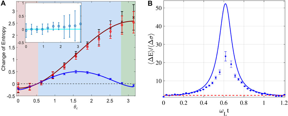
Figure 5. (A) Experimental verification of Eq. 62 on a ⁴⁰Ca ion-trap qubit. Black data $=\beta ⟨Q_E⟩$; red data $=\mathrm{\Delta }{S}_S+\mathcal{I}({\rho }_{SE}^t)+S({\rho }_E^t\Vert {\rho }_E^0)$ (reprinted with permission from Yan et al. (2018)). (B) The $\beta ⟨Q_E⟩\ge \mathrm{\Delta }{S}_S$ limit demonstrated experimentally on a toy-model optical qubit gate. [Reprinted with permission from Cimini et al. (2020)].

6.6 Thermalization: randomization of pure states into mixed states

The typical initial condition of a quantum computer is a pure state, for example, with all the qubits prepared in the same state $|{\psi }_i\rangle =\left(1/0\right)$ for $i\in N$, by a previous RESET operation. As we saw in the subsection above, this operation costs both energy and heat, but it is fortunately linear with $N$. Quantum decoherence explains how a system interacting with an environment transitions from being a pure state (that exhibits coherent superpositions) to a mixed state, which is an incoherent combination of classical alternatives. The transition is ideally reversible, as the combined state of the system and environment may still be a pure state. However, for all practical purposes, it should be seen as irreversible, as the environment is, in general, a very large and complex quantum system, and it is not practically feasible to reverse their interaction.

A general description of the transformations between states when the quantum system interacts with an external environment can be given by a kind of master equation first introduced by Lindblad (1976). Such dynamics preserve the trace and positivity of the density matrix while allowing the density matrix to vary otherwise (Breuer and Petruccione, 2002). Master equations have the general form (Manzano, 2020):

$\frac{d\rho }{dt}=-\frac{i}{\hslash }\left[\mathcal{H},\rho \right]+{\displaystyle \sum _k}\left[L_k\rho L_k^{†}-\frac{1}{2}\left(L_k^{†}{L}_k\rho +\rho L_k{L}_k^{†}\right)\right].(63)$

(to be compared with Eq. 33 above). The $L_k$ are Lindblad operators that describe the effect of the interaction between the system and the environment on the system’s state. A good example is the interaction of the 1/2-spin qubit with an electromagnetic field, for which there is only one operator $L={\sigma }^{+}$, $L^{†}={\sigma }^{-}$, which applied on the qubit gives ${\sigma }^{-}|0\rangle =|1\rangle$ and ${\sigma }^{+}|1\rangle =|0\rangle$. The external photon field is described by a spontaneous emission rate ${\gamma }_0$, with number density $N$ given by the Bose–Einstein distribution:

$N=\frac{1}{e^{\beta \omega }-1}(64)$

and $\gamma ={\gamma }_0(2N+1)$ is the total emission rate, including thermally induced absorption and emission at the temperature $\beta =1/k_{B}T$(Cherian et al., 2019; Jäger et al., 2022). The master equation describing the evolution is

$\frac{d\rho }{dt}=-\frac{i}{\hslash }\left[\mathcal{H},\rho \right]+{\gamma }_0\left(N+1\right)\mathcal{D}\left({\sigma }^{-}\right)+{\gamma }_{0}N\mathcal{D}\left({\sigma }^{+}\right)(65)$

where the more compact “dissipator” notation $\mathcal{D}(L)=L\rho L^{†}-\frac{1}{2}\{L^{†}L,\rho \}$ has been introduced. Figures 6A,B compare the evolution of the density matrix $\rho (t)$ in the two cases: (a) under the action of Eq. 33, with the unitary Hamiltonian ${\mathcal{H}}_0=\hslash \omega {\sigma }_z/2$ and (b) the dissipative Eq. 65. All the unitary Hamiltonian does is a precession of the state vector around $z$; on the other hand, upon coupling to the dissipator operator, the precession is accompanied by a damping towards the $z$-axis. (Side note: The Hamiltonian for a spin population pumped by a coherent laser source, $\mathcal{H}={\mathcal{H}}_0+\frac{\lambda }{2}({\sigma }^{+}+{\sigma }^{-})$, is still unitary and Hermitian (the rates of upward and downward transitions are equal); the result is simply a precession about an axis inclined w/r to $z$. See the dashed line in Figure 6A).

Figure 6

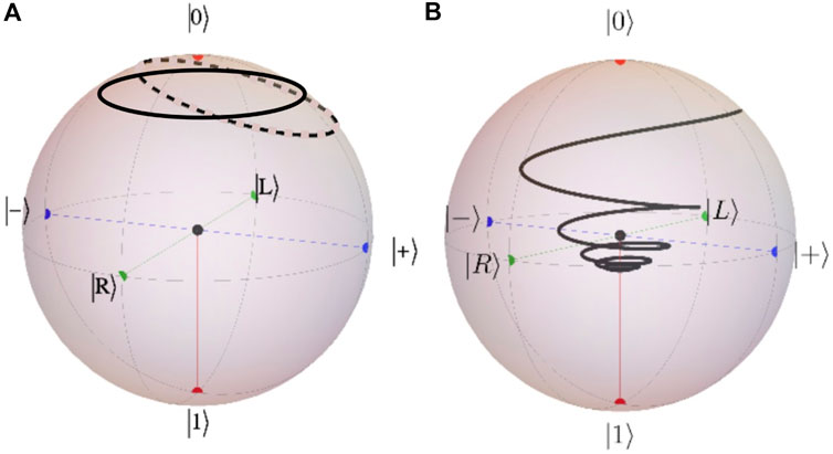
Figure 6. (A) Unitary dynamics from Eq.33 and (B) dissipative dynamics from Eq. 65 in the Bloch sphere. (Adapted from G.T. Landi, with permission).

It is worth noting that the time-independent generator in Lindblad form describes the memoryless dynamics of the open system, typically leading to an irreversible loss of characteristic quantum features. However, in many applications, open systems exhibit pronounced memory effects in the more general framework of non-Markovian quantum dynamics (Breuer et al., 2016). Typically, this is because the relevant environmental correlation times are not small compared to the system’s relaxation or decoherence time, thus rendering the standard Markov approximation not applicable. The violation of this separation of time scales can occur, for example, in the cases of strong system–environment couplings, structured or finite reservoirs, low temperatures, or large initial system–environment correlations (see, e.g., Verstraete et al. (2009); Hanson et al. (2008); Zhang et al. (2017); Shen et al. (2013)).

Decoherence describes the classical limit of quantum mechanics but is different from wavefunction collapse. In the mixed state, all classical alternatives are still present, whereas the wavefunction collapse (i.e., a measurement) selects only one of them (Hill and Wootters, 1997; Wootters, 1998). Consider two qubits $A$ and $B$ (e.g., spin-1/2 particles or polarized photons) characterized by an excitation energy $E$ at a temperature $k_{B}T=1/\beta$, so that the thermal probability of the excited state is $p={[1+\exp (-\beta E)]}^{-1}$. Both a pure and a mixed state can be entangled over the ensemble of their qubits; however, the difference between the two cases is important. As already said above, a pure state is called entangled when it is unfactorizable. One of the simplest definitions of entanglement of a pure state can be given as the (von Neumann) entropy of either member of the pair. A mixed state, on the other hand, is called entangled if it cannot be represented as a mixture of factorizable pure states. The entanglement of a mixed state $\rho$ is the minimum average entanglement of an ensemble of pure states that represents $\rho$.

The entanglement of formation ${ϵ}_f(\rho )$ of the mixed state $\rho$ is the amount of resources needed to create a given entangled state (Bennett et al., 1996). ${ϵ}_f(\rho )$ is defined as the average entanglement between pure states of the decomposition, minimized over all the decompositions ${\psi }_i$ of $\rho$ (Verstraete et al., 2001):

${ϵ}_f\left(\rho \right)=\min {\displaystyle \sum _i}{p}_{i}S\left({\psi }_i\right)=S_e\left[\frac{1}{2}\left(1+\sqrt{1-C}\right)\right](66)$

also related to a different measure of entanglement, the concurrence $C(\rho )$, via the Shannon entropy $S_e$.

Maximally entangled states of a pair of qubits (Bell states) can be constructed in a quantum computation, as we saw in Section 3 above, by applying a Hadamard gate (rotation) followed by a CNOT; let us call these two unitary operators $U_1$ and $U_2$. Starting from an initial density ${\rho }_i$, the final maximally entangled state is ${\rho }_f=U_2{U}_1{\rho }_i{U}_1^{†}{U}_2^{†}$ (Verstraete et al., 2001). What is interesting to note here is that after some algebra, the concurrence of the final state can be obtained explicitly as

$C=\max \left(\mathrm{0,2}{p}^2-p-2\left(p-1\right)\sqrt{p\left(1-p\right)}\right)(67)$

This suggests the existence of an “entanglement threshold:” for $p\lesssim 0.698$, or equivalently for $k_{B}T/E\gtrsim 1.19$, no entangled state of two qubits can be produced. For the typical transmon excitation energy of the order of $E$ = 4 GHz, the maximum entanglement temperature is $T\simeq$240 mK. Note that this limit is well above the working temperature of SC loops, approximately 10–20 mK, while trapped-ion qubits are operated at even lower liquid-He temperatures.

6.7 Many qubits, multipartite systems

We can associate to every unitary operation $U$ a work cost $W=\mathrm{Tr}\mathcal{H}({\rho }^f-{\rho }^i)$, which corresponds to the external energy input required to perform that operation. Think of two qubits $A$ and $B$ in the same thermal state at a temperature $T=1/\beta$; their initial thermal state is joint, so we can write ${\rho }_{AB}(\beta )={\rho }_A(\beta )\otimes {\rho }_B(\beta )$, but their Hamiltonian is non-interacting, ${\mathcal{H}}_{AB}={\mathcal{H}}_A+{\mathcal{H}}_B$. To entangle (correlate) them, we must bring the joint system out of equilibrium. Necessarily, $W>0$ for every possible $U$ because the initial state is in thermal equilibrium. Then, a relevant question is: what is the minimal work cost for correlating thermal states? Or, equivalently, what is the maximal number of attainable correlations when the energy at our disposal is necessarily limited?

The result of a limiting temperature for the entanglement of a pair of qubits, obtained from Eq. 67, can be generalized to the case of multiple qubits (Huber et al., 2015). Consider $N$ qubits and the rotation (Hadamard) from a pure to a maximally entangled state in the subspace $|{0\rangle }^{\otimes N}$, $|{1\rangle }^{\otimes N}$. Next, consider the possible bipartitions of the system $(j|N-j)$, for which we consider a subpart of the system of $j<N$ qubits entangled with its complement $N-j$. It has been shown that the concurrence is, in fact, independent of the particular choice of the bipartition and depends only on the system size:

$C=p^N-{\left(1-p\right)}^N-2p^{N/2}{\left(1-p\right)}^{N/2}.(68)$

Again, we ask what is the smallest thermal factor $p_b={[1+\exp (-E/k_B{T}_b)]}^{-1}$, or the maximum temperature $k_B{T}_b=1/{\beta }_b$, which allows simultaneously obtaining entanglement across all the possible bipartitions of the system? By imposing $C$ to be positive, that is

$\frac{1}{{\beta }_{b}E}\ge \frac{N}{2\ln \left(1+\sqrt{2}\right)},(69)$

the corresponding work of correlation for the maximally entangled set is

$W=NE\frac{\left(1-e^{-N{\beta }_{b}E}\right)}{2{\left(1+e^{-{\beta }_{b}E}\right)}^N}=NE\frac{1+\sqrt{2}}{{\left[{\left(1+\sqrt{2}\right)}^{2/N}+1\right]}^N}(70)$

which is exponentially small in the number of qubits $N$. This interesting result proves that by increasing the number of qubits, it becomes possible to generate partial entanglement even at (arbitrarily) high temperatures. This is because typical gate protocols act on qubit subspaces, whose population becomes negligible in the limit of large $N$. Therefore, even a small amount of entanglement obtained on a subset of the available states might be enough to obtain a substantial quantum advantage.

How many correlations can be induced in a system of many qubits? In addition, how can we make sure that a set of qubits is actually entangled? This is the more general problem of entanglement detection (Guhne and Toth, 2009). A measure of the total number of correlations gives the deviation of the global state of the quantum computer from a corresponding uncorrelated state, a quantity that is important to estimate in the preparation of the initial correlated state. The total system composed of $k$ subsystems will be said to have zero correlation if its state is such that $\rho =\otimes {\rho }_i$, $i\in k$, that is, the direct product of its partials. Therefore, a common measure of the correlation can be given by the relative entropy of the state (Bennett et al., 2011; Goold et al., 2016; Girolami et al., 2017):

$S_{\mathit{rel}}\left(\rho \right)={\displaystyle \sum _i}{S}_i\left({\rho }_i\right)-S\left(\rho \right).(71)$

Despite its apparent simplicity, such a measure is highly non-linear and difficult to access in a real experimental device with more than only a few qubits, so alternative approaches have been proposed, based, for example, on the Rényi entropy (Brydges et al., 2019), the measurement of “witness” observables (Guhne and Toth, 2009; Friis et al., 2019), or more general quantifiers including the notion of “fidelity” (Liang et al., 2019; Liu et al., 2022).

6.8 The supremacy clause of quantum thermodynamics

As was briefly discussed in Section 4, the fundamental noise limit for classical computers is of thermal origin, with a contribution $\mathcal{O}(k_{B}T)$. To prevent random bit flipping, the excitation energy $E$ needs to be sufficiently larger than the thermal energy $k_{B}T$. Under reasonable assumptions, the error probability in assigning a state to a classical bit is (Kish, 2002)

${ϵ}_Q\gtrsim \exp \left(-E/k_{B}T\right).(72)$

For a quantum computer with gates driven by auxiliary oscillators at frequency $\omega$ (with $\omega >2\pi /\tau$, and $\tau$ the coherence time), the corresponding lower error limit is (Gea-Banacloche, 2002b)

${ϵ}_Q\gtrsim \frac{\hslash \omega }{E}>\frac{h}{E\tau }.(73)$

It can be noted that this is a sort of generalized time–energy uncertainty relation, describing the minimum energy needed to change a state in a time less than $\tau$ with failure probability smaller than ${ϵ}_Q$. The meaning of this comparison is that in the quantum case, the error decreases only in inverse proportion to the energy used, while in the classical case, it decreases exponentially. The quantum regime corresponds to $\hslash \omega >k_{B}T$, that is, when the quantum noise in the driving oscillator exceeds the thermal noise at the work temperature.

Because of quantum reversibility, the excitation energy $E$ need not be dissipated; it only needs to be put into and removed from the driving system to switch on and off the desired gate evolution. In theory, if nothing is ever erased, “conservative” computation is possible. However, there are two caveats. First, any proposed quantum computer architecture to date has no mechanisms to actually “recycle” that energy. Current SC gates are based on microwave power pulses, which obviously consume energy irreversibly. However, any practical computer, even if it could use fully reversible gates, is still going to generate heat, at least because of error correction to keep the computation on track. Error correction inherently requires irreversible operations, such as supplying continuous ground-state configurations (e.g., “zero” ancilla qubits). Reversible circuits must be adiabatic; there cannot be heat exchanges between the circuit and its environment. They must be in equilibrium at all times, which means conserving the squared modulus of the wavefunction, and “all times” actually means during the coherence time.

Two universal reversible logic gates, both operating on three bits or qubits, have been suggested for the implementation of logically reversible operations. The Toffoli gate (Toffoli, 1982) inverts the state of a target bit conditioned on the state of two control bits; the Fredkin gate (Fredkin and Toffoli, 1982) swaps the last two bits conditioned on the state of the control bit. In these two gates, any set of inputs is processed and results in a unique pattern of outputs; these gates are, therefore, logically reversible. Examples of logically reversible circuits have actually been designed and fabricated (Shao et al., 2007; Orbach et al., 2012; Patel et al., 2016; Li et al., 2022); however, they always practically display some degrees of energy dissipation by different means (e.g., requiring ancilla qubits (Ikonen et al., 2017), finite-rate operation and read-out (Orbach et al., 2012), and so on).

Second, and most importantly, this much excitation energy to prepare the initial state, even if in principle recyclable, must be fully available at least to start the calculation. If we assume as a practical upper bound ${ϵ}_Q\simeq 10^{-5}$ and a GHz quantum computer, the minimum (reversible) $E$ per elementary logical operation is then $\sim$0.007 eV, compared to the thermal energy $\sim 10^{-6}$ eV at 30 mK. As a worst-case example (Gea-Banacloche, 2002a), let us suppose that 5,000 logical qubits are needed to factor a 1000-bit number, a seven-qubit code concatenated only once (depth = 2) is used for error correction, only local gates are available, and approximately 10 ancilla qubits per logical qubit are used. Figure 7 shows estimates of the minimum power as a function of coherence time for a driving microwave field at frequency $\omega ={({ϵ}_Q^{3/2}\tau )}^{-1}$. The full and dashed lines correspond to periodic and static excitation fields.

Figure 7

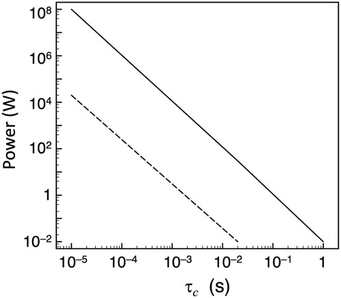
Figure 7. Estimate of the minimum power required to factor a 1000-bit number, as described in the text. Solid line: oscillatory control fields, $\omega ={({ϵ}_Q^{3/2}\tau )}^{-1}$. Dashed line: static control fields only. [Reprinted with permission from Gea-Banacloche (2002a)].

Despite the purely heuristic nature of Eq. 73 (for example, the error limit could be improved by smarter correction algorithms or by improved hardware solutions), the results clearly indicate that, for very large-scale quantum computations, one must use quantum systems with very long decoherence times. Values of $\tau$ in the 100-$\mu$s range would require megawatt start-up power. It is simply not feasible to get around the problem of short decoherence times merely by driving the system at faster frequencies. This also suggests that there could probably never be the equivalent of a “Moore’s law” for quantum computers.

The energy budget that would be required for large-scale quantum applications has only sparely been considered. Efficiency, quantum advantage, or quantum supremacy are most often estimated in terms of the amount of resources needed for a quantum vs. classical computation (number of qubits, connections, scaling of the operations). However, the final bill from the electric company will eventually count the watt-hours consumed, and the notion of “green quantum advantage” provides a more useful comparison by looking at the number of elementary operations performed per watt consumed (Bedingham and Maroney, 2016; Jaschke and Montangero, 2023). A key quantity to consider is the amount of energy needed to implement a quantum gate in a set amount of time (Cimini et al., 2020; Deffner, 2021; Stevens et al., 2022; Fellous-Asiani et al., 2023). While the main concern of fundamental quantum computing is focused on the issues of noise reduction and protecting quantum resources from decoherence, the management of resources at the full-stack, macroscopic level must take into account all the enabling technologies that surround the quantum machine and make it possible to interact with and extract information from it. Quantum thermodynamics is but one brick of the construction that will lead to the future of quantum computers; however, as it can be demonstrated by comparing with the historical trajectory of classical CMOS computers, the issues around energy consumption of quantum computing represent a crucial step that must be faced even well before any practical machine will be operational (Aufféves, 2022; Carlesso and Paternostro, 2023).

6.9 Objectivity of measurement and “Quantum Darwinism”

In the standard circuit (or QED) model, the array of qubits is initialized, for example, in the logical $|0\rangle$ state; then, a sequence of quantum gates is applied depending on the required algorithm; finally, a read-out operation is carried out by measuring individual qubits in the same $|0/1\rangle$ computational basis. In the alternative, the adiabatic quantum computation does not rely on gate sequences but on the direct implementation of a smoothly varying Hamiltonian on the network of qubits after the initial prepared state, annealing, and read-out are cyclically performed to obtain the global optimum configuration of spins, which gives the ground state of the “solution” Hamiltonian. In either instance, the read-out operations give a human-readable, classical physics result from the quantum computation.

The final state of the computation is something like $|\psi \rangle ={\sum }_n{c}_n|n\rangle$ and, as we know, the complex amplitudes $c_n$ are not directly accessible. The measurement gives one of the $n\in N$ possible outcomes with probability $|c_n{|}^2$, which is a probabilistic rule for projecting the state vector onto one of the vectors of the orthonormal measurement basis. Consider, for example, the general qubit state $|\psi \rangle =c_1|0\rangle +c_2|1\rangle$, and assume that we want to perform a measurement in the orthonormal basis $|u\rangle =a|0\rangle +b|1\rangle$, $|v\rangle =b^{*}|0\rangle -a^{*}|1\rangle$. The probability of a measurement giving $|u\rangle$ as a result is

$P\left(u\right)=|⟨u,\psi ⟩{|}^2=|\left(a^{*}\langle 0|+b^{*}\langle 1|\right)\left(c_1|0\rangle +c_2|1\rangle \right){|}^2=|a^{*}{c}_1+b^{*}{c}_2{|}^2(74)$

and similarly, the probability of getting $|v\rangle$:

$P\left(v\right)=|⟨v,\psi ⟩{|}^2=|\left(b\langle 0|-a\langle 1|\right)\left(c_1|0\rangle +c_2|1\rangle \right){|}^2=|b{c}_1-a{c}_2{|}^2(75)$

Decoherence of the qubits is the loss of their typical quantum properties, entanglement, and non-locality through interactions with the environment. New correlations with the thermal bath degrees of freedom appear, which degrade the information originally encoded in the quantum system.

In classical physics, what you see is simply “how things are.” You can measure a tennis ball traveling at 120 km/h in a given direction, passing through a given point in space at a given instant of time. What more is there to say? But when a quantum particle is in a state of “superposition” before the measurement, the various superposed states interfere with one another in a wavelike manner. We only see one of these outcomes when we make a measurement. However, given the probabilistic nature of the result, why only that one? Could someone else check our result and find the same outcome?

The definite properties that we associate with classical physics, such as position and velocity, may be selected from a “menu” of quantum possibilities in a process loosely analogous to natural selection in evolution. The quantum properties that survive are—in a kind of pseudo-Darwinist sense—the “fittest” (Zurek, 1982, 2003). As it happens in natural selection, the “survivors” are those that make the most copies of themselves. Many independent observers can thus make measurements of the quantum system, each one using a different copy of the result, and agree on the outcome—a hallmark of classical behavior. “Quantum Darwinism” (QD, Zwolak et al. (2009); Milazzo et al. (2019); Chen et al. (2019); Ryan et al. (2021)) changes the role of the environment from being a shady background with undetermined characteristics into a fragmented space filled with redundant information that can be accessed and “measured” by individual observers. Notably, this notion is different from the macroscopic limit because the number of degrees of freedom of the environment is so large that the averaging process dominates the read-out process. Instead, QD deals with the mechanism by which the quantum information becomes encoded (i.e., entangled) to the surrounding quantum states of the environment.

Experimental measurements of the result of a quantum computation are typically recorded by collecting information transmitted through some carriers—photons, electrons, phonons—that constitute the environment (thermal bath). While there will be many such individual information carriers, only a small fraction typically needs to be captured in order for the observer to accurately record the measurement. Given two observers, they will agree on the outcome when they can independently intercept different fractions of these information carriers and both perform the same type of measurement on their respective sets. In the QD scheme, they will necessarily arrive at the same conclusion due to the entanglement shared between the system and all the environmental degrees of freedom. Then, a key question is whether it is possible to get enough information by monitoring only a small part of the environment.

We may look at the amount of (Shannon) entropy that is produced by destroying the correlations between the system $S$ and a fraction $m\in N$ of the total environment $E$, that is, the quantum mutual information $\mathcal{I}$ defined in Eq. 60 above, and ask how the partial information gathered compares to the whole (Blume-Kohout and Zurek, 2005). From the obvious condition that ${\mathcal{I}}_m$ must be non-decreasing, three possible behaviors can be envisaged as shown in Figure 8A: the linear one, ${\mathcal{I}}_m\propto m$, in which each fraction of the environment provides unique and independent information so that each observer would obtain separate information about the system; alternatively, curve 2, describing redundantly stored information, ${\mathcal{I}}_m$ rapidly increases, then plateaus at the value for which all observers essentially obtain the same information (the so-called “objectivity plateau”); or curve 3, describing information about the system that is tightly encoded so that ${\mathcal{I}}_m$ remains close to zero, then suddenly increases to the maximum around some characteristic amount, for example, $m\sim N/2$.

Figure 8

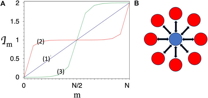
Figure 8. (A) Typical behavior of the information plots ${\mathcal{I}}_m$ as a function of the fractions of environment interrogated by different observers. (B) The spin star environment.

Let us consider a quantum system $S$ of a single qubit initially in a pure state, superposition of two states $|{\psi }_1\rangle ,|{\psi }_2\rangle$ expressed in the conventional basis $|0/1\rangle$ (for the sake of simplicity, I avoid here the customary introduction of the “pointer” states):

$|{\psi }_S\rangle =a|{\psi }_1\rangle +b|{\psi }_2\rangle ,|a{|}^2+|b{|}^2=1(76)$

and embedded in an “environment” of $N$ other qubits, all in a same generic state $|{\psi }_E\rangle$, also expressed in the same basis $|0\rangle ,|1\rangle$ but with random coefficients. The overall initial state is assumed to be without correlation between $S$ and $E$, that is, factorizable as

$|{\psi }_{SE}^0\rangle =\left(a|{\psi }_1\rangle +b|{\psi }_2\rangle \right)\otimes |{\psi }_E\rangle (77)$

QD posits that, after some thermalization time, in which the coupled $S-E$ system evolves, the total state of the system can be turned to

$|{\psi }_{SE}^t\rangle =a|1\rangle |1^{\otimes N}\rangle +b|0\rangle |0^{\otimes N}\rangle (78)$

The notation $M^{\otimes N}=M\otimes M\dots \otimes M$ indicates the direct product of all environment degrees being in either one or the other state of the computational basis.

Several authors have considered the configuration as a “spin star” (e.g., Giorgi et al. (2015); Ryan et al. (2021), see Figure 8B), in which the single qubit is a spin surrounded by a circle of environmental spins. Different subgroups of environment spins can be read out by different observers without perturbing the central spin, which interacts independently and equally with each one of the subsystems.

If we now take the partial trace over the $N$ qubits (spins) of the environment, the density matrix for $S$ is obtained:

${\rho }_S=|a{|}^2|{\psi }_1\rangle \langle {\psi }_1|+|b{|}^2|{\psi }_2\rangle \langle {\psi }_2|(79)$

while each of the environment qubits has the same density matrix:

${\rho }_{E_i}=|a{|}^2|0\rangle \langle 0|+|b{|}^2|1\rangle \langle 1|(80)$

The crucial point is that although the system $S$ has lost its coherence, the population coefficients $(a,b)$ of the qubit $S$ are “imprinted” on each of the $N$ environment qubits, generating a redundancy of information. This is the phenomenon manifested in the “plateau” of constant information seen in Figure 8A, curve (2). Then, different observers measuring only a subset of the final state will agree on the result. This should represent the emergence of classical objectivity.

7 Conclusion

This overview tried to provide a (necessarily limited and incomplete) synthesis of some outstanding issues in the definition of thermodynamic concepts at the level of quantum mechanics, under the peculiar angle of their possible and likely impact on quantum computer technology and quantum computing algorithms. This field has known rapid growth in the past decades, moving from the domain of theoretical speculations to the urgent need to provide real solutions to practical problems that quantum computing hardware is facing. Even though the main technical difficulties today still lie in the probabilistic nature of the quantum computing output and the need for error correction, it is possible that thermal limits will represent the next hurdle for the efficient and useful operation of such machines.

It may be surprising that the historical and philosophical discussions about the second law of thermodynamics should be of interest to, and even represent a foundation for, practical quantum computing. The relationship between information theory, manipulation of information at small scales (which also interests other fields, such as molecular and DNA-based computing; see, for example, Kempes et al. (2017) and Daley and Kari (2002)), and thermodynamics is not purely formal but treats information as a physical entity. The contribution of fluctuation theorems and stochastic thermodynamics provides a more ample framework for analyzing quantum information and exchanges of work and heat in open quantum systems. The definition of quantum entropy (von Neumann’s, despite some ambiguities or other competing definitions) is also key in the attempt to understand the emergence of macroscopic information in the measurement process.

Still, several problems and questions remain at both the fundamental and applied physics levels. For example, the definition of quantum equivalents of work and heat given in Eq. 50 and the path-integral form in Eq. 52 refer to different situations. Meanwhile, the latter fluctuation-based concept is applicable in general to either closed or open systems; the “weak” form refers to the average energy exchanges (ensemble averages) in and out of the system. In most cases, these (and several other) different definitions arrive in practice at the same results; however, our understanding of the question still appears not solid enough and is open to further investigation.

At first, entanglement seems to be unrelated to thermodynamics. However, the challenge of maintaining entangled states is linked to the interaction of qubits with the environment, that is, a thermal bath. Quantum decoherence, or the loss of off-diagonal components in the density matrix, is the process that eventually undermines entanglement by the transfer of entangled states between the computing qubits and the environment’s quantum states. There is a whole thermodynamic domain that I did not touch in this article, quantum batteries (Bhattacharjee and Dutta, 2021; Shi et al., 2022), whose key problem is quantifying the maximum extractable work and which crucially depends on the interplay of coherence and entanglement between the quantum battery and the charger.

Quantum computers can check and verify the theoretical predictions of quantum thermodynamics, and quantum thermodynamics will, in turn, help quantify and master dissipative processes in quantum computing. The interplay of quantum mechanics and thermodynamics is a young research field that is still rich in interesting issues and open questions.

Author contributions

FC: Methodology, writing–original draft, and writing–review and editing.

Funding

The author(s) declare that financial support was received for the research, authorship, and/or publication of this article. Funding from the Science Ouverte-APC grant of the University of Lille is gratefully acknowledged.

Acknowledgments

I gratefully thank my colleagues Valérie Vallet and Stephan De Bievre for their kind invitation to the Quantum Information Working Group at the University of Lille, which provided the excuse to assemble these lectures. Several useful discussions with Stefano Giordano (IEMN) are also gratefully acknowledged.

Conflict of interest

The author declares that the research was conducted in the absence of any commercial or financial relationships that could be construed as a potential conflict of interest.

Publisher’s note

All claims expressed in this article are solely those of the authors and do not necessarily represent those of their affiliated organizations, or those of the publisher, the editors, and the reviewers. Any product that may be evaluated in this article, or claim that may be made by its manufacturer, is not guaranteed or endorsed by the publisher.

Footnotes

¹An extended and updated version of a series of lectures given between January and April 2022 at the Quantum Information Working Group at the University of Lille, France.

²In these experiments, atoms such as ⁸⁷Rb or ¹³³Cs are used, which do not look like bosons. At low temperatures, however, electrons and the nucleus behave as a unique ensemble so that the Rb spin-3/2 nucleus plus the 37 spin-1/2 electrons make up a single system with an integer spin.

³This may be true for pure states and many expectation values, such as energy, but it is not always the case. Consider, for example, the mixed state $\psi =a_1{\varphi }_1+a_2{\varphi }_2$: its $|\psi {|}^2=|a_1{|}^2|{\varphi }_1{|}^2+|a_2{|}^2|{\varphi }_2{|}^2+(a_1^{\ast }{a}_2{\varphi }_1^{\ast }{\varphi }_2+c.c.)$ depends on the phase because $a_1^{\ast }{a}_2=|a_1\Vert a_2|e^{i({\theta }_2-{\theta }_1)}$. The energy of such a mixed state has periodic oscillations at the frequency $\omega =(E_2-E_1)/\hslash$ because of the rotating phase.

⁴Until around 1850, heat and work were considered to be distinct subjects. The experimentally observed asymmetry was the reason why Lord Kelvin initially did not accept the equivalence of work and heat and rather expanded on Clapeyron’s theory of a reversible heat engine (Saslow, 2020).

References

Aaronson, S., and Arkhipov, A. (2011). “The computational complexity of linear optics,” in Stoc ’11: proceedings of the forty-third annual ACM symposium on theory of computing. Editors L. Fortnow, and S. Vadhan (New York, NY: ACM), 333–342.

CrossRef Full Text | Google Scholar

Aghaee, M., Akkala, A., Alam, Z., Ali, R., Ramirez, A. A., Andrzejczuk, M., et al. (2023). InAs-Al hybrid devices passing the topological gap protocol. Phys. Rev. B 107, 245423. doi:10.1103/physrevb.107.245423

CrossRef Full Text | Google Scholar

Agrawal, M., Kayal, N., and Saxena, N. (2004). PRIMES is in P. Ann. Math. 160, 781–793. doi:10.4007/annals.2004.160.781

CrossRef Full Text | Google Scholar

Alemany, A., and Ritort, F. (2010). Fluctuation theorems in small systems: extending thermodynamics to the nanoscale. Europhys. News 41, 27–30. doi:10.1051/epn/2010205

CrossRef Full Text | Google Scholar

Amico, M., Saleem, Z. H., and Kumph, M. (2019). Experimental study of Shor’s factoring algorithm using the IBM Q Experience. Phys. Rev. A 100, 012305. doi:10.1103/physreva.100.012305

CrossRef Full Text | Google Scholar

Anaya-Contreras, J. A., Moya-Cessa, H. M., and Zúniga-Segundo, A. (2019). The Von Neumann entropy for mixed states. Entropy 21, 49. doi:10.3390/e21010049

PubMed Abstract | CrossRef Full Text | Google Scholar

Araki, H., and Lieb, E. H. (1970). Entropy inequalities. Commun. Math. Phys. 18, 160–170. doi:10.1007/bf01646092

CrossRef Full Text | Google Scholar

Arute, F., Arya, K., Babbush, R., Bacon, D., Bardin, J. C., Barends, R., et al. (2019). Quantum supremacy using a programmable superconducting processor. Nature 574, 505–510. doi:10.1038/s41586-019-1666-5

PubMed Abstract | CrossRef Full Text | Google Scholar

Aufféves, A. (2022). Quantum technologies need a quantum energy initiative. PRX Quantum 3, 020101. doi:10.1103/prxquantum.3.020101

CrossRef Full Text | Google Scholar

Bedingham, D. J., and Maroney, O. J. E. (2016). The thermodynamic cost of quantum operations. New J. Phys. 18, 113050. doi:10.1088/1367-2630/18/11/113050

CrossRef Full Text | Google Scholar

Bender, C. M., Brody, D. C., and Meister, B. K. (2000). Quantum mechanical Carnot engine. J. Phys. A Math. Gen. 33, 4427–4436. doi:10.1088/0305-4470/33/24/302

CrossRef Full Text | Google Scholar

Benenti, G., Casati, G., Saito, K., and Whitney, R. S. (2017). Fundamental aspects of steady-state conversion of heat to work at the nanoscale. Phys. Rep. 694, 1–124. doi:10.1016/j.physrep.2017.05.008

CrossRef Full Text | Google Scholar

Bennett, C. H. (1982). The thermodynamics of computation - a review. Int. J. Theor. Phys. 21, 905–940. doi:10.1007/bf02084158

CrossRef Full Text | Google Scholar

Bennett, C. H., DiVincenzo, D. P., Smolin, J. A., and Wootters, W. K. (1996). Mixed-state entanglement and quantum error correction. Phys. Rev. A 54, 3824–3851. doi:10.1103/physreva.54.3824

PubMed Abstract | CrossRef Full Text | Google Scholar

Bennett, C. H., Grudka, A., Horodecki, M., Horodecki, P., and Horodecki, R. (2011). Postulates for measures of genuine multipartite correlations. Phys. Rev. A 83, 012312. doi:10.1103/physreva.83.012312

CrossRef Full Text | Google Scholar

Bernstein, E., and Vazirani, U. V. (1997). Quantum complexity theory. SIAM J. Comput. 26, 1411–1473. doi:10.1137/s0097539796300921

CrossRef Full Text | Google Scholar

Bèrut, A., Arakelyan, A., Petrosyan, A., Ciliberto, S., Dillenschneider, R., and Lutz, E. (2011). Experimental verification of Landauer’s principle linking information and thermodynamics. Nature 483, 187–189. doi:10.1038/nature10872

CrossRef Full Text | Google Scholar

Bespalov, V. A., Dyuzhev, N. A., and Kireev, V. Y. (2022). Possibilities and limitations of CMOS technology for the production of various microelectronic systems and devices. Nanobiotech. Rep. 17, 24–38. doi:10.1134/s2635167622010037

CrossRef Full Text | Google Scholar

Bhattacharjee, S., and Dutta, A. (2021). Quantum thermal machines and batteries. Eur. Phys. J. B 94, 239. doi:10.1140/epjb/s10051-021-00235-3

CrossRef Full Text | Google Scholar

Blais, A., Grimsmo, A. L., Girvin, S. M., and Walraff, A. (2021). Circuit quantum electrodynamics. Rev. Mod. Phys. 93, 025005. doi:10.1103/revmodphys.93.025005

CrossRef Full Text | Google Scholar

Blume-Kohout, R., and Zurek, W. H. (2005). A simple example of “Quantum Darwinism”: redundant information storage in many-spin environments. Found. Phys. 35, 1857–1876. doi:10.1007/s10701-005-7352-5

CrossRef Full Text | Google Scholar

Boudot, F., Gaudry, P., Guillevic, A., Heninger, N., Thomé, E., and Zimmermann, P. (2020). “Comparing the difficulty of factorization and discrete logarithm: a 240-digit experiment,” in The 40th annual international cryptology conference (crypto 2020) (Santa Barbara, California, USA: iacr).

CrossRef Full Text | Google Scholar

Breitenbach, G., Schiller, S., and Mlynek, J. (1997). Measurement of the quantum states of squeezed light. Nature 387, 471–475. doi:10.1038/387471a0

CrossRef Full Text | Google Scholar

Breuer, H.-P., Laine, E.-M., Piilo, J., and Vacchini, B. (2016). Colloquium: non-Markovian dynamics in open quantum systems. Rev. Mod. Phys. 88, 021002. doi:10.1103/revmodphys.88.021002

CrossRef Full Text | Google Scholar

Breuer, H. P., and Petruccione, F. (2002). The theory of open quantum systems. Oxford, UK: Clarendon Press.

Google Scholar

Brooks, P., Kitaev, A., and Preskill, J. (2013). Protected gates for superconducting qubits. Phys. Rev. A 87, 052306. doi:10.1103/physreva.87.052306

CrossRef Full Text | Google Scholar

Bruzewicz, C. D., Chiaverini, J., McConnell, R., and Sage, J. M. (2019). Trapped-ion quantum computing: progress and challenges. Appl. Phys. Rev. 6, 021413. doi:10.1063/1.5088164

CrossRef Full Text | Google Scholar

Brydges, T., Elben, A., Jurcevic, P., Vermersch, B., Maier, C., Lanyon, B. P., et al. (2019). Probing Rényi entanglement entropy via randomized measurements. Science 364, 260–263. doi:10.1126/science.aau4963

PubMed Abstract | CrossRef Full Text | Google Scholar

Caban, P., Rembieliński, J., Smoliński, K. A., and Walczak, Z. (2015). Classification of two-qubit states. Quantum Inf. Proc. 14, 4665–4690. doi:10.1007/s11128-015-1121-y

CrossRef Full Text | Google Scholar

Carlesso, M., and Paternostro, M. (2023). “From basic science to technological development: the case for two avenues,” in Photonic quantum technologies: science and applications. Editor M. Beyouncef (New York: J. Wiley). ch.6.

CrossRef Full Text | Google Scholar

Chen, M.-C., Zhong, H.-S., Li, Y., Wu, D., Wang, X.-L., Li, L., et al. (2019). Emergence of classical objectivity of quantum Darwinism in a photonic quantum simulator. Sci. Bull. 64, 580–585. doi:10.1016/j.scib.2019.03.032

CrossRef Full Text | Google Scholar

Cheng, B., Deng, X.-H., Gu, X., He, Y., Hu, G., Huang, P., et al. (2023). Noisy intermediate-scale quantum computers. Front. Phys. 18, 21308. doi:10.1007/s11467-022-1249-z

CrossRef Full Text | Google Scholar

Cherian, J. P., Chakraborty, S., and Ghosh, S. (2019). On thermalization of two-level quantum systems. Europhys. Lett. 126, 40003. doi:10.1209/0295-5075/126/40003

CrossRef Full Text | Google Scholar

Cimini, V., Gherardini, S., Barbieri, M., Gianani, I., Sbroscia, M., Buffoni, L., et al. (2020). Experimental characterization of the energetics of quantum logic gates. npj Quantum Inf. 6, 96. doi:10.1038/s41534-020-00325-7

CrossRef Full Text | Google Scholar

Collin, D., Ritort, F., Jarzynski, C., Smith, S. B., Tinoco, I., and Bustamante, C. (2005). Verification of the Crooks fluctuation theorem and recovery of RNA folding free energies. Nature 437, 231–234. doi:10.1038/nature04061

PubMed Abstract | CrossRef Full Text | Google Scholar

Crooks, G. (1999). Entropy production fluctuation theorem and the nonequilibrium work relation for free energy differences. Phys. Rev. E 60, 2721–2726. doi:10.1103/physreve.60.2721

PubMed Abstract | CrossRef Full Text | Google Scholar

Daley, M. J., and Kari, L. (2002). DNA computing: models and implementations. Comm. Theor. Biol. 7, 177–198. doi:10.1080/08948550213852

CrossRef Full Text | Google Scholar

Dann, R., Kosloff, R., and Salamon, P. (2020). Quantum finite-time thermodynamics: insight from a single qubit engine. Entropy 22, 1255. doi:10.3390/e22111255

PubMed Abstract | CrossRef Full Text | Google Scholar

da Silva, M. P., Ryan-Anderson, C., Bello-Rivas, J. M., Chernoguzov, A., Dreiling, J. M., Foltz, C., et al. (2024). Demonstration of logical qubits and repeated error correction with better-than-physical error rates. Preprint at. doi:10.48550/arXiv.2404.02280

CrossRef Full Text | Google Scholar

Deffner, S. (2021). Energetic cost of Hamiltonian quantum gates. Europhys. Lett. 134, 40002. doi:10.1209/0295-5075/134/40002

CrossRef Full Text | Google Scholar

Editorial (2022). (special issue) 40 years of quantum computing. Nat. Rev. Phys. 4 (1). doi:10.1038/s42254-021-00410-6

CrossRef Full Text | Google Scholar

Einstein, A. (1916). “Strahlungs-Emission und -Absorption nach der Quantentheorie,” in The collected papers of Albert Einstein. Vol. 6. The Berlin years. Editors A. J. Kox, M. J. Klein, and R. Schulmann Princeton, United states: (Princeton Univ. Press), 364. engl. transl.

Google Scholar

Esteve, J., Gross, C., Weller, A., Giovanazzi, S., and Oberthaler, M. (2008). Squeezing and entanglement in a Bose-Einstein condensate. Nature 455, 1216–1219. doi:10.1038/nature07332

PubMed Abstract | CrossRef Full Text | Google Scholar

Evans, D. J., Cohen, E. G., and Morriss, G. P. (1993). Probability of second law violations in shearing steady states. Phys. Rev. Lett. 71, 2401–2404. doi:10.1103/physrevlett.71.2401

PubMed Abstract | CrossRef Full Text | Google Scholar

Fellous-Asiani, M., Chai, J. H., Thonnart, Y., Ng, H. K., Whitney, R. S., and Aufféves, A. (2023). Optimizing resource efficiencies for scalable full-stack quantum computers. PRX Quantum 4, 040319. doi:10.1103/prxquantum.4.040319

CrossRef Full Text | Google Scholar

Feynman, R. P. (1982). Simulating physics with computers. Int. J. Theor. Phys. 21, 467–488. doi:10.1007/bf02650179

CrossRef Full Text | Google Scholar

Feynman, R. P. (1985). Quantum mechanical computers. Opt. News 11, 11. doi:10.1364/on.11.2.000011

CrossRef Full Text | Google Scholar

Figgatt, C., Ostrander, A., Linke, N. M., Landsman, K. A., Zhu, D., Maslov, D., et al. (2019). Parallel entangling operations on a universal ion-trap quantum computer. Nature 572, 368–372. doi:10.1038/s41586-019-1427-5

PubMed Abstract | CrossRef Full Text | Google Scholar

Fitzpatrick, M., Sundaresan, N. M., Li, A. C. Y., Koch, J., and Houck, A. A. (2017). Observation of a dissipative phase transition in a one-dimensional circuit QED lattice. Phys. Rev. X 7, 011016. doi:10.1103/physrevx.7.011016

CrossRef Full Text | Google Scholar

Franco, R. L., and Compagno, G. (2016). Quantum entanglement of identical particles by standard information-theoretic notions. Sci. Rep. 6, 20603. doi:10.1038/srep20603

PubMed Abstract | CrossRef Full Text | Google Scholar

Fredkin, E., and Toffoli, T. (1982). Conservative logic. Int. J. Theor. Phys. 21, 219–253. doi:10.1007/bf01857727

CrossRef Full Text | Google Scholar

Frey, M. R. (2016). Quantum speed limits - primer, perspectives, and potential future directions. Quant. Inf. Proc. 15, 3919–3950. doi:10.1007/s11128-016-1405-x

CrossRef Full Text | Google Scholar

Friis, N., Vitagliano, G., Malik, M., and Huber, M. (2019). Entanglement certification from theory to experiment. Nat. Rev. Phys. 1, 72–87. doi:10.1038/s42254-018-0003-5

CrossRef Full Text | Google Scholar

García-Saez, A., Ferraro, A., and Acín, A. (2009). Local temperature in quantum thermal states. Phys. Rev. A 79, 052340. doi:10.1103/physreva.79.052340

CrossRef Full Text | Google Scholar

Gea-Banacloche, J. (2002a). Minimum energy requirements for quantum computation. Phys. Rev. Lett. 89, 217901. doi:10.1103/physrevlett.89.217901

PubMed Abstract | CrossRef Full Text | Google Scholar

Gea-Banacloche, J. (2002b). Some implications of the quantum nature of laser fields for quantum computations. Phys. Rev. A 65, 022308. doi:10.1103/physreva.65.022308

CrossRef Full Text | Google Scholar

Geusic, J. E., SchuIz-DuBois, E. O., and Scovil, H. K. D. (1967). Quantum equivalent of the Carnot cycle. Phys. Rev. 156, 343–351. doi:10.1103/physrev.156.343

CrossRef Full Text | Google Scholar

Geva, E., and Kosloff, R. (1992). A quantum-mechanical heat engine operating in finite time. A model consisting of spin-1/2 systems as the working fluid. J. Chem. Phys. 96, 3054–3067. doi:10.1063/1.461951

CrossRef Full Text | Google Scholar

Ghonge, S., and Vural, D. C. (2018). Temperature as a quantum observable. J. Stat. Mech. Theor. Expt. 2018, 073102. doi:10.1088/1742-5468/aacfb8

CrossRef Full Text | Google Scholar

Gil, D., and Green, W. M. J. (2020). “The future of computing: bits + neurons + qubits,” in International solid-state circuits conference ISSCC-30 (New York: IEEE), 30–39.

Google Scholar

Giordani, T., Hoch, F., Carvacho, G., Spagnolo, N., and Sciarrino, F. (2023). Integrated photonics in quantum technologies. Riv. Nuovo Cim. 46, 71–103. doi:10.1007/s40766-023-00040-x

CrossRef Full Text | Google Scholar

Giorgi, G. L., Galve, F., and Zambrini, R. (2015). Quantum Darwinism and non-Markovian dissipative dynamics from quantum phases of the spin1/2 XX model. Phys. Rev. A 92, 022105. doi:10.1103/physreva.92.022105

CrossRef Full Text | Google Scholar

Girolami, D., Tufarelli, T., and Susa, C. E. (2017). Quantifying genuine multipartite correlations and their pattern complexity. Phys. Rev. Lett. 119, 140505. doi:10.1103/physrevlett.119.140505

PubMed Abstract | CrossRef Full Text | Google Scholar

Goldstein, S., Lebowitz, J. L., Tumulka, R., and Zanghì, N. (2020). “Gibbs and Boltzmann entropy in classical and quantum mechanics,” in Statistical mechanics and scientific explanation. Editor V. Allori (Singapore: World Scientific), 519–581.

CrossRef Full Text | Google Scholar

Goold, J., Huber, M., Riera, A., del Rio, L., and Skrzypczyk, P. (2016). The role of quantum information in thermodynamics - a topical review. J. Phys. A 49, 143001. doi:10.1088/1751-8113/49/14/143001

CrossRef Full Text | Google Scholar

Guhne, O., and Toth, G. (2009). Entanglement detection. Phys. Rep. 474 (1), 1–75. doi:10.1016/j.physrep.2009.02.004

CrossRef Full Text | Google Scholar

Gyenis, A., Mundada, P. S., Paolo, A. D., Hazard, T. M., You, X., Schuster, D. I., et al. (2021). Experimental realization of an intrinsically error-protected superconducting qubit. PRX Quantum 2, 010339. doi:10.1103/prxquantum.2.010339

CrossRef Full Text | Google Scholar

Hänggi, M. C. P., and Talkner, P. (2011). Colloquium: quantum fluctuation relations: foundations and applications. Rev. Mod. Phys. 83, 771–791. doi:10.1103/revmodphys.83.771

CrossRef Full Text | Google Scholar

Hanson, R., Dobrovitski, V. V., Feiguin, A. E., Gywat, O., and Awschalom, D. D. (2008). Coherent dynamics of a single spin interacting with an adjustable spin bath. Science 352, 633.

PubMed Abstract | CrossRef Full Text | Google Scholar

Hanson, R., van Beveren, L. H. W., Vink, I. T., Elzerman, J. M., Naber, W. J. M., Koppens, F. H. L., et al. (2005). Single-shot readout of electron spin states in a quantum dot using spin-dependent tunnel rates. Phys. Rev. Lett. 94, 196802. doi:10.1103/physrevlett.94.196802

PubMed Abstract | CrossRef Full Text | Google Scholar

Harris, R., Sato, Y., Berkley, A. J., Reis, M., Altomare, F., Amin, M. H., et al. (2018). Phase transitions in a programmable quantum spin glass simulator. Science 361, 162–165. doi:10.1126/science.aat2025

PubMed Abstract | CrossRef Full Text | Google Scholar

Hartmann, M., and Mahler, G. (2005). Measurable consequences of the local breakdown of the concept of temperature. Europhys. Lett. 70, 579–585. doi:10.1209/epl/i2004-10518-5

CrossRef Full Text | Google Scholar

Hauke, P., Katzgraber, H. G., Lechner, W., Nishimori, H., and Oliver, W. D. (2020). Perspectives of quantum annealing: methods and implementations. Rep. Prog. Phys. 83, 054401. doi:10.1088/1361-6633/ab85b8

PubMed Abstract | CrossRef Full Text | Google Scholar

Henao, I., and Serra, R. M. (2018). Role of quantum coherence in the thermodynamics of energy transfer. Phys. Rev. E 97, 062105. doi:10.1103/physreve.97.062105

PubMed Abstract | CrossRef Full Text | Google Scholar

Hill, S. A., and Wootters, W. K. (1997). Entanglement of a pair of quantum bits. Phys. Rev. Lett. 78, 5022–5025. doi:10.1103/physrevlett.78.5022

CrossRef Full Text | Google Scholar

Hime, T., Reichardt, P. A., Plourde, B. L. T., Robertson, T. L., Wu, C.-E., Ustinov, A. V., et al. (2006). Solid-state qubits with current-controlled coupling. Science 314, 1427–1429. doi:10.1126/science.1134388

PubMed Abstract | CrossRef Full Text | Google Scholar

Huang, H.-L., Wu, D., Fan, D., and Zhu, X. (2020). Superconducting quantum computing: a review. Sci. China 63, 180501. doi:10.1007/s11432-020-2881-9

CrossRef Full Text | Google Scholar

Huang, X. L., Xu, H., Niu, X. Y., and Fu, Y. D. (2013). A special entangled quantum heat engine based on the two-qubit Heisenberg XX model. Phys. Scr. 88, 065008. doi:10.1088/0031-8949/88/06/065008

CrossRef Full Text | Google Scholar

Huber, M., Perarnau-Llobet, M., Hovhannisyan, K. V., Skrzypczyk, P., Klöckl, C., Brunner, N., et al. (2015). Thermodynamic cost of creating correlations. New J. Phys. 17, 065008. doi:10.1088/1367-2630/17/6/065008

CrossRef Full Text | Google Scholar

Ikonen, J., Salmilehto, J., and Möttönen, M. (2017). Energy-efficient quantum computing. npj Quant. Inf. 3, 17. doi:10.1038/s41534-017-0015-5

CrossRef Full Text | Google Scholar

Jäger, S. B., Schmit, T., Morigi, G., Holland, M. J., and Betzholz, R. (2022). Lindblad master equations for quantum systems coupled to dissipative bosonic modes. Phys. Rev. Lett. 129, 063601. doi:10.1103/physrevlett.129.063601

PubMed Abstract | CrossRef Full Text | Google Scholar

Jarzynski, C. (1997). Nonequilibrium equality for free energy differences. Phys. Rev. Lett. 78, 2690–2693. doi:10.1103/physrevlett.78.2690

CrossRef Full Text | Google Scholar

Jaschke, D., and Montangero, S. (2023). Is quantum computing green? an estimate for an energy-efficiency quantum advantage. Quantum Sci. Techn 8, 025001. doi:10.1088/2058-9565/acae3e

CrossRef Full Text | Google Scholar

Jaynes, E. T. (1965). Gibbs vs Boltzmann entropies. Am. J. Phys. 33, 391–398. doi:10.1119/1.1971557

CrossRef Full Text | Google Scholar

Johnson, J. B. (1928). Thermal agitation of electricity in conductors. Phys. Rev. 32, 97–109. doi:10.1103/physrev.32.97

CrossRef Full Text | Google Scholar

Kempes, C. P., Wolpert, D., Cohen, Z., and Pérez-Mercader, J. (2017). The thermodynamic efficiency of computations made in cells across the range of life. Philos. Trans. A Math. Phys. Eng. 375, 20160343. doi:10.1098/rsta.2016.0343

PubMed Abstract | CrossRef Full Text | Google Scholar

Kim, Y., Eddins, A., Anand, S., Wei, K. X., van den Berg, E., Rosenblatt, S., et al. (2023). Evidence for the utility of quantum computing before fault tolerance. Nature 618, 500–505. doi:10.1038/s41586-023-06096-3

PubMed Abstract | CrossRef Full Text | Google Scholar

Kish, L. B. (2002). End of Moore’s law: thermal (noise) death of integration in micro and nano electronics. Phys. Lett. A 305, 144–149. doi:10.1016/s0375-9601(02)01365-8

CrossRef Full Text | Google Scholar

Kjaergaard, M., Schwartz, M. E., Braumüller, J., Krantz, P., Wang, J. I.-J., Gustavsson, S., et al. (2020). Superconducting qubits: current state of play. Ann. Rev. Cond. Matt. Phys. 11, 369–395. doi:10.1146/annurev-conmatphys-031119-050605

CrossRef Full Text | Google Scholar

Knill, E., Laflamme, R., and Milburn, G. J. (2001). A scheme for efficient quantum computation with linear optics. Nature 409, 46–52. doi:10.1038/35051009

PubMed Abstract | CrossRef Full Text | Google Scholar

Koch, J., Yu, T. M., Gambetta, J., Houck, A. A., Schuster, D. I., Majer, J., et al. (2007). Charge-insensitive qubit design derived from the Cooper pair box. Phys. Rev. A 76, 042319. doi:10.1103/physreva.76.042319

CrossRef Full Text | Google Scholar

Kohler, S. (2017). Dispersive readout of adiabatic phases. Phys. Rev. Lett. 119, 196802. doi:10.1103/physrevlett.119.196802

PubMed Abstract | CrossRef Full Text | Google Scholar

Kohler, S. (2018). Dispersive readout: universal theory beyond the rotating-wave approximation. Phys. Rev. A 98, 023849. doi:10.1103/physreva.98.023849

CrossRef Full Text | Google Scholar

Koski, J., Maisi, V., Sagawa, T., and Pekola, J. P. (2014). Experimental observation of the role of mutual information in the nonequilibrium dynamics of a maxwell demon. Phys. Rev. Lett. 113, 030601. doi:10.1103/physrevlett.113.030601

PubMed Abstract | CrossRef Full Text | Google Scholar

Kosloff, R. (2013). Quantum thermodynamics: a dynamical viewpoint. Entropy 15, 2100–2128. doi:10.3390/e15062100

CrossRef Full Text | Google Scholar

Kubo, Y., Ong, F. R., Bertet, P., Vion, D., Jacques, V., Zheng, D., et al. (2010). Strong coupling of a spin ensemble to a superconducting resonator. Phys. Rev. Lett. 105, 140502. doi:10.1103/physrevlett.105.140502

PubMed Abstract | CrossRef Full Text | Google Scholar

Ladyman, J., Presnell, S., Short, A. J., and Groisman, B. (2007). The connection between logical and thermodynamic irreversibility. Stud. Hist. Phil. Sci. B 38, 58–79. doi:10.1016/j.shpsb.2006.03.007

CrossRef Full Text | Google Scholar

Landauer, R. (1961). Irreversibility and heat generation in the computing process. IBM J. Res. Dev. 5, 183–191. doi:10.1147/rd.53.0183

CrossRef Full Text | Google Scholar

Li, Y., Wan, L., Zhang, H., Zhu, H., Shi, Y., Chin, L. K., et al. (2022). Quantum Fredkin and Toffoli gates on a versatile programmable silicon photonic chip. npj Quant. Inf. 8, 112. doi:10.1038/s41534-022-00627-y

CrossRef Full Text | Google Scholar

Liang, Y.-C., Yeh, Y.-H., Mendonca, P. E. M. F., Teh, R. Y., Reid, M. D., and Drummond, P. D. (2019). Quantum fidelity measures for mixed states. Rep. Prog. Phys. 82, 076001. doi:10.1088/1361-6633/ab1ca4

PubMed Abstract | CrossRef Full Text | Google Scholar

Lin, B., and Chen, J. (2003). Performance analysis of an irreversible quantum heat engine working with harmonic oscillators. Phys. Rev. E 67, 046105. doi:10.1103/physreve.67.046105

PubMed Abstract | CrossRef Full Text | Google Scholar

Lindblad, G. (1976). On the generators of quantum dynamical semigroups. Commun. Math. Phys. 48, 119–130. doi:10.1007/bf01608499

CrossRef Full Text | Google Scholar

Lipka-Bartosik, P., Perarnau-Llobet, M., and Brunner, N. (2023). Operational definition of the temperature of a quantum state. Phys. Rev. Lett. 130, 040401. doi:10.1103/physrevlett.130.040401

PubMed Abstract | CrossRef Full Text | Google Scholar

Liu, Y. A., Liu, X. L., Li, F. N., Fu, H., Yang, Y., Song, J., et al. (2021). “Closing the “quantum supremacy” gap: achieving real-time simulation of a random quantum circuit using a new Sunway supercomputer,” in SC ’21: proceedings of the international conference for high performance computing, networking, storage and analysis. Editors B. R. D. Supinski, M. Hall, and T. Gamblin (New York: ACM, Association for Computing Machinery), 1–12.

Google Scholar

Liu, Z., Zeng, P., Zhou, Y., and Gu, M. (2022). Characterizing correlation within multipartite quantum systems via local randomized measurements. Phys. Rev. A 105, 022407. doi:10.1103/physreva.105.022407

CrossRef Full Text | Google Scholar

Lloyd, S. (1989). Use of mutual information to decrease entropy: implications for the second law of thermodynamics. Phys. Rev. A 39, 5378–5386. doi:10.1103/physreva.39.5378

PubMed Abstract | CrossRef Full Text | Google Scholar

Lo, C. F., Liu, K. L., Ng, K. M., and Yuen, P. H. (1998). Is there a spontaneous breaking of the parity symmetry of the Jaynes-Cummings model without the rotating-wave approximation? Quantum semiclass. Opt. 10, L63–L68. doi:10.1088/1355-5111/10/6/003

CrossRef Full Text | Google Scholar

Ma, R., Saxberg, B., Owens, C., Leung, N., Yao, L., Simon, J., et al. (2019). A dissipatively stabilized Mott insulator of photons. Nature 566, 51–57. doi:10.1038/s41586-019-0897-9

PubMed Abstract | CrossRef Full Text | Google Scholar

Madsen, L. S., Laudenbach, F., Falamarzi, M., Askarani, , Rortais, F., Vincent, T., et al. (2022). Quantum computational advantage with a programmable photonic processor. Nature 606, 75–81. doi:10.1038/s41586-022-04725-x

PubMed Abstract | CrossRef Full Text | Google Scholar

Majer, J., Chow, J. M., Gambetta, J. M., Koch, J., Johnson, B. R., Schreier, J. A., et al. (2007). Coupling superconducting qubits via a cavity bus. Nature 449, 443–447. doi:10.1038/nature06184

PubMed Abstract | CrossRef Full Text | Google Scholar

Mallet, F., Ong, F. R., Palacios-Laloy, A., Nguyen, F., Bertet, P., Vion, D., et al. (2009). Single-shot qubit readout in circuit quantum electrodynamics. Nat. Phys. 5, 791–795. doi:10.1038/nphys1400

CrossRef Full Text | Google Scholar

Manucharyan, V. E., Koch, J., Glazman, L., and Devoret, M. (2009). Fluxonium: single cooper-pair circuit free of charge offsets. Science 326, 113–116. doi:10.1126/science.1175552

PubMed Abstract | CrossRef Full Text | Google Scholar

Manzano, D. (2020). A short introduction to the Lindblad master equation. AIP Adv. 10, 025106. doi:10.1063/1.5115323

CrossRef Full Text | Google Scholar

Marcos, D., Wubs, M., Taylor, J. M., Aguado, R., Lukin, M. D., and Sørensen, A. S. (2010). Coupling nitrogen-vacancy centers in diamond to superconducting flux qubits. Phys. Rev. Lett. 105, 210501. doi:10.1103/physrevlett.105.210501

PubMed Abstract | CrossRef Full Text | Google Scholar

Marcus, M., and Minc, H. (1965). Permanents. Amer. Math. Mon. 72, 577–591. doi:10.2307/2313846

CrossRef Full Text | Google Scholar

Martinis, J. M., Nam, S., Aumentado, J., and Urbina, C. (2002). Rabi oscillations in a large Josephson-junction qubit. Phys. Rev. Lett. 89, 117901. doi:10.1103/physrevlett.89.117901

PubMed Abstract | CrossRef Full Text | Google Scholar

Martín-López, E., andThomas Lawson, A. L., Alvarez, R., Zhou, X.-Q., O’Brien, J. L., and O’Brien, J. L. (2012). Experimental realization of Shor’s quantum factoring algorithm using qubit recycling. Nat. Phot 6, 773–776. doi:10.1038/nphoton.2012.259

CrossRef Full Text | Google Scholar

Maslov, D., Dueck, G. W., Miller, D. M., and Negrevergne, C. (2008). Quantum circuit simplification and level compaction. IEEE Trans. Comput.-Aided Des. Integr. Circuits Syst. 27, 436–444. doi:10.1109/tcad.2007.911334

CrossRef Full Text | Google Scholar

Micadei, K., Peterson, J. P. S., Souza, A. M., Sarthour, R. S., Oliveira, I. S., Landi, G. T., et al. (2019). Reversing the direction of heat flow using quantum correlations. Nat. Comm. 10, 2456. doi:10.1038/s41467-019-10333-7

PubMed Abstract | CrossRef Full Text | Google Scholar

Milazzo, N., Lorenzo, S., Paternostro, M., and Palma, G. M. (2019). Role of information backflow in the emergence of quantum Darwinism. Phys. Lett. A 100, 012101. doi:10.1103/physreva.100.012101

CrossRef Full Text | Google Scholar

Moll, N., Barkoutsos, P., Bishop, L. S., Chow, J. M., Cross, A., Egger, D. J., et al. (2018). Quantum optimization using variational algorithms on near-term quantum devices. Quantum Sci. Tech. 3, 030503. doi:10.1088/2058-9565/aab822

CrossRef Full Text | Google Scholar

Moskalenko, I. N., Simakov, I. A., Abramov, N. N., Grigorev, A. A., Moskalev, D. O., Pishchimova, A. A., et al. (2022). High fidelity two-qubit gates on fluxoniums using a tunable coupler. npj Quantum Inf. 8, 130. doi:10.1038/s41534-022-00644-x

CrossRef Full Text | Google Scholar

Nyquist, H. (1928). Thermal agitation of electric charge in conductors. Phys. Rev. 32, 110–113. doi:10.1103/physrev.32.110

CrossRef Full Text | Google Scholar

Oliver, W., and Welander, P. (2013). Materials in superconducting quantum bits. MRS Bull. 38, 816–825. doi:10.1557/mrs.2013.229

CrossRef Full Text | Google Scholar

Onsager, L. (1949). Statistical hydrodynamics. Nuovo Cim. 6, 279–287. doi:10.1007/bf02780991

CrossRef Full Text | Google Scholar

Orbach, R., Remacle, F., Levine, R. D., and Willner, I. (2012). Logic reversibility and thermodynamic irreversibility demonstrated by DNAzyme-based Toffoli and Fredkin logic gates. Proc. Nat. Ac. Sci. 109, 21228–21233. doi:10.1073/pnas.1219672110

PubMed Abstract | CrossRef Full Text | Google Scholar

Parrondo, J. M. R., Horowitz, J. M., and Sagawa, T. (2015). Thermodynamics of information. Nat. Phys. 11, 131–139. doi:10.1038/nphys3230

CrossRef Full Text | Google Scholar

Patel, R. B., Ho, J., Ferreyrol, F., Ralph, T. C., and Pryde, G. J. (2016). A quantum Fredkin gate. Sci. Adv 2, e1501531. doi:10.1126/sciadv.1501531

PubMed Abstract | CrossRef Full Text | Google Scholar

Pelucchi, E., Fagas, G., Aharonovich, I., Englund, D., Figueroa, E., Gong, Q., et al. (2022). The potential and global outlook of integrated photonics for quantum technologies. Nat. Rev. Phys. 4, 194–208. doi:10.1038/s42254-021-00398-z

CrossRef Full Text | Google Scholar

Pop, I. M., Geerlings, K., Catelani, G., Schoelkopf, R. J., Glazman, L. I., and Devoret, M. H. (2014). Coherent suppression of electromagnetic dissipation due to superconducting quasiparticles. Nature 508, 369–372. doi:10.1038/nature13017

PubMed Abstract | CrossRef Full Text | Google Scholar

Quan, H., Liu, Y. X., Sun, C., and Nori, F. (2007). Quantum thermodynamic cycles and quantum heat engines. Phys. Rev. E 76, 031105. doi:10.1103/physreve.76.031105

PubMed Abstract | CrossRef Full Text | Google Scholar

Rahamim, H. J., Behrle, T., Peterer, M. J., Patterson, A., Spring, P. A., Tsunoda, T., et al. (2017). Double-sided coaxial circuit QED with out-of-plane wiring. Appl. Phys. Lett. 110, 222602. doi:10.1063/1.4984299

CrossRef Full Text | Google Scholar

Ramsey, N. (1956). Thermodynamics and statistical mechanics at negative absolute temperatures. Phys. Rev. 103, 20–28. doi:10.1103/physrev.103.20

CrossRef Full Text | Google Scholar

Räsänen, M., Mäkynen, H., Mottönen, M., and Goetz, J. (2021). Path to European quantum unicorns. EPJ Quantum Tech. 8, 5. doi:10.1140/epjqt/s40507-021-00095-x

CrossRef Full Text | Google Scholar

Rau, J. (2009). On quantum vs. classical probability. Ann. Phys. 324, 2622–2637. doi:10.1016/j.aop.2009.09.013

CrossRef Full Text | Google Scholar

Reeb, D., and Wolf, M. M. (2014). An improved Landauer principle with finite-size corrections. New J. Phys. 16, 103011. doi:10.1088/1367-2630/16/10/103011

CrossRef Full Text | Google Scholar

Rice, S. O. (1945). Mathematical analysis of random noise. Bell Syst. Tech. J. 24, 46–156. doi:10.1002/j.1538-7305.1945.tb00453.x

CrossRef Full Text | Google Scholar

Ronnow, T. F., Wang, Z., Job, J., Boixo, S., Isakov, S. V., Wecker, D., et al. (2014). Defining and detecting quantum speedup. Science 345, 420–424. doi:10.1126/science.1252319

PubMed Abstract | CrossRef Full Text | Google Scholar

Rossnagel, J., Abah, O., Schmidt-Kaler, F., and Lutz, E. (2014). Nanoscale heat engine beyond the Carnot limit. Phys. Rev. Lett. 112, 030602. doi:10.1103/physrevlett.112.030602

PubMed Abstract | CrossRef Full Text | Google Scholar

Rossnagel, J., Dawkins, S. T., Tolazzi, K. N., Abah, O., Lutz, E., Schmidt-Kaler, F., et al. (2016). A single-atom heat engine. Science 352, 325–329. doi:10.1126/science.aad6320

PubMed Abstract | CrossRef Full Text | Google Scholar

Ryan, E., Paternostro, M., and Campbell, S. (2021). Quantum Darwinism in a structured spin environment. Phys. Lett. A 416, 127675. doi:10.1016/j.physleta.2021.127675

CrossRef Full Text | Google Scholar

Saslow, W. M. (2020). A history of thermodynamics: the missing manual. Entropy 22, 77. doi:10.3390/e22010077

PubMed Abstract | CrossRef Full Text | Google Scholar

Schäfer, V. M., Ballance, C. J., Thirumalai, K., Stephenson, L. J., Ballance, T. G., Steane, A. M., et al. (2018). Fast quantum logic gates with trapped-ion qubits. Nature 555, 75–78. doi:10.1038/nature25737

PubMed Abstract | CrossRef Full Text | Google Scholar

Schymik, K.-N., Ximenez, B., Bloch, E., Dreon, D., Signoles, A., Nogrette, F., et al. (2022). In-situ equalization of single-atom loading in large-scale optical tweezer arrays. Phys. Rev. A 106, 022611. doi:10.1103/physreva.106.022611

CrossRef Full Text | Google Scholar

Scovil, H. E. D., and Schulz-DuBois, E. O. (1959). Three-level masers as heat engines. Phys. Rev. Lett. 2, 262–263. doi:10.1103/physrevlett.2.262

CrossRef Full Text | Google Scholar

Shannon, C. E. (1948). A mathematical theory of communication. Bell Syst. Tech. J. 27, 379–423. doi:10.1002/j.1538-7305.1948.tb01338.x

CrossRef Full Text | Google Scholar

Shao, X.-Q., Zhu, A.-D., Zhang, S., Chung, J.-S., and Yeon, K.-H. (2007). Efficient scheme for implementing an N-qubit Toffoli gate by a single resonant interaction with cavity quantum electrodynamics. Phys. Rev. A 75, 034307. doi:10.1103/physreva.75.034307

CrossRef Full Text | Google Scholar

Shen, H. Z., Qin, M., and Yi, X. X. (2013). Single-photon storing in coupled non-Markovian atom-cavity system. Phys. Rev. A 88, 033835. doi:10.1103/physreva.88.033835

CrossRef Full Text | Google Scholar

Shen, H. Z., Wang, Q., and Yi, X. X. (2022). Dispersive readout with non-Markovian environments. Phys. Rev. A 105, 023707. doi:10.1103/physreva.105.023707

CrossRef Full Text | Google Scholar

Shi, H.-L., Ding, S., Wan, Q.-K., Wang, X.-H., and Yang, W.-L. (2022). Entanglement, coherence, and extractable work in quantum batteries. Phys. Rev. Lett. 129, 130602. doi:10.1103/physrevlett.129.130602

PubMed Abstract | CrossRef Full Text | Google Scholar

Shor, P. (2004). “Algorithms for quantum computation: discrete logarithms and factoring,” in Proceedings 35th annual symposium on foundations of computer science (New York, NY: IEEE Comp. Soc. Press), 124–134.

Google Scholar

Shor, P. (2007). Polynomial-time algorithms for prime factorization and discrete logarithms on a quantum computer. SIAM J. Comp. 26, 1484–1509. doi:10.1137/s0097539795293172

CrossRef Full Text | Google Scholar

Siddiqi, I., Vijay, R., Pierre, F., Wilson, C. M., Metcalfe, M., Rigetti, C., et al. (2004). RF-driven Josephson bifurcation amplifier for quantum measurement. Phys. Rev. Lett. 93, 207002. doi:10.1103/physrevlett.93.207002

PubMed Abstract | CrossRef Full Text | Google Scholar

Slussarenko, S., and Pryde, G. J. (2019). Photonic quantum information processing: a concise review. Appl. Phys. Rev. 6, 041303. doi:10.1063/1.5115814

CrossRef Full Text | Google Scholar

Somaschi, N., Maring, N., Belabas, N., Senellart, P., Senellart, J., and Mansfield, S. (2024). “A general-purpose single-photon-based quantum computing platform,” in Proc. SPIE PC12911, quantum computing, communication, and simulation IV (San Francisco, USA: SPIE). PC129110M.

CrossRef Full Text | Google Scholar

Steane, A. M., Imreh, G., Home, J. P., and Leibfried, D. (2014). Pulsed force sequences for fast phase-insensitive quantum gates in trapped ions. New J. Phys. 16, 053049. doi:10.1088/1367-2630/16/5/053049

CrossRef Full Text | Google Scholar

Stehlik, J., Zajac, D. M., Underwood, D. L., Phung, T., Blair, J., Carnevale, S., et al. (2021). Tunable coupling architecture for fixed-frequency transmon superconducting qubits. Phys. Rev. Lett. 127, 080505. doi:10.1103/physrevlett.127.080505

PubMed Abstract | CrossRef Full Text | Google Scholar

Stevens, J., Szombati, D., Maffei, M., Elouard, C., Assouly, R., Cottet, N., et al. (2022). Energetics of a single qubit gate. Phys. Rev. Lett. 129, 110601. doi:10.1103/physrevlett.129.110601

PubMed Abstract | CrossRef Full Text | Google Scholar

Stotland, A., Pomeransky, A. A., Bachmat, E., and Cohen, D. (2004). The information entropy of quantum-mechanical states. Europhys. Lett. 65, 700–706. doi:10.1209/epl/i2004-10110-1

CrossRef Full Text | Google Scholar

Szilard, L. (1929). On the reduction of entropy in a thermodynamic system by the interference of an intelligent being. Zeit. Phys. 53, 840–856. doi:10.1007/bf01341281

CrossRef Full Text | Google Scholar

Talkner, P., Lutz, E., and Hänggi, P. (2007). Fluctuation theorems: work is not an observable. Phys. Rev. E 75, 050102(R). doi:10.1103/physreve.75.050102

PubMed Abstract | CrossRef Full Text | Google Scholar

Tindall, J., Fishman, M., Stoudenmire, E. M., and Sels, D. (2024). Efficient tensor network simulation of IBM’s Eagle kicked Ising experiment. PRX Quantum 5, 010308. doi:10.1103/prxquantum.5.010308

CrossRef Full Text | Google Scholar

Toffoli, T. (1982). Physics and computation. Int. J. Theor. Phys. 21, 165–175. doi:10.1007/bf01857724

CrossRef Full Text | Google Scholar

Toyabe, S., Sagawa, T., Ueda, M., Muneyuki, E., and Sano, M. (2010). Experimental demonstration of information-to-energy conversion and validation of the generalized Jarzynski equality. Nat. Phys. 6, 988–992. doi:10.1038/nphys1821

CrossRef Full Text | Google Scholar

Valavala, K. V., Coulson, K. D., Rajagopal, M. C., Gelda, D., and Sinha, S. (2018). “Thermal engineering a the limits of the CMOS era,” in Handbook of thin film deposition. Editors K. Seshan, and D. Schepis (New York: Elsevier), 63–101.

CrossRef Full Text | Google Scholar

Vallejo, A., Romanelli, A., and Donangelo, R. (2020). Out-of-equilibrium quantum thermodynamics in the Bloch sphere: temperature and internal entropy production. Phys. Rev. A 101, 042132. doi:10.1103/physreve.101.042132

PubMed Abstract | CrossRef Full Text | Google Scholar

Vedral, V. (2002). The role of relative entropy in quantum information theory. Rev. Mod. Phys. 74, 197–234. doi:10.1103/revmodphys.74.197

CrossRef Full Text | Google Scholar

Verstraete, F., Audenaert, K., and Moor, B. D. (2001). Maximally entangled mixed states of two qubits. Phys. Rev. A 64, 012316. doi:10.1103/physreva.64.012316

CrossRef Full Text | Google Scholar

Verstraete, F., Wolf, M. M., and Cirac, J. I. (2009). Quantum computation and quantum-state engineering driven by dissipation. Nat. Phys. 5, 633–636. doi:10.1038/nphys1342

CrossRef Full Text | Google Scholar

Wallquist, M., Lantz, J., Shumeiko, V. S., and Wendin, G. (2005). Superconducting qubit network with controllable nearest-neighbour coupling. New J. Phys. 7, 178. doi:10.1088/1367-2630/7/1/178

CrossRef Full Text | Google Scholar

Wallraff, A., Schuster, D. I., Blais, A., Frunzio, L., Huang, R.-S., Majer, J., et al. (2004). Strong coupling of a single photon to a superconducting qubit using circuit quantum electrodynamics. Nature 431, 162–167. doi:10.1038/nature02851

PubMed Abstract | CrossRef Full Text | Google Scholar

Wang, G. M., Sevick, E. M., Mittag, E., Searles, D. J., and Evans, D. J. (2004). Experimental demonstration of violations of the Second Law of thermodynamics for small systems and short time scales. Phys. Rev. Lett. 89, 050601. doi:10.1103/physrevlett.89.050601

PubMed Abstract | CrossRef Full Text | Google Scholar

Wilce, A. (2021). “Quantum logic and probability theory,” in The stanford encyclopedia of philosophy. Editor E. N. Zalta (Metaphysics Research Lab, Stanford University). Fall 2021 edn.

Google Scholar

Wiltgen, A., Escobar, K. A., Reis, A. I., and Ribas, R. P. (2013). “The computational complexity of linear optics,” in 2013 26th symposium on integrated circuits and systems design (SBCCI). Editors L. Fortnow, and S. Vadhan (New York: IEEE), 1–6.

Google Scholar

Wintersperger, K., Dommert, F., Ehmer, T., Hoursanov, A., Klepsch, J., Mauerer, W., et al. (2023). Neutral atom quantum computing hardware: performance and end-user perspective. EPJ Quantum Tech. 10, 32. doi:10.1140/epjqt/s40507-023-00190-1

CrossRef Full Text | Google Scholar

Wootters, W. K. (1998). Entanglement of formation of an arbitrary state of two qubits. Phys. Rev. Lett. 80, 2245–2248. doi:10.1103/physrevlett.80.2245

CrossRef Full Text | Google Scholar

Wu, Y., Bao, W.-S., Cao, S., Chen, F., Chen, M.-C., Chen, X., et al. (2021). Strong quantum computational advantage using a superconducting quantum processor. Phys. Rev. Lett. 127, 180501. doi:10.1103/physrevlett.127.180501

PubMed Abstract | CrossRef Full Text | Google Scholar

Yamamoto, K., Duffield, S., Kikuchi, Y., and noz Ramo, D. M. (2024). Demonstrating Bayesian quantum phase estimation with quantum error detection. Phys. Rev. Res. 6, 013221. doi:10.1103/physrevresearch.6.013221

CrossRef Full Text | Google Scholar

Yamamoto, T., Pashkin, Y. A., Astafiev, O., Nakamura, Y., and Tsai, J. S. (2003). Demonstration of conditional gate operation using superconducting charge qubits. Nature 425, 941–944. doi:10.1038/nature02015

PubMed Abstract | CrossRef Full Text | Google Scholar

Yan, L. L., Xiong, T. P., Rehan, K., Zhou, F., Liang, D. F., Chen, L., et al. (2018). Single-atom demonstration of the quantum landauer principle. Phys. Rev. Lett. 120, 210601. doi:10.1103/physrevlett.120.210601

PubMed Abstract | CrossRef Full Text | Google Scholar

Yang, J. F., and Shen, H. Z. (2024). Exceptional-point-engineered dispersive readout of a driven three-level atom weakly interacting with coupled cavities in non-Markovian environments. Phys. Rev. A 109, 053712. doi:10.1103/physreva.109.053712

CrossRef Full Text | Google Scholar

Yarkoni, S., Raponi, E., Back, T., and Schmitt, S. (2022). Quantum annealing for industry applications: introduction and review. Rep. Prog. Phys. 85, 104001. doi:10.1088/1361-6633/ac8c54

CrossRef Full Text | Google Scholar

You, J. Q., Hu, X., Ashhab, S., and Nori, F. (2007). Low-decoherence flux qubit. Phys. Rev. B 75, 140515. doi:10.1103/physrevb.75.140515

CrossRef Full Text | Google Scholar

Zhang, R., Chen, T., and Wang, X. B. (2017). Deterministic quantum controlled-PHASE gates based on non-Markovian environments. New J. Phys. 19, 123001. doi:10.1088/1367-2630/aa9510

CrossRef Full Text | Google Scholar

Zhong, H.-S., Deng, Y.-H., Qin, J., Wang, H., Chen, M.-C., Peng, L.-C., et al. (2021). Phase-programmable Gaussian boson sampling using stimulated squeezed light. Phys. Rev. Lett. 127, 180502. doi:10.1103/physrevlett.127.180502

PubMed Abstract | CrossRef Full Text | Google Scholar

Zhu, X., Saito, S., Kemp, A., Kakuyanagi, K., ichi Karimoto, S., Nakano, H., et al. (2011). Coherent coupling of a superconducting flux qubit to an electron spin ensemble in diamond. Nature 478, 221–224. doi:10.1038/nature10462

PubMed Abstract | CrossRef Full Text | Google Scholar

Zurek, W. H. (1982). Environment-induced superselection rules. Phys. Rev. D. 26, 1862–1880. doi:10.1103/physrevd.26.1862

CrossRef Full Text | Google Scholar

Zurek, W. H. (2003). Decoherence, einselection, and the quantum origins of the classical. Rev. Mod. Phys. 75, 715–775. doi:10.1103/revmodphys.75.715

CrossRef Full Text | Google Scholar

Zwolak, M., Quan, H. T., and Zurek, W. H. (2009). Quantum Darwinism in a mixed environment. Phys. Rev. Lett. 103, 110402. doi:10.1103/physrevlett.103.110402

PubMed Abstract | CrossRef Full Text | Google Scholar