An introduction to Bayesian simulation-based inference for quantum machine learning with examples

Simulation is an indispensable tool in both engineering and the sciences. In simulation-based modeling, a parametric simulator is adopted as a mechanistic model of a physical system. The problem of designing algorithms that optimize the simulator parameters is the focus of the emerging field of simulation-based inference (SBI), which is often formulated in a Bayesian setting with the goal of quantifying epistemic uncertainty. This work studies Bayesian SBI that leverages a parameterized quantum circuit (PQC) as the underlying simulator. The proposed solution follows the well-established principle that quantum computers are best suited for the simulation of certain physical phenomena. It contributes to the field of quantum machine learning by moving beyond the likelihood-based methods investigated in prior work and accounting for the likelihood-free nature of PQC training. Experimental results indicate that well-motivated quantum circuits that account for the structure of the underlying physical system are capable of simulating data from two distinct tasks.

1 Introduction

1.1 Context and motivation

Simulation has been an indispensable tool for the understanding and discovery of complex and open-ended phenomena in situ via the study of dynamic systems and processes in silico (Lavin et al., 2021). The studied phenomena run the gamut of scale and domain, from biology (Dada and Mendes, 2011) and climatology (Vautard et al., 2013) to economics and the social sciences (Elshafei et al., 2016). In simulation-based modeling, a parametric simulator is adopted as a mechanistic model of a physical system. Given specific parameter values, the simulator produces synthetic data. The general modeling principle is that parameters that lead to synthetic data close to the actual observations from the physical system are considered the most plausible ones to explain the measurements.

However, there are important challenges that have limited the adoption of simulators in many settings of scientific and engineering relevance. On the one hand, computational costs may motivate the imposition of simplifying assumptions, which may render the results unusable for reliable hypothesis testing. On the other hand, at a methodological level, simulators are poorly suited for statistical inference as they inherently provide only implicit access to the likelihood of an observation. In fact, simulators can sample from a distribution, but they cannot, typically, quantify the probability of a simulation output (Song et al., 2020; Simeone, 2022). These problems are currently being tackled using novel machine learning tools and probabilistic programming in the emerging field of simulation-based inference (SBI) (Cranmer et al., 2020).

In a frequentist setting, SBI produces point estimates for the simulator parameters, failing to capture epistemic uncertainty arising from the access to limited data from the physical system. Alternatively, adopting a Bayesian formulation, a distribution on the model parameter space can be optimized in order to reflect a probabilistic notion of uncertainty (Cranmer et al., 2020).

1.2 Quantum SBI

As illustrated in Figure 1, in this work, we study Bayesian SBI that leverages a parameterized quantum circuit (PQC) as the underlying simulator. PQCs are the subject of the field of quantum machine learning (Schuld and Petruccione, 2021). They consist of quantum circuits with a fixed ansatz whose parameters, typically rotation angles for some of the gates, are optimized using a classical computer. PQCs can be readily implemented on existing noisy intermediate scale quantum (NISQ) hardware, and are viewed as a potential means to demonstrate practical use cases for quantum computing.

Figure 1

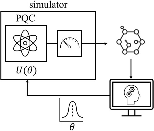
Figure 1. Quantum simulation-based Bayesian inference: A simulator based on a parameterized quantum circuit (PQC) is trained via a likelihood-free Bayesian inference algorithm to serve as a simulator for a physical process of interest.

The motivation for the proposed solution, integrating PQCs with SBI, is twofold. First, from the perspective of SBI, by leveraging quantum circuits as simulators, we follow the well-established principle that quantum computers are best suited for the simulation of certain physical phenomena, especially at the microscopic scale (Georgescu et al., 2014). Second, from the viewpoint of quantum machine learning, Bayesian learning methods have been argued to be potentially beneficial as they can be better account for uncertainty in the model space, enhancing test-time performance (Duffield et al., 2022). Our work thus contributes to the literature on quantum machine learning by moving beyond the likelihood-based method investigated in (Duffield et al., 2022) by leveraging state-of-the-art likelihood-free SBI methods.

1.3 Main contributions

This work explores the application of Bayesian SBI for the training of simulators implemented as PQCs. The main contributions are as follows.

$•$ First, in a tutorial style, the article reviews two families of Bayesian SBI methods, namely, sampling-based and surrogate-based techniques. Sampling-based schemes aim at producing samples from the posterior distribution of the parameters, whilst surrogate-based methods estimate a surrogate for either the likelihood or directly for the posterior distribution in the model parameter space.

$•$ Second, we provide examples via numerical experiments that investigate and compare different circuit architectures for quantum SBI. We specifically investigate the potential gains of encoding inductive biases in the form of symmetry-preserving circuits, following the principles of geometric learning (Ragone et al., 2022). Experimental results indicate that well-motivated quantum circuits that account for the structure of the underlying physical system are capable of simulating data from two distinct tasks.

2 Bayesian simulation-based inference

Let us assume the availability of a data set $\mathcal{D}=\{X_1,X_2,\dots ,X_N\}$, where each data point $X_n\in {\mathbb{R}}^d$ for all $n\in \{\mathrm{1,2},\dots ,N\}$ is modelled as being generated from an unknown ground-truth distribution $p^{*}(X)$. We are interested in optimizing a simulation-based generative model that is able to draw samples approximately distributed according to $p^{*}(X)$.

To this end, we fix a class of parameterized simulators $p(X|\theta )$ that, given a model parameter vector $\theta \in \mathrm{\Theta }\subseteq {\mathbb{R}}^p$, can generate i.i.d. samples $X\sim p(X|\theta )$. Importantly, the value of the probability $p(X|\theta )$ as a function of the model parameter $\theta$, which is known as the likelihood function, is not efficiently computable. Accordingly, models of this type are referred to as being likelihood-free. As we will discuss in the following, this setting describes well the use of parameterized quantum circuits as generative models.

We focus on the problem of inferring the parameter vector $\theta$ of the simulator based on the data set $\mathcal{D}$, which is known as simulation-based inference (SBI). We specifically adopt a Bayesian framework, with the goal of quantifying the epistemic uncertainty on model parameter $\theta$ given limitations on data availability. In this setting, the main quantity of interest is the posterior distribution on the simulator’s parameter’s $\theta$, i.e.,

$p\left(\theta |\mathcal{D}\right)\propto p\left(\theta \right)p\left(\mathcal{D}|\theta \right),(1)$

where $p(\theta )$ is a prior distribution on the model parameter $\theta$, and

$p\left(\mathcal{D}|\theta \right)=\prod _{n=1}^{N}p\left(X_n|\theta \right),(2)$

is the likelihood evaluated on the data set $\mathcal{D}$. With Bayesian SBI, the simulator generates new samples $X$ that are approximately drawn from the marginal distribution

$p\left(X|\mathcal{D}\right)=\int p\left(\theta |\mathcal{D}\right)p\left(X|\theta \right)d\theta (3)$

of data point $X$ given the available data $\mathcal{D}$.

Since the likelihood $p(\mathcal{D}|\theta )$ cannot be evaluated, standard Bayesian inference approaches are not applicable, and one can distinguish two main classes of methods.

$•$ Sampling-based schemes, also known as approximate Bayesian computation (ABC): ABC methods aim at producing samples $\theta \sim p(\theta |\mathcal{D})$ from the posterior distribution (Sunnåker et al., 2013; Beaumont, 2019). These samples can be used to estimate the posterior distribution $p(\theta |\mathcal{D})$ using standard density learning techniques; or directly to draw new samples $X$ that are approximately distributed as the marginal distribution (Equation 3) (Lu and Van Roy, 2017; Qin et al., 2022).

$•$ Surrogate-based schemes: Based on the data set $\mathcal{D}$, surrogate-based methods estimate the likelihood $p(\mathcal{D}|\theta )$, or directly for the posterior $p(\theta |\mathcal{D})$ (Price et al., 2018; Papamakarios et al., 2019; Thomas et al., 2022). In the former case, the (unnormalized) posterior distribution can be estimated by using the definition (Equation 1). Furthermore, samples from the posterior $p(\theta |\mathcal{D})$ or directly from the marginal distribution $p(X|\mathcal{D})$ in (Equation 3) can be produced via Markov chain Monte Carlo techniques (Marjoram et al., 2003; Sisson and Fan, 2010; Brooks et al., 2011).

The rest of the paper is organized as follows. Section 2 presents the problem of Bayesian SBI. Section 3, 4 review Bayesian SBI methods based on sampling and surrogate functions, respectively. Section 5 presents the proposed approach based on quantum simulators. Section 6 presents experimental results, and Section 7 concludes the paper.

3 Bayesian SBI via sampling

In this section, we describe sampling-based Bayesian SBI.

3.1 Model

As shown in Figure 2, sampling-based Bayesian SBI, also known as ABC, models the data-generating mechanism via a hierarchical probability distribution. In it, the simulator $p(\cdot |\theta )$ produces samples $Z$ that are related to the true samples $X$ by a mismatch model. This distribution posits an ancestral sampling procedure, whereby.

1. A model parameter is drawn from the prior $\theta \sim p(\theta )$;

2. The simulator outputs conditionally independent and identically distributed latent variables $\mathcal{Z}=\{Z_1,Z_2,\dots ,Z_M\}$, where $Z_i\in {\mathbb{R}}^d$ for every $i\in \{\mathrm{1,2},\dots ,M\}$, with probability

$p\left(\mathcal{Z}|\theta \right)=\prod _{m=1}^{M}p\left(Z_n|\theta \right);(4)$

3. And the data set $\mathcal{D}$ is generated from the mismatch model $p(\mathcal{D}|\mathcal{Z})$.

Figure 2

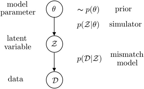
Figure 2. Probabilistic graphical model adopted by sampling-based Bayesian SBI. We follow here the definition of mismatch model given in (Schmon et al., 2020).

The distribution $p(\mathcal{D}|\mathcal{Z})$ defining the mismatch model is subject to design, and it accounts for the fact that the simulator $p(\cdot |\theta )$ is generally misspecified (Schmon et al., 2020). This is in the sense that there is typically no model parameter $\theta$ such that the simulator $p(\cdot |\theta )$ matches exactly the data-generating distribution

$p^{*}\left(\mathcal{D}\right)=\prod _{n=1}^N{p}^{*}\left(X_n\right).(5)$

if no such mismatch is expected, one can set

$p\left(\mathcal{D}|\mathcal{Z}\right)=\mathbb{1}\left(\mathcal{D}=\mathcal{Z}\right),(6)$

where $\mathbb{1}(\cdot )$ is the indicator function for discrete data and the Dirac impulse function for continuous-valued data.

More generally, the choice of the mismatch model must account for requirements of accuracy and efficiency, and it is typically specified as (Wilkinson, 2013; Schmon et al., 2020)

$p\left(\mathcal{D}|\mathcal{Z}\right)\propto \kappa \left(S\left(\mathcal{D}\right),S\left(\mathcal{Z}\right)\right),(7)$

where $\kappa (\cdot ,\cdot )$ is a kernel function and $S(\cdot )\in {\mathbb{R}}^s$ is an $s$-dimensional summary statistic. The choice of the statistics $S(\cdot )$ is often done based on knowledge about the problem. For instance, for discrete-time sequences, one may use as statistics empirical transition rates (Sunnåker et al., 2013).

By (Equation 7), the data $\mathcal{D}$ are assumed to be more likely to correspond to samples $\mathcal{Z}$ if the data sets $\mathcal{D}$ and $\mathcal{Z}$ are “closer” in terms of the correlation between the statistics $S(\mathcal{D})$ and $S(\mathcal{Z})$ as measured by the kernel $\kappa (\cdot ,\cdot )$. A typical choice for the kernel yields (Sunnåker et al., 2013)

$p\left(\mathcal{D}|\mathcal{Z}\right)\propto \mathbb{1}\left(\rho \left(S\left(\mathcal{D}\right),S\left(\mathcal{Z}\right)\right)\le ϵ\right),(8)$

where $\rho (\cdot ,\cdot )$ is an error measure and $ϵ>0$ is tolerance level. Equivalently, the distribution (Equation 7) can be expressed as (Schmon et al., 2020)

$p\left(\mathcal{D}|\mathcal{Z}\right)\propto e^{-\ell \left(S\left(\mathcal{D}\right),S\left(\mathcal{Z}\right)\right)},(9)$

where $\ell (\cdot ,\cdot )$ is a loss function measuring the discrepancy between the statistics $S(\mathcal{D})$ and $S(\mathcal{Z})$. Specifically, to match (Equation 7), one can set the loss as $\ell (S,S^{\prime })=-\log (\kappa (S,S^{\prime }))$.

By the model in Figure 2, the posterior distribution over model parameters and samples produced by the simulator given the data set $\mathcal{D}$ is given by

$p\left(\theta ,\mathcal{Z}|\mathcal{D}\right)\propto p\left(\theta \right)p\left(\mathcal{Z}|\theta \right)p\left(\mathcal{D}|\mathcal{Z}\right).(10)$

by marginalizing out the simulator’s outputs $\mathcal{Z}$, we obtain the model parameter posterior as

$p\left(\theta |\mathcal{D}\right)=\int p\left(\theta ,\mathcal{Z}|\mathcal{D}\right)d\mathcal{Z}.(11)$

in the special case in which no mismatch is accounted for in the model, i.e., when $p(\mathcal{D}|\mathcal{Z})=\mathbb{1}(\mathcal{Z}=\mathcal{D})$, then the distribution (Equation 11) evaluates as

$p\left(\theta |\mathcal{D}\right)=p\left(\theta ,\mathcal{Z}=\mathcal{D}|\mathcal{D}\right)\propto p\left(\theta \right)p\left(\mathcal{D}|\theta \right),(12)$

which corresponds to the conventional posterior distribution (Equation 1) in the ideal case of a well-specified model.

The goal of ABC is to produce samples $\theta$ of the model parameter vector that are approximately distributed according to the posterior distribution $p(\theta |\mathcal{D})$ in (Equation 11). This can be accomplished by generating samples $(\theta ,\mathcal{Z})$ from the joint posterior $p(\theta ,\mathcal{Z}|\mathcal{D})$ in (Equation 10), and then discarding the simulator’s outputs $\mathcal{Z}$. We next review two ABC methods of increasing complexity and efficacy.

3.2 Rejection-sampling ABC

Rejection-sampling ABC (RS-ABC) iteratively draws candidate samples ${\theta }^{\prime }$ from the prior $p(\theta )$. Each such sample is accepted with a probability that ensures that all accepted samples are drawn from the posterior $p(\theta |\mathcal{D})$ (Beaumont et al., 2002; Sunnåker et al., 2013).

To this end, for each candidate model parameter sample ${\theta }^{\prime }$, the simulator produces $M$ samples ${\mathcal{Z}}^{\prime }=\{Z_1^{\prime },Z_2^{\prime },\dots ,Z_M^{\prime }\}$ distributed as $p(\mathcal{Z}|\theta )={\prod }_{m=1}^{M}p(Z_m^{\prime }|{\theta }^{\prime })$. Therefore, RS-ABC produces the candidate pair $({\theta }^{\prime },{\mathcal{Z}}^{\prime })$ distributed as

$\left({\theta }^{\prime },{\mathcal{Z}}^{\prime }\right)\sim p\left(\theta \right)\prod _{m=1}^{M}p\left(Z_m^{\prime }|{\theta }^{\prime }\right).(13)$

The sample $({\theta }^{\prime },{\mathcal{Z}}^{\prime })$ is selected with acceptance probability $p(\mathrm{a}\mathrm{c}\mathrm{c}|{\theta }^{\prime },{\mathcal{Z}}^{\prime })$, where “$\mathrm{a}\mathrm{c}\mathrm{c}$” denotes the event that a candidate sample is accepted. The acceptance probability generally depends on the model parameter ${\theta }^{\prime }$ and on the generated samples ${\mathcal{Z}}^{\prime }$, as discussed next.

The distribution of an accepted sample can be computed as

$p\left(\theta ,\mathcal{Z}|\mathrm{a}\mathrm{c}\mathrm{c}\right)\propto p\left(\theta \right)p\left(\mathcal{Z}|\theta \right)p\left(\mathrm{a}\mathrm{c}\mathrm{c}|\theta ,\mathcal{Z}\right).(14)$

Therefore, in order for the distribution (Equation 14) to match the desired posterior (Equation 10), one can set

$p\left(\mathrm{a}\mathrm{c}\mathrm{c}|\theta ,\mathcal{Z}\right)\propto p\left(\mathcal{D}|\mathcal{Z}\right).(15)$

In particular, if $p(\mathcal{D}|\mathcal{Z})$ is selected as per the conventional choice in (Equation 8), then the acceptance step is simplified as

$\text{accept\hspace{0.17em}candidate\hspace{0.17em}sample\hspace{0.17em}}\left({\theta }^{\prime },{\mathcal{Z}}^{\prime }\right)\text{if}\rho \left(S\left(\mathcal{D}\right),S\left(Z^{\prime }\right)\right)\le ϵ.(16)$

3.3 Metropolis-Hastings ABC

RS-ABC typically produces a low rate of acceptance of the generated samples, particularly when data are sufficiently high dimensional. To see this, consider the common case in which the prior $p(\theta )$ supports, with non-negligible probability, model parameters $\theta$ corresponding to simulators $p(\cdot |\theta )$ that are very different from the ground-truth distribution $p^{*}(\cdot )$. Using the conventional acceptance rule (Equation 16), a sample $({\theta }^{\prime },{\mathcal{Z}}^{\prime })$ is retained only if the sufficient statistics $S(\mathcal{D})$ and $S({\mathcal{Z}}^{\prime })$ for simulator’s samples and data set are sufficiently close. Given that RS-ABC draws the model parameter $\theta$ from the prior as per (3.2), this acceptance event is quite unlikely, resulting in a low rate of acceptance of the generated samples.

To overcome this drawback, reference (Marjoram et al., 2003) proposed Metropolis-Hastings ABC (MH-ABC). MH-ABC proceeds to sample from Equation 10) in a sequential manner. To elaborate, let us denote as ${\theta }_{i-1}$ the last sample accepted at the beginning of the $i$-th iteration. Furthermore, we introduce a transition probability distribution $q(\cdot |{\theta }_{i-1})$, which constitute a key design choice for MH-ABC. At the $i$-th iteration, a new sample $({\theta }^{\prime },{\mathcal{Z}}^{\prime })$ is drawn from the conditional proposal distribution

$q\left({\theta }^{\prime },{\mathcal{Z}}^{\prime }|{\theta }_{i-1}\right)=q\left({\theta }^{\prime }|{\theta }_{i-1}\right)p\left({\mathcal{Z}}^{\prime }|{\theta }^{\prime }\right).(17)$

accordingly, a new parameter ${\theta }^{\prime }$ is sampled from the Markov transition kernel $q(\cdot |{\theta }_{i-1})$ dependent on the last accepted sample ${\theta }_{i-1}$, and the data set ${\mathcal{Z}}^{\prime }$ is generated from the simulator $p(\cdot |{\theta }^{\prime })$. The rationale for this choice is that samples close to previously accepted samples, as dictated by the distribution $q(\cdot |{\theta }_{i-1})$ may be more likely to have the desired distribution. The downside of the approach is that consecutive accepted samples are not independent, as in RS-ABC. Rather, the temporal correlation is determined by the Markov kernel $q(\cdot |{\theta }_{i-1})$.

Let $p(\mathrm{a}\mathrm{c}\mathrm{c}|{\theta }^{\prime },{\mathcal{Z}}^{\prime })$ be the acceptance probability of the proposed sample $({\theta }^{\prime },{\mathcal{Z}}^{\prime })$. In order to ensure a stationary distribution given by the posterior $p(\theta ,\mathcal{Z}|\mathcal{D})$, it is sufficient to impose detailed-balance condition (Hastings, 1970)

$p\left({\theta }_{i-1},{\mathcal{Z}}_{i-1}|\mathcal{D}\right)q\left({\theta }^{\prime },{\mathcal{Z}}^{\prime }|{\theta }_{i-1}\right)p\left(\mathrm{a}\mathrm{c}\mathrm{c}|{\theta }^{\prime },{\mathcal{Z}}^{\prime }\right)=p\left({\theta }^{\prime },{\mathcal{Z}}^{\prime }|\mathcal{D}\right)q\left({\theta }_{i-1},{\mathcal{Z}}_{i-1}|{\theta }^{\prime }\right)p\left(\mathrm{a}\mathrm{c}\mathrm{c}|{\theta }_{i-1},{\mathcal{Z}}_{i-1}\right).(18)$

this equality can be ensured by setting

$p\left(\mathrm{a}\mathrm{c}\mathrm{c}|{\theta }^{\prime },{\mathcal{Z}}^{\prime }\right)=\min \left(1,\frac{p\left({\theta }^{\prime },{\mathcal{Z}}^{\prime }|\mathcal{D}\right)}{p\left({\theta }_{i-1},{\mathcal{Z}}_{i-1}|\mathcal{D}\right)}\cdot \frac{q\left({\theta }_{i-1},{\mathcal{Z}}_{i-1}|{\theta }^{\prime }\right)}{q\left({\theta }^{\prime },{\mathcal{Z}}^{\prime }|{\theta }_{i-1}\right)}\right).(19)$

using Equations 10, 17, we finally get the acceptance probability adopted by MH-ABC as

$\begin{array}{ll}\hfill p\left(\mathrm{a}\mathrm{c}\mathrm{c}|{\theta }^{\prime },{\mathcal{Z}}^{\prime }\right)& =\min \left(1,\frac{p\left({\theta }^{\prime }\right)p\left({\mathcal{Z}}^{\prime }|{\theta }^{\prime }\right)p\left(\mathcal{D}|{\mathcal{Z}}^{\prime }\right)}{p\left({\theta }_{i-1}\right)p\left({\mathcal{Z}}_{i-1}|{\theta }_{i-1}\right)p\left(\mathcal{D}|{\mathcal{Z}}_{i-1}\right)}\cdot \frac{q\left({\theta }_{i-1}|{\theta }^{\prime }\right)p\left({\mathcal{Z}}_{i-1}|{\theta }_{i-1}\right)}{q\left({\theta }^{\prime }|{\theta }_{i-1}\right)p\left({\mathcal{Z}}^{\prime }|{\theta }^{\prime }\right)})\right)\hfill \\ \hfill & =\min \left(1,\frac{p\left({\theta }^{\prime }\right)p\left(\mathcal{D}|{\mathcal{Z}}^{\prime }\right)}{p\left({\theta }_{i-1}\right)p\left(\mathcal{D}|{\mathcal{Z}}_{i-1}\right)}\cdot \frac{q\left({\theta }_{i-1}|{\theta }^{\prime }\right)}{q\left({\theta }^{\prime }|{\theta }_{i-1}\right)}\right).\hfill \end{array}(20)$

4 Bayesian SBI via surrogates

Unlike sampling-based methods, surrogate-based methods use the simulator, along with the data set $\mathcal{D}$, to estimate the likelihood $p(\mathcal{D}|\theta )$, or directly the posterior $p(\theta |\mathcal{D})$. To this end, surrogate-based techniques do not explicitly model the mismatch between simulator and ground-truth data-generation mechanism as done by sampling-based methods (see Figure 2). Rather, they directly use the data generation mechanism as the generative model $p(\theta ,\mathcal{D})=p(\theta )p(\mathcal{D}|\theta )$, with the simulator-based data likelihood given by $p(\mathcal{D}|\theta )={\prod }_{n=1}^{N}p(X_n|\theta )$. Accordingly, in this section, we use the notation $X$ for the samples generated by the simulator. Next, we review state-of-the-art methods based on ratio estimation.

4.1 Ratio estimation

Ratio estimation (RE) applies contrastive learning to estimate the ratio between the likelihood $p(\mathcal{D}|\theta )$, which is not available in the likelihood-free setting of interest, and the data marginal $p(\mathcal{D})$, i.e. (Thomas et al., 2022),

$r\left(\mathcal{D},\theta \right)=\frac{p\left(\mathcal{D}|\theta \right)}{p\left(\mathcal{D}\right)}.(21)$

given an estimate $\widehat{r}(\mathcal{D},\theta )$ of the ratio, the likelihood can be in principle estimated as $\widehat{p}(\mathcal{D}|\theta )\propto \widehat{r}(\mathcal{D},\theta )$, and the posterior distribution as

$\widehat{p}\left(\theta |\mathcal{D}\right)\propto p\left(\theta \right)\widehat{p}\left(\mathcal{D}|\theta \right).(22)$

In practice, the unnormalized posterior in (Equation 22) can be used, without the need for an explicit normalization, to obtain samples $\theta \sim \widehat{p}(\theta |\mathcal{D})$ with the aid of Markov chain Monte Carlo (MCMC) techniques (Cranmer et al., 2020; Simeone, 2022).

RE methods train a binary classifier to distinguish between data sets generated according to the distributions at the numerator and denominator of the ratio (Equation 21). To this end, for any fixed value $\theta$, the simulator is first leveraged to generate two classes of data sets, with each data set containing a number $N$ of examples. The first class of data sets contains data sets $\mathcal{X}$ drawn according to the distribution $p(\mathcal{X}|\theta )={\prod }_{m=1}^{M}p(X_m|\theta )$; while the second class contains data sets drawn from the marginal $p(\mathcal{X})=\int p(\mathcal{X}|\theta )p(\theta )d\theta$.

To generate data sets in the first class, one directly runs the simulator with the given value $\theta$. For the second class, one first samples ${\theta }^{\prime }\sim p(\theta )$ from the prior, and then a data set $\mathcal{X}={\{X_m\sim p(X|{\theta }^{\prime })\}}_{m=1}^M$, discarding the sample ${\theta }^{\prime }$. We assign label $t=1$ to all data sets in the first class, and the label $t=0$ to all data sets in the second class.

The binary classifier takes as input a data set $\mathcal{X}$ of $M$ examples, computes a fixed function $S(\mathcal{X})$, and outputs a probability distribution $p(t|S(\mathcal{X}),\varphi )$ quantifying the confidence of the predictor in $\mathcal{X}$ belonging to either class. The classifier depends on a model parameter vector $\varphi$. If the classifier is well trained, the probability $p(t|S(\mathcal{X}),\varphi )$ provides a good approximation of the true posterior distribution $p(t|S(\mathcal{X}))$, as discussed next.

By the construction of the data set, a data set $\mathcal{X}$ is conditionally distributed as.

$p\left(\mathcal{X}|t=1\right)=p\left(\mathcal{X}|\theta \right)(23)$

$p\left(\mathcal{X}|t=0\right)=p\left(\mathcal{X}\right).(24)$

furthermore, the posterior distribution is

$\begin{array}{ll}\hfill p\left(t=1|\mathcal{X}\right)& =\frac{p\left(t=1\right)p\left(\mathcal{X}|t=1\right)}{p\left(t=0\right)p\left(\mathcal{X}|t=0\right)+p\left(t=1\right)p\left(\mathcal{X}|t=1\right)}\hfill \\ \hfill & =\frac{p\left(t=1\right)p\left(\mathcal{X}|\theta \right)}{p\left(t=0\right)p\left(\mathcal{X}\right)+p\left(t=1\right)p\left(\mathcal{X}|\theta \right)}.\hfill \end{array}(25)$

writing $p(t=1)/p(t=0)=\alpha$ we get

$p\left(t=1|\mathcal{X}\right)=\frac{\alpha p\left(\mathcal{X}|\theta \right)}{p\left(\mathcal{X}\right)+\alpha p\left(\mathcal{X}|\theta \right)}(26)$

and

$p\left(t=0|\mathcal{X}\right)=1-p\left(t=1|\mathcal{X}\right)=\frac{p\left(\mathcal{X}\right)}{p\left(\mathcal{X}\right)+\alpha p\left(\mathcal{X}|\theta \right)}.(27)$

Making the approximation $p(t|S(\mathcal{X}),\varphi )\approx p(t|\mathcal{X})$, we can finally estimate the ratio of likelihood and data marginal as

$\widehat{r}\left(\mathcal{D},\theta \right)\approx \frac{p\left(t=1|S\left(\mathcal{D}\right),\varphi \right)}{p\left(t=0|S\left(\mathcal{D}\right),\varphi \right)}.(28)$

4.2 Amortized ratio estimation

To improve the performance of RE, amortization techniques can be used, whereby the classifier is amortized using the parameters from the simulator. To explain, note that the true ratio can be equivalently expressed as

$r\left(\mathcal{D},\theta \right)=\frac{p\left(\mathcal{X}|\theta \right)}{p\left(\mathcal{X}\right)}=\frac{p\left(\mathcal{X},\theta \right)}{p\left(\mathcal{X}\right)p\left(\theta \right)}.(29)$

This modification suggests a way to train the binary classifier to distinguish between dependent sample-parameter pairs $(\mathcal{X},\theta )\sim p(\mathcal{X},\theta )$, which are assigned class label $t=1$, from independent sample-parameter pairs $(\mathcal{X},\theta )\sim p(\mathcal{X})p(\theta )$, which are assigned class label $t=0$. To do so, samples from the first class are generated by running the simulator with the given value $\theta$, and concatenating the sampled sequence to the vector $\theta$. For the second class, one again first samples ${\theta }^{\prime }\sim p(\theta )$ from the prior along with a data set $\mathcal{X}={\{X_m\sim p(X|{\theta }^{\prime })\}}_{m=1}^M$, discarding the sample ${\theta }^{\prime }$; and then generates new, independent, ${\theta }^{\prime }\sim p(\theta )$ to which one concatenates the output of the simulator. This method is referred to as amortized RE (Hermans et al., 2020).

In cases when the divergence between the densities is large, the classifier can obtain almost perfect accuracy with a relatively poor estimate of the density ratio. This failure mode is known as the density-chasm problem, and can be overcome by transporting samples from one distribution to the other, creating a chain of intermediate data sets. The density-ratio between consecutive datasets along this chain can be then accurately estimated via classification. The chained ratios are then combined via a telescoping product to obtain an estimate of the original density-ratio. This method is referred to as telescopic amortized RE (Montel et al., 2023).

Finally, as practical note, we emphasize that, both in the amortized and non-amortized settings, to avoid numerical errors one can extract the logit, $\log (\widehat{r}(\mathcal{D},\theta ))$, from the classifier before applying the activation in the output layer. This choice also mitigates vanishing gradient issues.

5 Quantum bayesian simulation-based inference

In the previous sections, we have reviewed sampling-based and surrogate-based Bayesian SBI techniques. In the proposed quantum Bayesian SBI system, illustrated in Figure 1, both classes of methods are applicable. The key new element is the introduction of a PQC as the simulator $p(X|\theta )$ (or $p(Z|\theta )$ in the notation of Section 3).

5.1 Parameterized quantum circuits as simulators

The proposed quantum SBI solution aims at developing simulators for the generation of a quantity of interest $X$ that can take values in a set of $2^d$ elements for some integer $d$. Note that this requires the quantity $X$ to be either discrete to start with, or to be quantized as finely as allowed by a resolution of $d$ bits. To this end, we propose to implement a PQC that acts on a register of $d$ qubits. Accordingly, the allowed resolution of quantity $X$ increases exponentially with the physical dimension of the qubit register. In such a setting, one can assume, without loss of generality, that the quantity $X$ – or its quantized version–assumes values in the set of integers $\{\mathrm{0,1},\dots ,2^d-1\}$, or equivalently in the set of all binary strings of $d$ bits.

As reviewed in (Schuld and Petruccione, 2021; Simeone et al., 2022), PQCs implement a parameterized unitary transformation $U(\theta )$, a $2^d\times 2^d$ complex-valued matrix, on a register of a given number, $d$, of qubits. The unitary transformation $U(\theta )$ is described by a quantum circuit that is specified by quantum gates placed according to a predefined arrangement. The arrangement is referred to as the ansatz of the PQC. Some of the quantum gates in the quantum circuit can be controlled by selecting real-valued parameters, which are collectively denoted as vector $\theta$, see Figure 3.

Figure 3

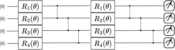
Figure 3. An example of a PQC which serves as a simulator of a physical process. In this work, we propose to treat the PQC as a likelihood-free model that can be trained via Bayesian simulation-based inference.

Initializing the register of $d$ qubits in a reference state $|{0\rangle }^{\otimes d}$, the PQC produces the output state

$|\psi \left(\theta \right)\rangle =U\left(\theta \right)|{0\rangle }^{\otimes d}.(30)$

Furthermore, by Born’s rule, the probability distribution $p(X|\theta )$ is given by

$p\left(X|\theta \right)=|⟨X|\psi \left(\theta \right)⟩{|}^2,(31)$

where $|X\rangle$ represents the state in the computational basis corresponding to integer $X$.

5.2 Choosing the ansatz

In general, choosing a good ansatz for the quantum simulator entails a difficult trade-off between adherence to the physics of the problem and complexity of implementation. In particular, if prior knowledge about the structure of the data are available, this may be encoded as an inductive bias into the choice of the quantum circuit architecture, assuming that the complexity of the implementation allows it.

The typical way to encode structure into the ansatz is to leverage symmetries in the data. Symmetries refer to transformations of the data that leave it invariant or change it in a predictable, equivariant manner. For example, the binding energy of a molecule does not change by permuting the order of the atoms, and a picture of a cat still depicts a cat regardless of the position of the cat within the image. This prior knowledge can be encoded into the simulator ansatz as a geometric prior. Notable examples include quantum graph neural networks (QGNNs) (Verdon et al., 2019; Mernyei et al., 2022) and quantum convolutional neural network (QCNNs) (Cong et al., 2019), which preserve equivariance to permutations and shifts, respectively. Other examples include quantum recurrent neural networks for time series processing (Nikoloska et al., 2023).

In the absence of prior knowledge, or when the practitioner is concerned with efficient hardware implementation, they may choose to use a hardware-efficient architecture (HEA). Such architectures use only single qubit and two qubit gates, placed along the existing connectivity of the quantum computer, which are easily implemented on both gate-based or pulse-based NISQ machines (Zulehner et al., 2018; Gyongyosi and Imre, 2021).

6 Results

In this section, we provide experimental results to validate the proposed concept of quantum Bayesian SBI.

6.1 Tasks

6.1.1 Generating bars-and-stripes images

We first consider the classical small-scale benchmark problem of generating $2\times 2$ images from the bars-and-stripes (BAS) data set MacKay and Mac Kay, 2003. BAS is a synthetic data set consisting of four images. Each image consists of a $2\times 2$ grid of black, denoted as $“1^{″}$, and white, denoted as $“0^{″}$, pixels. In vector form, bars correspond to bit strings $X$ of the form $[0011]$ and $[1100]$, while stripes correspond to bit strings $[0101]$ and $[1010]$.

6.1.2 Simulating molecular topologies

In this second task, which is closer to a real-life application of the proposed method, the task of the simulator is to generate valid molecular structures, i.e., valid primary topologies, for 4-atom molecules comprised of carbon (C), hydrogen (H), boron (B), oxygen (O), or nitrogen (N) atoms. Knowing a valid molecular topology, specifying which atom is covalently bonded to which other atom, is crucial for determining classical potentials for biomolecules. Each sample consists of a $4\times 4$ adjacency matrix describing the covalent bonds in the molecular graph, where $“1^{″}$ denotes the presence of a covalent bond between two atoms, and $“0^{″}$, denotes the absence of a covalent bond. We only consider single covalent bonds, and we use Pennylane datasets (Bergholm et al., 2018), whereby the number of valid structures is 2, whilst the number of all possible structures is 24. In vector form (the upper right adjacency matrix), the topologies of molecules with three H atoms, BH3 and NH3, correspond to bit string $X=[010101]$, whilst the topologies of molecules with two H atoms C2H2, H2O2, N2H2, and H4 correspond to bit string $X=[100101]$.

6.2 Simulator ansatz and hyperparameters

We consider four circuit architectures. All of the considered architectures are comprised of four qubits and two layers.

6.2.1 QCNN

For BAS, an image dataset, we employ a QCNN. QCNN is a translation-equivariant model that uses convolution layers and applies a single quasi-local unitary (Cong et al., 2019). Each pixel is represented by a qubit. We do not employ pooling, and the quasi-local unitary is applied on pairs of qubits. To determine the $i$-th pixel value, we measure the observable $Z_i$.

6.2.2 QGNN

For molecular topologies, we employ a QGNN. as molecules can be well represented as graphs. A QGNN is an permutation-equivariant ansatz (Verdon et al., 2019). Each atom is represented by a qubit. To determine whether a covalent bond is present between each atom pair $(i,j)$, we measure the observable $Z_i{Z}_j$. It is useful to note that, unlike classical graph structure discovery schemes in which the number of trainable parameters scales with the number of edges, in the QGNN architecture, the number of parameters scales with the number of nodes (which is typically much smaller.

6.2.3 HEA

As a basic benchmark, for both tasks, we also implement an HEA, which consists of general single qubit gates, i.e., rotations described by three angles, and by CNOT gates applied in a cyclical manner across all pairs successive qubits. The same observables described above are considered to extract information from the output states for the two tasks.

6.2.4 Separable circuits

Finally, to gauge the potential benefits of entanglement, we adopt a mean-field, or separable, ansatz that consists solely of general single-qubit gates. The resulting circuits can be efficiently simulated on classical computers for any number of qubits, with no need for quantum hardware. Therefore, this setup essentially represents a classical benchmark. The same observables are again applied for the two tasks.

6.3 SBI algorithms

As a representative of sampling-based schemes, we implement RS-SBI with the classical kernel (Equation 8) with summary statistics given by the histogram of the generated samples $\mathcal{Z}$. We set $ϵ=0.3$, and we draw $M=1000$ examples for each draw from the prior distribution $p(\theta )$. For surrogate-based schemes, we adopt the amortized RE technique whereby the surrogate model is implemented as three-member ensemble in which each member is comprised of a transformer layer with three attention heads followed by a linear layer with ReLU activations (Vaswani et al., 2017). The outputs of the ensemble members are averaged to obtain the logit. We use dropout with rate 0.1, and the Adam optimiser with learning rate 0.001.

6.4 Evaluation and performance metrics

We are interested in evaluating the adherence of the distribution of the samples produced by the simulator to the ground-truth data-generating distribution. To this end, for any fixed simulator parameters $\theta$, we use the simulator to generate a large number of samples, namely, 1,000, from the corresponding model distribution $p(X|\theta )$. The probability distribution $p(X|\theta )$ is estimated using the histogram of the generated samples. The quality of the samples is then quantified via the total variation distance (TVD) $D(p(X|\theta ),p^{*}(X))$, where $p^{*}(X)$ is the ground-truth distribution, which in the examples at hand can be obtained from the training set.

In Bayesian SBI, the model parameter $\theta$ is drawn from the learnt posterior distribution, which represents the uncertainty of the learner on the optimal parameters of the simulator. In the examples at hand, the training data sets are sufficiently informative to fully describe the data-generating distribution $p^{*}(X)$. However, epistemic uncertainty remains, owing to the unknown likelihood. In fact, the lack of access to the likelihood limits the information that the learning algorithm can extract from the simulator to the $M$ samples drawn to evaluate the statistics $S(\cdot )$, here the histogram.

Each draw of the model parameter vector $\theta$ yields a generally different TVD $D(p(X|\theta ),p^{*}(X))$ between the distribution produced by the simulator, $p(X|\theta )$, and the ground-truth distribution, $p^{*}(X)$. In the following, we evaluate the epistemic uncertainty produced by Bayesian SBI by plotting an estimate of the distribution of the TVD produced due to the randomness on the model parameter vector $\theta$. The estimate is obtained via a kernel density estimator (KDE) with bandwidth equal to 0.9.

As a benchmark learning algorithm, we also show the performance of a scheme that produces a point estimate for the parameters $\theta$. This strategy may be considered as a representative of frequentist learning methods that do not attempt to characterize epistemic uncertainty. Specifically, we implement a simple approach that looks for the value of parameters $\theta$ that maximizes the likelihood estimated via the TVD between the histogram of the $M$ samples generated by the simulator and the ground-truth distribution. To this end, we retain the parameter vector $\theta$ that yields the minimum mentioned TVD across all samples $\theta$ generated by the considered Bayesian SBI schemes.

6.5 Results

The distributions of the TVD for both sampling- and surrogate-based Bayesian SBI schemes are shown in Figure 4 for the two tasks under study. For this figure, we adopt the best-performing ansatz for each task, namely, the QCNN and QGNN, respectively. It is observed that, by accounting for the uncertainty on the likelihood, Bayesian SBI schemes can outperform conventional frequentist techniques. In fact, samples produced from the posterior distribution can yield significantly lower TVD values, which indicate a closer match of the ground-truth distribution. Furthermore, the spread of the distribution produced by Bayesian SBI strategies is task-dependent. Similarly, the choice between sampling-based and surrogate-based schemes is also seen to depend on the task, with the latter having a clear advantage in the BAS task.

Figure 4

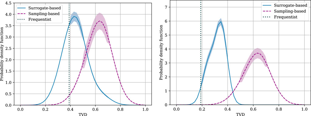
Figure 4. Distribution of the TVD between distribution of the samples produced by the simulator and ground-truth distribution for the BAS data set (left), and for the primary molecular structure task (right).

We now analyze the impact of different ansatzes by showing in Figure 5 distributions of the TVD for various architectures of the quantum simulator. Whilst we do not claim that quantum circuits are provably better than classical counterparts for the problem at hand, the separable circuits is observed to result in a very large TVD. In contrast, for both tasks, the symmetry-preserving simulators–QCNN for the BAS task and QGNN for the molecular topology task–result in the smallest TVD between the generated samples and the true distribution, suggesting that encoding inductive-biases in the simulator is indeed helpful for SBI.

Figure 5

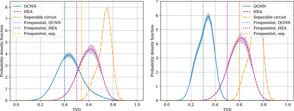
Figure 5. Distribution of the TVD between distribution of the samples produced by the simulator and ground-truth distribution for the BAS data set (left), and for the primary molecular structure task (right).

7 Concluding remarks

Simulation intelligence is an emerging multi-disciplinary topic that views simulation as a central tool for design and discovery (Lavin et al., 2021). The scope and reach of the field are only expected to grow in importance with the fast development of generative artificial intelligence tools and with the spread of digital twinning as a framework for engineering complex systems (Ruah et al., 2023). Quantum circuits are known to be efficient solutions to implementing samplers from complex distributions in discrete spaces. This property makes quantum circuit appealing as co-processors for the controlled generation of latent random variables (Nikoloska and Simeone, 2022). In this context, this work has taken a few steps towards the idea of integrating quantum circuits as simulators in a simulation-based process.

The main aim of this article is to provide readers with a background in quantum machine learning with an introduction to Bayesian SBI tools. Many problems are left open to future investigations, including the investigation of larger-scale use cases, the implementation on NISQ computers, and the analysis of the impact of quantum noise.

Data availability statement

The original contributions presented in the study are included in the article/supplementary material, further inquiries can be directed to the corresponding author.

Author contributions

IN: Data curation, Investigation, Software, Validation, Visualization, Writing–original draft, Writing–review and editing. OS: Conceptualization, Funding acquisition, Methodology, Project administration, Resources, Supervision, Writing–original draft, Writing–review and editing.

Funding

The author(s) declare that financial support was received for the research, authorship, and/or publication of this article. The work of OS was partially supported by the European Union’s Horizon Europe project CENTRIC (101096379), by the Open Fellowships of the EPSRC (EP/W024101/1), by the EPSRC project (EP/X011852/1), and by the United Kingdom Government under Project REASON.

Acknowledgments

The authors acknowledge the contribution of Hari Hara Suthan Chittoor in the early stages of this study.

Conflict of interest

The authors declare that the research was conducted in the absence of any commercial or financial relationships that could be construed as a potential conflict of interest.

Publisher’s note

All claims expressed in this article are solely those of the authors and do not necessarily represent those of their affiliated organizations, or those of the publisher, the editors and the reviewers. Any product that may be evaluated in this article, or claim that may be made by its manufacturer, is not guaranteed or endorsed by the publisher.

References

Beaumont, M. A. (2019). Approximate Bayesian computation. Annu. Rev. Statistics Its Appl. 6, 379–403. doi:10.1146/annurev-statistics-030718-105212

CrossRef Full Text | Google Scholar

Beaumont, M. A., Zhang, W., and Balding, D. J. (2002). Approximate Bayesian computation in population genetics. Genetics 162, 2025–2035. doi:10.1093/genetics/162.4.2025

PubMed Abstract | CrossRef Full Text | Google Scholar

Bergholm, V., Izaac, J., Schuld, M., Gogolin, C., Ahmed, S., Ajith, V., et al. (2018). Pennylane: automatic differentiation of hybrid quantum-classical computations. arXiv Prepr. arXiv:1811.04968.

Google Scholar

Brooks, S., Gelman, A., Jones, G., and Meng, X. L. (2011). Handbook of Markov chain Monte Carlo. United Kingdom: CRC Press.

Google Scholar

Cong, I., Choi, S., and Lukin, M. D. (2019). Quantum convolutional neural networks. Nat. Phys. 15, 1273–1278. doi:10.1038/s41567-019-0648-8

CrossRef Full Text | Google Scholar

Cranmer, K., Brehmer, J., and Louppe, G. (2020). The frontier of simulation-based inference. Proc. Natl. Acad. Sci. 117, 30055–30062. doi:10.1073/pnas.1912789117

PubMed Abstract | CrossRef Full Text | Google Scholar

Dada, J. O., and Mendes, P. (2011). Multi-scale modelling and simulation in systems biology. Integr. Biol. 3, 86–96. doi:10.1039/c0ib00075b

PubMed Abstract | CrossRef Full Text | Google Scholar

Duffield, S., Benedetti, M., and Rosenkranz, M. (2022). Bayesian learning of parameterised quantum circuits. arXiv Prepr. arXiv:2206.07559.

Google Scholar

Elshafei, Y., Tonts, M., Sivapalan, M., and Hipsey, M. (2016). Sensitivity of emergent sociohydrologic dynamics to internal system properties and external sociopolitical factors: implications for water management. Water Resour. Res. 52, 4944–4966. doi:10.1002/2015wr017944

CrossRef Full Text | Google Scholar

Georgescu, I. M., Ashhab, S., and Nori, F. (2014). Quantum simulation. Rev. Mod. Phys. 86, 153–185. doi:10.1103/revmodphys.86.153

CrossRef Full Text | Google Scholar

Gyongyosi, L., and Imre, S. (2021). Scalable distributed gate-model quantum computers. Sci. Rep. 11, 5172. doi:10.1038/s41598-020-76728-5

PubMed Abstract | CrossRef Full Text | Google Scholar

Hastings, W. K. (1970). Monte Carlo sampling methods using Markov chains and their applications. Biometrika 57, 97–109. doi:10.1093/biomet/57.1.97

CrossRef Full Text | Google Scholar

Hermans, J., Begy, V., and Louppe, G. (2020). “Likelihood-free mcmc with amortized approximate ratio estimators,” in International conference on machine learning. United Kingdom: PMLR, 4239–4248.

Google Scholar

Lavin, A., Krakauer, D., Zenil, H., Gottschlich, J., Mattson, T., Brehmer, J., et al. (2021). Simulation intelligence: towards a new generation of scientific methods. arXiv Prepr. arXiv:2112.03235.

Google Scholar

Lu, X., and Van Roy, B. (2017). Ensemble sampling. Adv. neural Inf. Process. Syst. 30.

Google Scholar

MacKay, D. J., and Mac Kay, D. J. (2003). Information theory, inference and learning algorithms. United Kingdom: Cambridge University Press.

Google Scholar

Marjoram, P., Molitor, J., Plagnol, V., and Tavaré, S. (2003). Markov chain Monte Carlo without likelihoods. Proc. Natl. Acad. Sci. 100, 15324–15328. doi:10.1073/pnas.0306899100

PubMed Abstract | CrossRef Full Text | Google Scholar

Mernyei, P., Meichanetzidis, K., and Ceylan, I. I. (2022). “Equivariant quantum graph circuits,” in International conference on machine learning. United Kingdom: PMLR, 15401–15420.

Google Scholar

Montel, N. A., Alvey, J., and Weniger, C. (2023). Scalable inference with autoregressive neural ratio estimation. arXiv Prepr. arXiv:2308.08597.

Google Scholar

Nikoloska, I., and Simeone, O. (2022). “Quantum-aided meta-learning for Bayesian binary neural networks via born machines,” in 2022 IEEE 32nd international Workshop on machine Learning for signal processing (MLSP) (IEEE), 1–6.

CrossRef Full Text | Google Scholar

Nikoloska, I., Simeone, O., Banchi, L., and Veličković, P. (2023). Time-warping invariant quantum recurrent neural networks via quantum-classical adaptive gating. Mach. Learn. Sci. Technol. 4, 045038. doi:10.1088/2632-2153/acff39

CrossRef Full Text | Google Scholar

Papamakarios, G., Sterratt, D., and Murray, I. (2019). “Sequential neural likelihood: fast likelihood-free inference with autoregressive flows,” in The 22nd international Conference on artificial Intelligence and statistics (PMLR), 837–848.

Google Scholar

Price, L. F., Drovandi, C. C., Lee, A., and Nott, D. J. (2018). Bayesian synthetic likelihood. J. Comput. Graph. Statistics 27, 1–11. doi:10.1080/10618600.2017.1302882

CrossRef Full Text | Google Scholar

Qin, C., Wen, Z., Lu, X., and Van Roy, B. (2022). An analysis of ensemble sampling. arXiv Prepr. arXiv:2203.01303.

Google Scholar

Ragone, M., Braccia, P., Nguyen, Q. T., Schatzki, L., Coles, P. J., Sauvage, F., et al. (2022). Representation theory for geometric quantum machine learning. arXiv Prepr. arXiv:2210.07980.

Google Scholar

Ruah, C., Simeone, O., and Al-Hashimi, B. (2023). A Bayesian framework for digital twin-based control, monitoring, and data collection in wireless systems. IEEE J. Sel. Areas Commun. 41, 3146–3160. doi:10.1109/jsac.2023.3310093

CrossRef Full Text | Google Scholar

Schmon, S. M., Cannon, P. W., and Knoblauch, J. (2020). Generalized posteriors in approximate Bayesian computation. arXiv preprint arXiv:2011.08644.

Google Scholar

Schuld, M., and Petruccione, F. (2021). Machine learning with quantum computers. Springer.

Google Scholar

Simeone, O. (2022). Machine learning for engineers. Cambridge University Press. doi:10.1017/9781009072205

CrossRef Full Text | Google Scholar

Simeone, O., et al. (2022). An introduction to quantum machine learning for engineers. Found. Trends® Signal Process. 16, 1–223. doi:10.1561/2000000118

CrossRef Full Text | Google Scholar

Sisson, S. A., and Fan, Y. (2010). “Likelihood-free Markov chain Monte Carlo,” in arXiv preprint arXiv:1001.2058.

Google Scholar

Song, J., Meng, C., and Ermon, S. (2020). Denoising diffusion implicit models. arXiv preprint arXiv:2010.02502.

Google Scholar

Sunnåker, M., Busetto, A. G., Numminen, E., Corander, J., Foll, M., and Dessimoz, C. (2013). Approximate Bayesian computation. PLoS Comput. Biol. 9, e1002803. doi:10.1371/journal.pcbi.1002803

PubMed Abstract | CrossRef Full Text | Google Scholar

Thomas, O., Dutta, R., Corander, J., Kaski, S., and Gutmann, M. U. (2022). Likelihood-free inference by ratio estimation. Bayesian Anal. 17, 1–31. doi:10.1214/20-ba1238

CrossRef Full Text | Google Scholar

Vaswani, A., Shazeer, N., Parmar, N., Uszkoreit, J., Jones, L., Gomez, A. N., et al. (2017). Attention is all you need. Adv. neural Inf. Process. Syst. 30.

Google Scholar

Vautard, R., Gobiet, A., Jacob, D., Belda, M., Colette, A., Déqué, M., et al. (2013). The simulation of european heat waves from an ensemble of regional climate models within the euro-cordex project. Clim. Dyn. 41, 2555–2575. doi:10.1007/s00382-013-1714-z

CrossRef Full Text | Google Scholar

Verdon, G., McCourt, T., Luzhnica, E., Singh, V., Leichenauer, S., and Hidary, J. (2019). “Quantum graph neural networks,” in arXiv preprint arXiv:1909, 12264.

Google Scholar

Wilkinson, R. D. Approximate Bayesian computation (ABC) gives exact results under the assumption of model error. Stat. Appl. Genet. Mol. Biol. 12 (2013) 129–141. doi:10.1515/sagmb-2013-0010

PubMed Abstract | CrossRef Full Text | Google Scholar

Zulehner, A., Paler, A., and Wille, R. (2018). An efficient methodology for mapping quantum circuits to the ibm qx architectures. IEEE Trans. Computer-Aided Des. Integr. Circuits Syst. 38, 1226–1236. doi:10.1109/tcad.2018.2846658

CrossRef Full Text | Google Scholar