Empowering complex-valued data classification with the variational quantum classifier

The evolution of quantum computers has encouraged research into how to handle tasks with significant computation demands in the past few years. Due to the unique advantages of quantum parallelism and entanglement, various types of quantum machine learning (QML) methods, especially variational quantum classifiers (VQCs), have attracted the attention of many researchers and have been developed and evaluated in numerous scenarios. Nevertheless, most of the research on VQCs is still in its early stages. For instance, as a consequence of the mathematical constraints imposed by the properties of quantum states, the majority of research has not fully taken into account the impact of data formats on the performance of VQCs. In this paper, considering a significant number of data in the real world exist in the form of complex numbers, i.e., phasor data in power systems and the result of Fourier transform on image processing, we develop two categories of data encoding methods, including coupling data encoding and splitting data encoding. This paper features the coupling data encoding method to encode complex-valued data in a way of amplitude encoding. By leveraging the property of quantum states living in a complex Hilbert space, the complex-valued data is embedded into the amplitude of quantum states to comprehensively characterize complex-valued information. Optimizers will be utilized to iteratively tune a parameterized ansatz, with the aim of minimizing the value of loss functions defined with respect to the specific classification task. In addition, distinct factors in VQCs have been explored in detail to investigate the performance of VQCs, including data encoding methods, loss functions, and optimizers. The experimental result shows that the proposed data encoding method outperforms other typical encoding methods on a given classification task. Moreover, different loss functions are tested, and the capability of finding the minimum value is evaluated for gradient-free and gradient-based optimizers, which provides valuable insights and guidelines for practical implementations.

1 Introduction

Quantum computing, as a cutting-edge technology, is upending traditional computing methods based on digital electronics, and has shown its unique advantages in various fields (Arute et al., 2019; Hendrickx et al., 2021). The use of quantum superposition and entanglement enables the possibility of solving intricate problems with exponential speedup (Shor, 1994) or quadratical speedup (Grover, 1996). IBM Osprey, the latest Noisy Intermediate-Scale Quantum (NISQ) device used for general purposes, has up to 433 qubits, and its successor with more than 1,000 qubits is about to be unveiled in 2023 (Gambetta, 2021). Despite the rapid growth in the number of qubits in quantum computers, the incorporation of quantum computing into practical engineering problems still poses significant challenges, including their accuracy, efficiency, and how to take quantum advantages.

Variational Quantum Algorithms (VQAs) hold great promise as a viable technology applicable to near-term NISQ computers (Cerezo de la Roca et al., 2021). By leveraging the inherent merits of classical optimization approaches and parameterized quantum circuits, VQAs possess the potential to mitigate the impact of noise stemming from NISQ devices, which is a substantial advantage over other quantum algorithms. Quantum machine learning (QML) serves as a popular candidate application in VQAs, where the VQA framework can be perfectly implemented. The parameterized quantum circuits in VQAs can be optimized to minimize/maximize the objective function by transforming a general-purpose problem into a minimization or maximization task.

Recently, numerous research endeavors have been carried out on QML, including implementation on quantum processors (Tacchino et al., 2019), network architecture (Cong et al., 2019), and data encoding (Schuld et al., 2021). Tacchino et al. (2019) proposed a perceptron quantum model utilized for an elementary classifier, which can be efficiently implemented on a real quantum computer. A state-of-the-art quantum conventional neural network, inspired by the traditional conventional neural network, was provided by Cong et al. (2019) under the assumption that the input can be prepared as a quantum state in a physical system. Schuld et al. (2021) comprehensively investigated the pros and cons of various data encoding methods in detail, which is an important part of variational quantum circuits, providing good guidance in the selection of data encoding methods.

VQCs are one of the commonly used algorithms in the field of QML. For a classification task, we use a set of training data D_T and a set of test data D_S with their labels, and $D_T\cup D_S=\mathrm{\Omega }\in {\mathbb{R}}^d$. The goal of the classification task is to approximate a potential mapping of data features to labels on D_T, which can predict labels $L(s)=\tilde{L}(s)$ with high precision on D_S. The loss function of VQCs is defined as the error between the true labels and the expectation values of the observations, and classical optimizers are employed to minimize it. Parameterized circuits were popularized by authors such as Farhi et al. (2014), who studied parameterized circuits for solving MaxCut and related problems. Since then, parameterized quantum circuits have emerged for quantum classification algorithms. Farhi and Neven (2018) formulated a general classification framework based on quantum computers. Initially, labeled input strings are mapped to computational quantum states. Classical optimizers train a quantum neural network to learn the mapping between strings and labels. In this paper, only basis encoding was investigated, which was only suited to the bit-strings z ∈ {0,1}ⁿ. Thus, methods for other types of input data need to be further explored. Mitarai et al. (2018) proposed a novel and specialized data encoding method, designed to approximate analytical functions by the property of nonlinearity of the designed tensor product. The numerical result shows the method has the capability of representing elementary functions and has the potential to handle the non-linear classification task with a low-depth ansatz. However, this data encoding method requires a complex quantum circuit to implement and is highly based on the selection of basis functions. In reference to Havlíček et al. (2019), a VQC was constructed using a methodology akin to traditional support vector machines. This approach not only enhances the classification performance but also opens up the possibility of exploiting quantum advantages. It introduces a sophisticated data encoding technique designed to be computationally challenging for classical evaluation, highlighting the potential for achieving quantum advantages. Nevertheless, a comprehensive analysis of the individual factors influencing VQCs is not thoroughly demonstrated. The relationship between feature maps and kernels is implicitly analyzed in Schuld and Killoran (2019). The analysis result disclosed the fact that the process of data encoding is actually a kernel method that maps data to quantum Hilbert space, and ansatz with optimal parameters served as a hyperplane to separate unseen data. The performance of the proposed QML framework with more qubits is still not clear, and further efforts are required to refine and enhance the current approach.

In this paper, on the basis of the previous VQC framework, we develop a VQC that is used for handling the input data living in complex domains, such as complex power and voltage in alternating current power systems. By leveraging the property of n-qubit quantum states $|\psi \rangle \in {({\mathbb{C}}^2)}^{\otimes n}$, the coupling data encoding method exploits amplitude encoding to embed the complex-valued data into quantum states. Then an optimizer is used to update the variational parameters in the parameterized quantum circuit until finding the minimum of the loss function. Finally, the parameterized quantum circuit with the set of optimal parameters is employed to process the encoded quantum states, and further performs the classification problem, e.g., finding unstable equilibrium points of power system from its operating dataset. Compared with other data encoding methods, the developed approach requires fewer qubits to accomplish the classification, and it also gives the highest accuracy. In addition, we investigate different factors in the VQC construction, including data encoding methods, loss functions, and optimizers, which may have an effect on the performance of VQC. The results show that these factors directly affect the performance of VQC, loss function l2, misclassification-based loss function, and gradient-based optimizers demonstrate better capabilities for the given task.

The contributions of this work can be summarized into three main aspects.

• We explore the applicability of amplitude encoding for complex-valued data and validate its effectiveness in universal VQCs, achieving high accuracy in classification tasks.

• Different factors that may influence the result of VQCs are compared and analyzed in the experiment, including data encoding methods, loss functions, and optimizers. The analysis and experimental results offer a reference for selecting the proper methods in VQCs.

• The power system data is utilized as the input data of VQCs. The experimental result of VQC shows the potential of QML in real-world engineering problems.

The remainder of this paper is organized as follows. Section 2 introduces the general scheme of VQCs. Section 3 introduces three types of critical components in VQCs, including the coupling and splitting data encoding methods, the construction of loss functions in the framework of VQCs, and typical optimizers. The numerical result is given in Section 4 to verify the effectiveness of the coupling amplitude encoding method used for complex-valued data and compares the influence of the above factors. Conclusions are discussed in Section 5.

2 General scheme of VQC for complex-valued data

A VQC is a class of hybrid methods that combines quantum computing techniques with classical optimizers (Cerezo de la Roca et al., 2021), which can be used for classification tasks. Utilizing VQCs allows the finding of an ansatz with optimized parameters to classify data as does classical machine learning methods. Moreover, by leveraging the advantages of entanglement and superposition of qubits, VQCs potentially offer enhanced capabilities for tackling classification problems.

The workflow of VQCs is outlined in Figure 1, including the following three steps:

• Data Encoding: In order to run in a superconducting quantum processor, the training data set D_T and test data set D_S are mapped to quantum states |Φ(x)⟩ on a basis state, e.g., |0⟩^⊗n (Nielsen and Chuang, 2010).

• Ansatz: Ansatz (parameterized quantum circuit) acts as a candidate quantum circuit with a set of variational parameters. The ansatz with optimal parameters can lead to the best quantum state for given tasks.

• Loss Function and Optimizer: This step is implemented on classical computers. A loss function is expected to be properly designed and then used to evaluate the gap between true labels and predicted values, and optimizers are classical algorithms that are used to adjust the parameters of ansatz, thereby minimizing loss functions of VQCs.

FIGURE 1

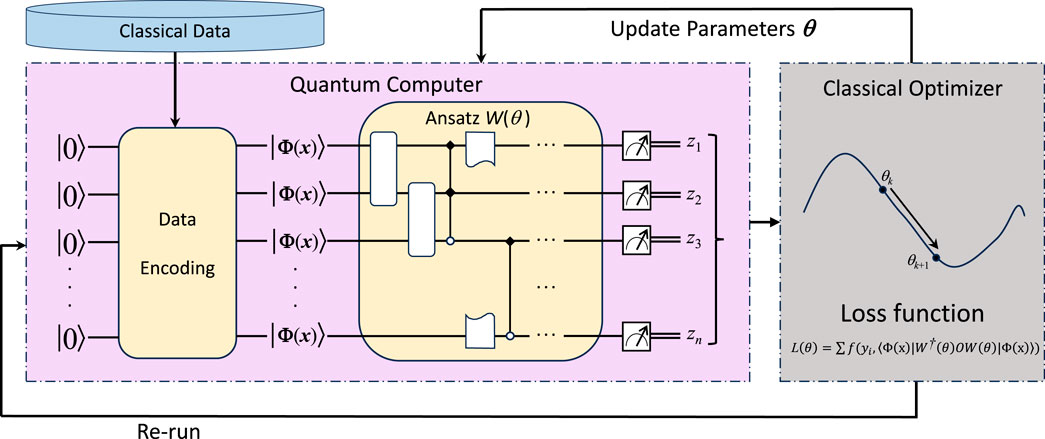
FIGURE 1. The general scheme of VQCs.

Similar to conventional supervised learning, VQCs also contain two phases: the training phase and the classifying phase. First, in the training phase, a loss function evaluates the gap between true labels and predicted values, so a classical optimizer can be employed to tune the ansatz. The goal of the training phase is to find a set of parameters that maximizes the accuracy of the classification models. Second, in the classifying phase, the encoded quantum state will evolve through the well-trained ansatz W(θ) with optimized variational parameters θ. Finally, the resulting quantum state will be measured, and a customized function f: {0,1}ⁿ → {−1, 1} is utilized to map the distribution of the measurement results to the labels.

From the aforementioned workflow, we can find that there are several factors that can potentially impact the effectiveness of VQCs, including the data encoding method, the loss function, the type of optimizers, etc. Carefully selecting methods in VQCs tailored to specific problems is crucial to achieving improved classification results. In practice, furthermore, a large amount of data is presented in the form of complex numbers, e.g., phase data for power systems and Fourier transform results on image processing. How to process and analyze such data by VQC remains a challenging problem. In the following analysis, we will delve into these factors and provide the most suitable method specifically for the case of complex-valued data.

3 Methods—VQCs for complex-valued features

3.1 Data encoding for complex-valued data

Data encoding is a methodology that transforms classical data into quantum information, which can be further processed by quantum computers. Choosing proper data encoding methods can better characterize classical data, enhancing its compatibility and interpretability within the QVC framework. Schuld (2021) has proven that data encoding is equivalent to kernel methods for supervised learning, where kernel methods are employed to project original data into a high-dimensional space. Thus, in the field of QML, the original data is also mathematically mapped into a new Hilbert space through data encoding, which serves as the mathematical framework where quantum states reside and interact. In practice, a unitary quantum circuit is commonly employed to realize the data encoding process. Specifically, the basis state |0⟩^⊗n evolves through the unitary quantum circuit to become different quantum states with input features.

So far, researchers have proposed many data encoding strategies (Biamonte et al., 2017), including basis encoding, amplitude encoding, angle encoding, etc. Data encoding methods can be achieved by building unitary quantum circuits. Rotation gates and controlled gates are the main components in these quantum circuits. By taking advantage of quantum entanglement, 2ⁿ features can be encoded into quantum states with a n-qubit quantum circuit. In this paper, a unitary quantum circuit ${\mathcal{U}}_{\mathrm{\Phi }(\mathbf{x})}$, a feature map, represents the data encoding process, and the resulting states processed by this map can be expressed as $|\mathrm{\Phi }(\mathbf{x})\rangle ={\mathcal{U}}_{\mathrm{\Phi }(\mathbf{x})}|{0\rangle }^{\otimes n}$. Next, two categories of data encoding strategies will be introduced for complex-valued data used for QML.

3.1.1 Coupling encoding method for complex-valued data

The coupling encoding method refers to encoding complex-valued data as a whole entity without splitting it into individual components and representing it in a quantum state when performing data encoding. Amplitude encoding is a type of quantum state preparation in which classical data are encoded as the amplitudes of quantum superposition states, and also one of the common data encoding methods in the field of quantum computing is one of the common data encoding methods in the field of quantum computing (Harrow et al., 2009). For a classical vector $\mathbf{x}\in {\mathbb{C}}^{2^n}$ that satisfies ${\sum }_{k=1}^{2^n}|x_k{|}^2=1$, it can be represented by the amplitudes of a quantum state |Φ(x)⟩, which is defined by Eq. 1,

$|\mathrm{\Phi }\left(\mathbf{x}\right)\rangle ={\displaystyle \sum _{k=1}^{2^n}}{x}_k|k\rangle ,(1)$

where |k⟩ is the kth computational basis.

If the original vector $\mathbf{x}\in {\mathbb{C}}^N$ is not normalized, in order to encode x through amplitude encoding, the initial step is to normalize it to ensure that it satisfies ${\sum }_{k=1}^N|x_k{|}^2=1$. This step implies that quantum states represent the data in a dimension that is one less than its original dimension. To address this issue, one approach is to add an element 1 to the given feature vector and normalize the resulting vector. For instance, for any vector $\mathbf{x}={[x_1,x_2,\dots ,x_N]}^{\text{T}}\in {\mathbb{C}}^N$ to be normalized, we can increase its dimension by one and set the added component as 1. The augmented vector $\tilde{\mathbf{x}}\in {\mathbb{C}}^{N+1}$ can be expressed as Eq. 2,

$\tilde{\mathbf{x}}={\left[x_1,x_2,\dots ,x_N,1\right]}^{\text{T}},(2)$

The augmented vector after normalization is given by Eq. 3,

$\widehat{\mathbf{x}}={\left[\frac{x_1}{\Vert \tilde{\mathbf{x}}\Vert },\frac{x_2}{\Vert \tilde{\mathbf{x}}\Vert },\dots ,\frac{x_N}{\Vert \tilde{\mathbf{x}}\Vert },\frac{1}{\Vert \tilde{\mathbf{x}}\Vert }\right]}^{\text{T}},(3)$

where $\Vert \tilde{\mathbf{x}}\Vert$ is the norm of the augmented vector $\tilde{\mathbf{x}}$. When the Euclidean norm is employed for normalization, $\Vert \tilde{\mathbf{x}}{\Vert }_2=\sqrt{{x_1}^2+{x_2}^2+\cdots +{x_N}^2+1}$. We can find that the information on the norm of the vector remains in $\widehat{\mathbf{x}}$. Therefore, by changing the N-dimensional vector to a N + 1-dimensional vector, the original data will not lose information. In the quantum phase, if an N + 1-dimensional vector is encoded into an n-qubit quantum state, the number of the quantum state n is required to satisfy n ≥ log (N + 1). Generally, n = log (N + 1) holds with a very tiny probability, so the dimension of the encoded vector is usually less than log (N + 1). When the dimension of the processed data in (3) is less than 2ⁿ, we can always extend it into a new vector with a dimension of precisely 2ⁿ by adding zero entries. Thus, the data can fit into an n-qubit quantum state.

Power systems are a vast and intricate network that encompasses extensive energy interactions and data transmission. Phasor measurement units (PMU) are a fundamental monitoring component in modern alternating current power systems Guarnieri (2013). With the large-scale deployment of PMUs, modern power systems have become easier to monitor and control. In practice, PMUs quickly capture the samples from a sinusoidal waveform (including voltage, current, and power) and compute the magnitude and phase angle of an electrical phasor quantity.

For an operating power system, the complex power S in phasor form can be expressed as Eq. 4,

$S=|S|\angle \varphi =|S|e^{j\varphi }=|S|\cos \varphi +j|S|\sin \varphi =P+jQ,(4)$

where j represents the imaginary unit, |S| and ϕ are the magnitude and the phase angle of the complex power, P denotes the active power and Q denotes the reactive power. Similarly, this property exists in various electrical quantities. Note that $S\in \mathbb{C}$ in which the amplitudes of quantum states live. Hence, the raw complex data provided by PMUs can be directly embedded in quantum states by amplitude encoding. We can also use the Bloch sphere to visualize a normalized complex electrical quantity shown as Figure 2. For high-dimensional complex power data, each feature can be embedded into the amplitude in (1) as long as the data encoding circuit with a sufficient number of qubits is available.

FIGURE 2

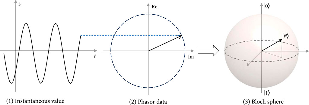
FIGURE 2. Data encoding for the phasor data in power systems.

For a power system dataset with m complex-valued features, e.g., complex power, it can be represented by a m-dimensional vector Eq. 5,

$\mathbf{s}={\left[P_1+j{Q}_1,P_2+j{Q}_2,\dots ,P_m+j{Q}_m\right]}^{\mathsf{T}}(5)$

The quantum state after amplitude encoding is represented by Eq. 6,

$|\mathrm{\Phi }\left(\mathbf{s}\right)\rangle =\left({\widehat{P}}_1+j{\widehat{Q}}_1\right)|1\rangle +\left({\widehat{P}}_2+j{\widehat{Q}}_2\right)|2\rangle +,\dots ,+\left({\widehat{P}}_m+j{\widehat{Q}}_m\right)|m\rangle +\frac{1}{\sqrt{\Vert \mathbf{s}{\Vert }_2^2+1}}|m+1\rangle ,(6)$

where ‖s‖₂ is the Euclidean norm of the vector s, and ${\widehat{P}}_i=P_i/\sqrt{\Vert \mathbf{s}{\Vert }_2^2+1}$, ${\widehat{Q}}_i=Q_i/\sqrt{\Vert \mathbf{s}{\Vert }_2^2+1}$.

An inherent advantage of amplitude encoding is that it allows for the exploitation of quantum superposition and entanglement properties, so a large number of features can be input into the QML algorithm with a limited number of qubits. Specifically, the complex vector x with 2ⁿ features can be encoded into a n-qubit quantum state by leveraging the superposition state of quantum systems. This means, by adopting amplitude encoding, data can potentially be processed in parallel, indicating a potential to reduce computational time and improve efficiency compared to classical machine learning methods.

3.1.2 Splitting encoding methods for complex-valued data

Contrary to the coupling encoding method, the splitting encoding method involves processing the real part and the imaginary part of complex-valued data separately. Many data encoding methods only accept real numbers as the parameters of their quantum circuits, e.g., angle encoding and Pauli feature map. For this type of data encoding method, we have to separate the real parts and the imaginary parts, so we can further embed them into quantum states.

3.1.2.1 Angle encoding

Angle encoding is a common data encoding method based on rotation gates. It utilizes the angles of quantum gates as parameters to encode classical information in quantum states and can be applied to different forms of data (Schuld, 2021), such as binary, real-valued, or categorical data. Therefore, angle encoding does not necessitate classical data normalization, meaning that data preprocessing for angle encoding is not required. The basic angle encoding with a single layer of Pauli rotation gates is given by Eq. 7,

$|\mathrm{\Phi }\left(\mathbf{x}\right)\rangle ={\otimes }_{i=1}^n\left(R_i\left(x_i\right)|0\rangle \right),(7)$

where R_i represents the rotation gate of ith qubit, which can be expressed as the exponential form of Pauli matrices σ, where σ ∈ {I, X, Y, Z}.

Furthermore, a more intricate quantum circuit with multiple layers and repetitions for complex-valued angle encoding can be constructed by incorporating more layers of Pauli rotation gates, i.e., Figure 3, where H is the Hadamard gate that maps |0⟩ to $\frac{1}{\sqrt{2}}|0\rangle +\frac{1}{\sqrt{2}}|1\rangle$. Nonetheless, for angle encoding, the number of qubits is equal to the dimension of features as only rotation gates exist in the data encoding circuits, which limits the potential exploitation of quantum entanglement benefits.

FIGURE 3

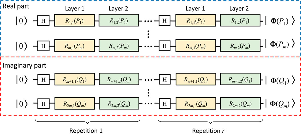
FIGURE 3. An angle encoding architecture for complex-valued data with multiple repetitions. R_i,j represents the rotation gate of ith qubit in jth layer, different colored blocks indicate the utilization of different rotation gates within the data encoding architecture. The yellow and green boxes correspond to R_y and R_z rotation gates, respectively.

For the dataset being the same as Eq. 5, the quantum state after processing by the angle encoding in Figure 3 can be represented as Eq. 8,

$|\mathrm{\Phi }\left(\mathbf{s}\right)\rangle =\prod _{k=1}^c\left[\left[{\otimes }_{i=1}^m{R}_{i,1}\left(P_i\right)R_{i,2}\left(P_i\right)\right]\otimes \left[{\otimes }_{i=1}^m{R}_{m+i,1}\left(Q_i\right)R_{m+i,2}\left(Q_i\right)\right]\otimes H^{\otimes 2m}\right]|{0\rangle }^{\otimes 2m},(8)$

where c is the number of repetitions in 3.

3.1.2.2 Pauli feature map

Pauli feature map was first proposed in Havlíček et al. (2019), and it represents a family of data encoding methods. It can be formulated as follows Eqs 9, 10,

${\mathcal{U}}_{\mathrm{\Phi }\left(\mathbf{x}\right)}=U_{\mathrm{\Phi }\left(\mathbf{x}\right)}{H}^{\otimes n}\dots U_{\mathrm{\Phi }\left(\mathbf{x}\right)}{H}^{\otimes n},(9)$

$U_{\mathrm{\Phi }\left(\mathbf{x}\right)}=e^{\left(j{\displaystyle \sum _{C\subseteq \left[n\right]}}{\varphi }_C\left(\mathbf{x}\right)\prod _{i\in C}{\sigma }_i\right)},(10)$

where [n] means the enumeration of n qubits, and C describes the interconnections between individual qubits. Theoretically, C is very large when the number of qubits is high, which renders the implementation of the Pauli feature map more intricate. Therefore, we have |C| ≤ 2 in this paper, so the Pauli feature map can be efficiently implemented. ϕ_C(x) is a set of linear f_l(x) and the non-linear f_nl(x) functions of the original data. Havlíček et al. (2019) provides examples of functions utilized for the Pauli feature map, which are defined as follows Eqs 11, 12,

${\varphi }_k\left(x\right)=x_k,(11)$

${\varphi }_{m,n}\left(x\right)=\left(\pi -x_m\right)\left(\pi -x_n\right),(12)$

where ϕ_k(x) is the encoding functions embedded in single-qubit-gate unitary, and ϕ_m,n(x) is the encoding functions embedded in two-qubit-gate unitary. The repetition of H and U_Φ(x) can be adjusted to pursue better performance for VQCs. For instance, given the trade-off between the circuit depth and its performance, the provided feature map in Havlíček et al. (2019) consists of two Hadamard transforms and uses the Ising model, and it has shown good performance for their classification tasks. When specifying to power system applications, the Pauli feature map is given in Figure 4.

FIGURE 4

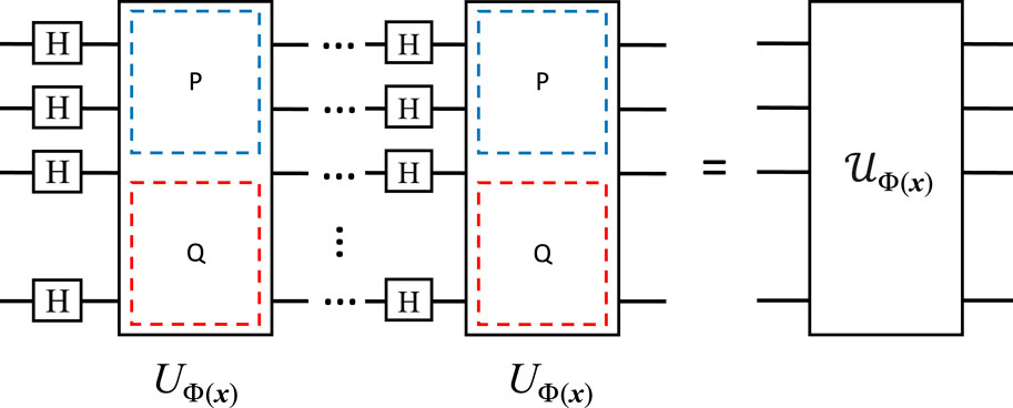
FIGURE 4. Pauli feature map for complex-valued data.

For the dataset being the same as (5), the quantum state after processing by the Pauli feature map with two repetitions can be represented as Eq. 13,

$|\mathrm{\Phi }\left(\mathbf{s}\right)\rangle =U_{\mathrm{\Phi }\left({\mathbf{s}}_f\right)}{H}^{\otimes m}{U}_{\mathrm{\Phi }\left({\mathbf{s}}_f\right)}{H}^{\otimes m}|{0\rangle }^{\otimes m},(13)$

where ${\mathbf{s}}_f={[P_1,Q_1,P_2,Q_2,\dots ,P_m,Q_m]}^{\mathsf{T}}\in {\mathbb{R}}^{2m}$.

Pauli feature maps, compared with angle encoding, exhibit the ability to handle diverse data types, but offer the potential for quantum advantage through the exploitation of quantum parallelism and entanglement. Nevertheless, the considerable number of quantum gates and qubits required can pose challenges. Moreover, its complex structure and the extensive number of gates can result in a deep circuit, leading to the encoding circuit being more susceptible to noise and errors in current quantum hardware.

3.2 Parameterized quantum circuits of VQCs for complex-valued data

Parameterized quantum circuits are typically referred to as ansatz in the quantum computing field. They are a critical part of VQCs, whose structure plays a crucial role in determining the final parameters, thereby influencing the training process to achieve optimal results. Among the various ansatzes, layered hardware-efficient ansatzes have been prominently used for general-purpose problems. What is even more noteworthy is that quantum circuits can be constructed with fewer layers or parameters thanks to the symmetry and locality properties inherent in quantum circuits (Iblisdir et al., 2014). Generally, ansatz architecture usually employs a kind of universal and ‘problem-agnostic’ parameterized quantum circuits, so they can be utilized as the training quantum circuit even in those situations where no relevant information is readily accessible.

For a general parameterized quantum circuit, the training parameters are embedded in unitary operators W(θ) consisting of a collection of basic quantum gates, including some parameterized and unparameterized gates. By increasing the depth of a parameterized quantum circuit, the number of variational parameters θ also increase, through which the function-fitting capabilities of ansatz are expected to be improved. For W(θ), it can be represented by the product of a series of unitaries Eq. 14,

$W\left(\mathit{\theta }\right)=W_l\left({\mathit{\theta }}_l\right)\dots W_2\left({\mathit{\theta }}_2\right)W_1\left({\mathit{\theta }}_1\right)(14)$

where l is the number of layers in ansatz.

In this paper, an ansatz initially proposed in Kandala et al. (2017) is implemented for the classification issue of complex-valued data, as shown in Figure 5, which contains single-qubit rotation gates with variational parameters and entangling unitaries with fixed phases. Each single-qubit-gate unitary is followed by an entangling unitary, except for the final unitary W_l (θ_l). This ansatz architecture leads to better performance on superconducting quantum processors, as summarized in Kandala et al. (2017).

FIGURE 5

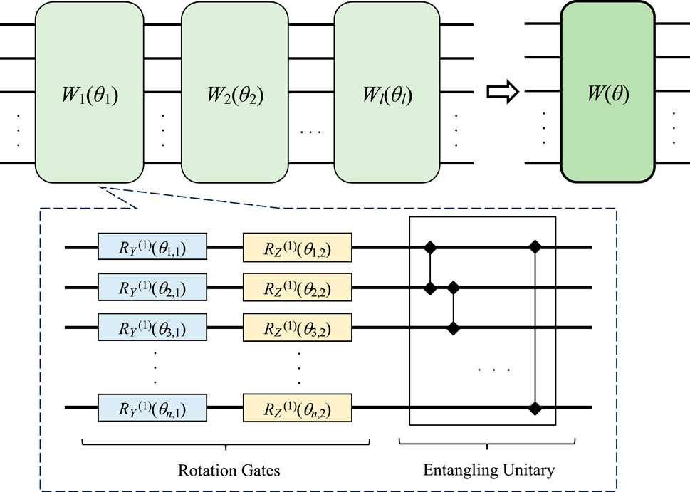
FIGURE 5. The demonstration of layered parameterized quantum circuit.

In Figure 5, the variational parameters only exist in the rotation gates. Experimental validation in Kandala et al. (2017) has demonstrated that entangling unitaries with fixed phases exhibit superior performance compared to entangling unitaries with variational parameters. Thus, the number of variational parameters in the ansatz comes to 3ln, where n is the number of implementing qubits.

In order to reduce the complexity of the VQC, we only use Pauli Y and Pauli Z rotations in the single-qubit-gate unitaries defined by (15), which represents a set of rotation gates in a layer of W(θ) in Figure 5,

$U_{\text{loc\hspace{0.17em}}}^{\left(l\right)}\left({\mathit{\theta }}_l\right)={\otimes }_{m=1}^{n}U\left({\mathit{\theta }}_{m,t}\right),(15)$

where ${\mathit{\theta }}_l\in {\mathbb{R}}^{2n}$, and ${\mathit{\theta }}_{m,t}\in {\mathbb{R}}^2$, and $U\left(\mathit{\theta }\right)$ is defined as Eq. 16,

$U\left({\mathit{\theta }}_{m,t}\right)=e^{j\frac{1}{2}{\theta }^z{Z}_m}{e}^{j\frac{1}{2}{\theta }^y{Y}_m},(16)$

where Y_m means the mth Pauli Y matrix and Z_m means the mth Pauli Z matrix.

To further simplify the construction of the ansatz, we can build the entangling unitary based on the Ising model. The controlled-Z gates are utilized as entanglement gates, which only entangle with the neighboring qubits. The entanglement unitary is given by (17), which represents the entangling unitary in a layer of W(θ) in Figure 5.

$U_{\text{ent}}=\prod _{\left(i,j\right)\in E}\mathrm{C}\mathrm{Z}\left(i,j\right),(17)$

where E represents the collection of neighboring qubits, and CZ (i, j) represents the controlled Z gates applied at qubit i and j.

In this setting Eq. 14 can be expanded in a more detailed manner Eq. 18, and the structure of the VQC used is shown in Figure 5,

$W\left(\mathit{\theta }\right)=U_{\text{loc}}^{\left(l\right)}\left({\mathit{\theta }}_l\right)U_{\text{ent}}\dots U_{\text{loc}}^{\left(2\right)}\left({\mathit{\theta }}_2\right)U_{\text{ent}}{U}_{\text{loc}}^{\left(1\right)}\left({\mathit{\theta }}_1\right),(18)$

where $U_{\text{loc}}^{(l)}\left({\mathit{\theta }}_l\right)$ denotes the lth single-qubit-gate unitary, and U_ent represents the entangling unitary.

As the number of input qubits increases, the depth of the proposed VQCs needs to be incrementally increased to meet the demand for better expressivity. However, considering the rapid increase in the number of parameters arising from deeper quantum circuits, the number of layers in the ansatz is set to 2 in this paper, as detailed in Section 4.

3.3 Loss functions and optimizers of VQCs for complex-valued data

3.3.1 Loss functions

For a complex-valued dataset with labels, such as power system data with stable and unstable scenarios, the loss function is designed in VQCs to learn the relationship between the power system data and the stability characteristics, i.e., the label of each operational scenario. Thus, we can assess power system stability from test data. Thus, the choice of the loss function has a significant effect on the optimization process, as it alters the landscape of the optimization problem. Therefore, the loss function needs to be carefully selected. For classification tasks, in general, the loss function can be defined as the error between the true label and the expectation value under an observable O. Basically, the observable O here serves as a bridge between the final quantum states and the data label {+1, −1}. Mathematically, the observable can be viewed as an operator and has eigenvalues either +1 or −1, so the expectation value ⟨Φ(x_i)|W^†(θ)OW(θ)|Φ(x_i)⟩ under the observable O can be bounded by [−1, +1]. It can be further utilized to assess the gap to labels by tuning the parameters in the ansatz. In quantum physics, the observable O measures the property of quantum states by means of successive operations, e.g., applying electromagnetic fields, and eventually reading a value in [−1, +1]. The general form of the loss function can be given by Eq. 19,

$L\left(\mathit{\theta }\right)={\displaystyle \sum _i}f\left(y_i,⟨\mathrm{\Phi }\left({\mathbf{x}}_{\mathbf{i}}\right)|W^{†}\left(\mathit{\theta }\right)OW\left(\mathit{\theta }\right)|\mathrm{\Phi }\left({\mathbf{x}}_{\mathbf{i}}\right)⟩\right),(19)$

where f denotes the loss function, and y_i is the label of ith sample.

In the field of traditional machine learning, various loss functions with favorable capabilities have been proposed (Alpaydin, 2010). Correspondingly, these loss functions can also be utilized in VQCs to tackle classification problems effectively. Here we provide examples for designing the loss function.

(1) l1 and l2 loss functions: The squared loss, also called l2 loss, is frequently selected as the preferred loss function, and Eq. 19 can be reformulated as Eq. 20,

$L_{l2}\left(\mathit{\theta }\right)={\displaystyle \sum _i}{\left(y_i-⟨\mathrm{\Phi }\left({\mathbf{x}}_{\mathbf{i}}\right)|W^{†}\left(\mathit{\theta }\right)OW\left(\mathit{\theta }\right)|\mathrm{\Phi }\left({\mathbf{x}}_{\mathbf{i}}\right)⟩\right)}^2(20)$

Another typical loss function replaces (⋅)² with absolute value |⋅|, which is named l1 loss.

(2) Cross-entropy loss function: The cross-entropy loss based on information theory is also popular in QML. It also exhibits the property of convexity, akin to the square function, making it well-suited for gradient descent optimization methods (Murphy, 2012). The expression is defined as Eq. 21,

$L_{\mathit{ent}}\left(\mathit{\theta }\right)={\displaystyle \sum _i}-y_i\text{log}{p}_i-\left(1-y_i\right)\text{log}\left(1-p_i\right),(21)$

where p_i = ⟨Φ(x_i)|W^†(θ)OW(θ)|Φ(x_i)⟩ in VQCs.

(3) Misclassification-based loss function: This loss function is formulated to assess the performance of VQCs by evaluating the probability of occurrence of misclassified samples. Havlíček et al. (2019) introduces a loss function for binary classification, which shows a good result in their classification tasks. Here we provide a brief overview of it. By evaluating the ratio of misclassified samples, the loss function can be defined as Eq. 22,

$P_{\text{err}}=\frac{1}{|T|}\left({\displaystyle \sum _y}{\displaystyle \sum _{s\in T_y}}\mathrm{P}\mathrm{r}\left({\tilde{m}}_T\left(s\right)\ne y\mid s\in T_y\right)\right),(22)$

where |T| is the total number of samples. T_y is the sample subset labeled by y. ${\tilde{m}}_T(s)$ is the measurement result for the samples of the subset T_y.

The estimation of misclassifying ratio can be thought of as carrying out experiments R times for each sample, which follow a binomial distribution. Thus, the probability of misclassification is given by Eq. 23,

$\mathrm{P}\mathrm{r}\left({\tilde{m}}_T\left(s\right)\ne y\mid s\in T_y\right)={\displaystyle \sum _{i=0}^{\frac{R}{2}}}\left(\begin{array}{c}\hfill R\hfill \\ \hfill i\hfill \end{array}\right)p_y^i{\left(1-p_y\right)}^{R-i},(23)$

where R/2 means that a sample is misclassified when less than half of the measurements in R experiments are not the state corresponding to the true label. The probability of classification labels y is expressed as Eq. 24,

$p_y=\frac{1}{2}\left(1+y⟨\mathrm{\Phi }\left(\mathbf{x}\right)\left|W^{†}\left(\mathit{\theta }\right)OW\left(\mathit{\theta }\right)\right|\mathrm{\Phi }\left(\mathbf{x}\right)⟩\right),(24)$

In practice, p_y can be estimated by $p_y=\frac{r_y}{R}$, where r_y is the number of occurrences of samples labeled by y.

When R is very large, the probability of misclassification can be further expressed as Eq. 25. See (Havlíček et al., 2019) for details.

$\mathrm{P}\mathrm{r}\left({\tilde{m}}_T\left(s\right)\ne y\mid s\in T_y\right)\approx \mathrm{s}\mathrm{i}\mathrm{g}\left(\sqrt{R}\frac{\frac{1}{2}-p_y}{\sqrt{2\left(1-p_y\right)p_y}}\right)(25)$

3.3.2 Optimzers for VQCs

In order to obtain the optimal parameters of ansatz, an optimizer implemented in classical computers makes queries to the quantum device repeatedly and searches for a set of parameters better than the current one. Optimizers can be divided into two categories based on whether or not analytical gradients are required, as gradients are usually used to speed up finding the minimum value of loss functions.

(1) The first category of optimizers is the gradient-free optimizers, e.g., the Simplex algorithm and simultaneous perturbation stochastic approximation (SPSA). The Simplex algorithm is an optimizer designed to find the minimum value when the derivative of the objective function is unknown, making it a gradient-free and easy-to-implement method. Constrained optimization by linear approximations (COBYLA) is one of the most widely used approaches based on the Simplex method, especially in the optimization of ansatz (Powell, 2007). The COBYLA is a sequential trust-region optimization technique that relies on linear approximations. These approximations are constructed using linear interpolation at n + 1 points in the variable space, ensuring the maintenance of a well-formed simplex throughout the iterations. It is particularly suitable for solving non-smooth and nonlinear optimization problems with a moderate number of variables.

There is an alternative optimization approach that does not rely on accessing the gradient. If the derivative of the cost function is difficult to access, numerical methods can be used to approximate the gradient. A typical example of such an algorithm is SPSA introduced in Spall (2005). Although it does not require the analytical expression of gradients, it approximates the gradient by perturbing the parameters of the optimization problem in a stochastic way, thereby adjusting the direction of optimization. By utilizing random and simultaneous perturbation, SPSA can process noisy and non-differentiable objective functions with a relatively fast convergence speed.

(2) Another category of optimizers is the gradient-based optimizers. Gradient-based optimizers require the calculation of analytical derivatives to tune the ansatz in VQCs. The most common algorithm is the gradient descent, which is given by Eq. 26,

${\widehat{\mathit{\theta }}}^{k+1}={\widehat{\mathit{\theta }}}^k-{\alpha }^k\nabla L\left({\widehat{\mathit{\theta }}}^k\right),(26)$

where ${\widehat{\mathit{\theta }}}^k$ means the current parameters, α^k is the learning rate and $\nabla L({\widehat{\mathit{\theta }}}^k)$ is the estimated gradient at kth iteration.

Computing the analytical gradients of a loss function always involves the derivatives of quantum circuit operators. The phase shift strategy can be further utilized to compute derivatives with little computing resources (Schuld et al., 2019). Among the popular gradient-based optimizers in the quantum domain, well-known ones include Conjugate Gradient Optimizer (CG) and Analytic Quantum Gradient Descent (AQGD), etc.

We compared the performance of different optimization algorithms in the data set of the power system in the following numerical examples.

4 Results

In this section, we obtain complex-valued data from a microgrid system to validate the effectiveness of the VQC developed in this paper, as shown in Figure 6. All power system simulations are conducted using the Power System Analysis Toolbox (PSAT) in the MATLAB environment. The microgrid system contains 10 buses, 5 renewable energy sources, and 5 power loads. Since changing generator power and load power may lead to power system instability, this system can operate at various equilibrium points by setting different active and reactive power demands of loads and generations of renewable energy sources. Time-domain simulations were employed to identify the stability of the power system operating at different equilibrium points (Milano, 2005). A total of 366 stable samples and 602 unstable samples were created for the experiment. Each equilibrium point contains various features (e.g., bus voltage, frequency, active power flow, reactive power flow, etc.) under both stable and unstable scenarios. In this paper, only active power and reactive power (a total of 10 real-valued features) in the renewable energy sources buses are selected as the key features to input into the VQC, which can be combined to form complex power as the input of complex-valued amplitude encoding. The label of unstable samples is set to −1 and the label of stable samples is set to 1. The generated dataset is divided into the training set and the test set, and the training set data accounts for 80% of the total dataset. We selected 10 stable samples and 10 unstable samples to visualize their features, shown in Figure 7. For each sample, active power and reactive power in 5 power source buses (total 10 features) are selected for data visualization. The unstable samples will lead to power oscillations with increasing amplitude, which could make the power system crash eventually. The stable samples will cause power oscillations with decreasing amplitude, and the oscillations will disappear finally and the power system will be running at a new equilibrium point normally.

FIGURE 6

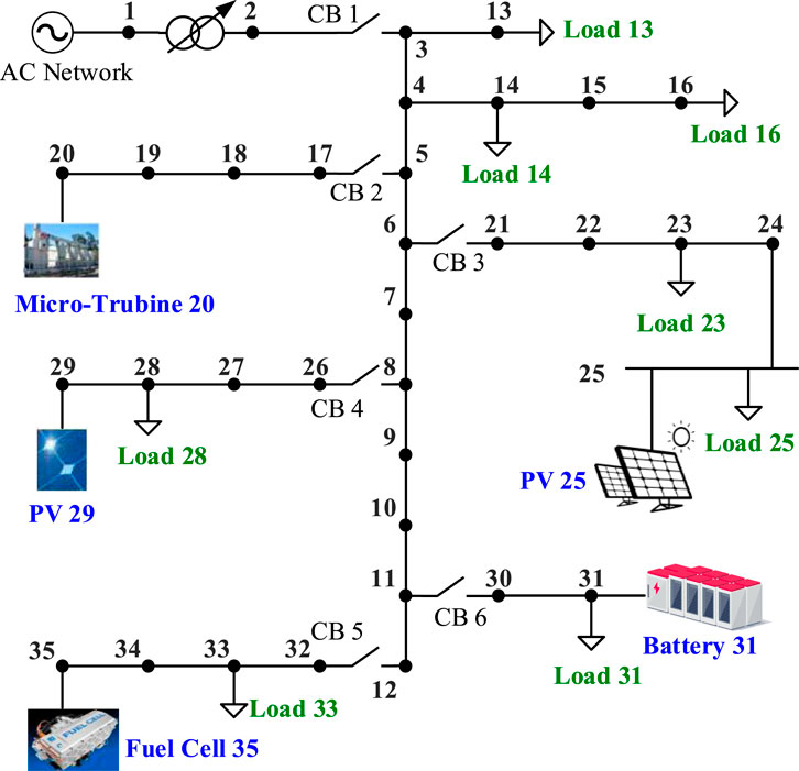
FIGURE 6. A microgrid system containing renewable energy sources and power loads.

FIGURE 7

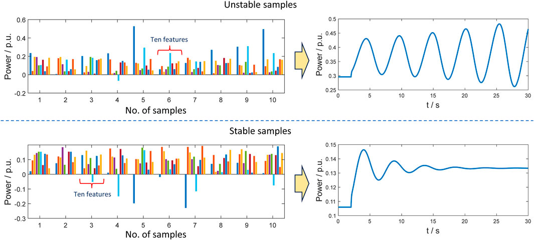
FIGURE 7. Data visualization for active power and reactive power of stable and unstable scenarios. The label of the x-axis indicates 10 different sets of samples, each containing 10 features. For each sample, it induces dynamic behavior in the system, leading to either convergence or divergence, similar to the trajectories shown in the right panel.

In our experimental study, all related quantum circuits associated with the data encoding methods and the VQCs are formulated using the Qiskit simulator. A random initialized VQC built in Section 3.2 is employed to execute the classification task. The objective of the VQC is to directly distinguish the unstable samples of equilibrium points from those stable ones based on the features generated. This section investigates the impact of data encoding methods, loss functions, and optimizers on the final classification results of VQCs when applied to the power system dataset.

4.1 Comparison of data encoding methods

Different data encoding methods could have different abilities to characterize the features in datasets. In this section, the coupling data encoding strategy and the splitting data encoding strategy were explored on the microgrid dataset. The active power and the reactive power generation of renewable energy sources were used as the input of VQC. In order to reflect which data encoding method is more suitable for power system data, here we adopted the squared error as the loss function and the COBYLA as the optimizer for each training. Besides, we used the same two layers in the parameterized quantum circuit to compare the experimental results of different data encoding methods.

Five types of data encoding methods were applied to encode the power system features, including two angle encoding methods, Pauli feature map, splitting amplitude encoding, and coupling amplitude encoding. The designs of the angle encoding circuits adopted are shown in Figure 8, and the Pauli feature maps are constructed as the structure in Section 3.1.2. They all consist of the Hadamard gates and the Pauli rotation gates, and they have two same repetitions to strike a balance between performance and circuit depth. In addition, in order to achieve better performance on angle encoding methods and the Pauli feature map, we used a data dimensionality reduction method to reduce the dimension of the features before performing the classification of VQCs. Hence, in this section, we utilized both the original data and the data processed by principal component analysis (PCA) as the input features of VQCs to obtain comprehensive experimental results. The principal components corresponding to the largest three eigenvalues were selected as the input features. Considering the active power and the reactive power can be represented as a vector on the complex plane, the proposed complex-valued amplitude encoding is used for encoding the complex power. The number of quantum gates used for different data encoding methods is shown in Table 1.

FIGURE 8

FIGURE 8. The designs of angle encoding: (A) Angle encoding A, (B) Angle encoding B.

TABLE 1

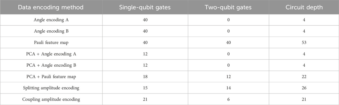
TABLE 1. The number of quantum gates used for different data encoding methods.

In this section, to better evaluate the classification model, we use four types of indexes, including accuracy, precision, recall, and F1-score, which are widely used in binary classification. They are defined as Eqs 27–30,

$Accuracy=\frac{TP+TN}{TP+TN+FP+FN},(27)$

$Precision=\frac{TP}{TP+FP},(28)$

$Recall=\frac{TP}{TP+FN},(29)$

$F1-Score=\frac{2*Precision*Recall}{Precision+Recall},(30)$

where TP denotes the number of true positives, TN the number of true negatives, FP the number of false negatives, and FN the number of false negatives. The results of VQCs on the test dataset for different data encoding methods are shown in Table 2. The data distribution processed by PCA is shown in Figure 9.

TABLE 2

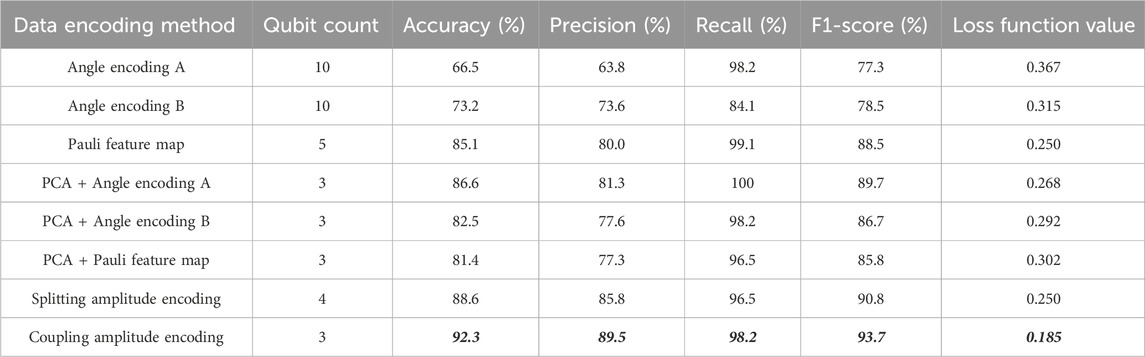
TABLE 2. Numerical result for different data encoding methods.

FIGURE 9

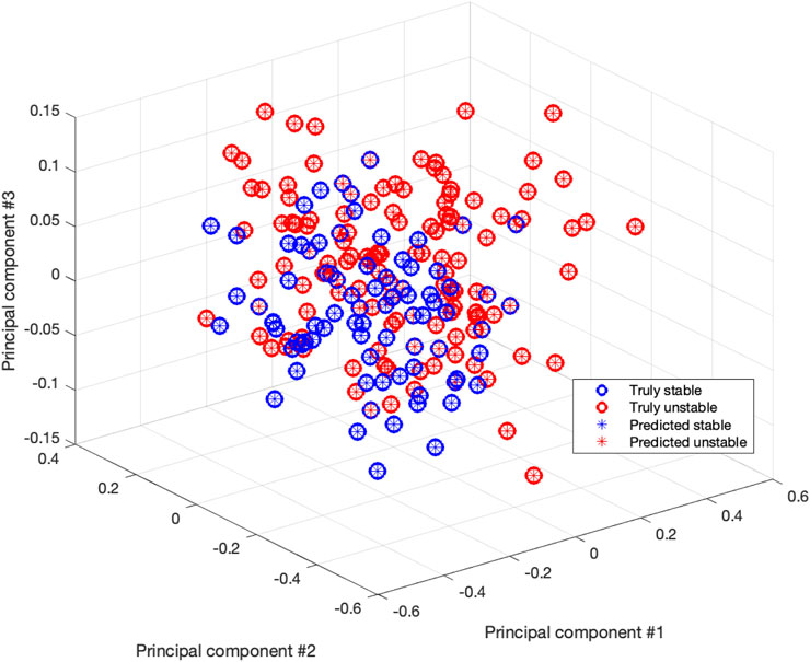
FIGURE 9. Stable and unstable samples distribution processed by PCA.

From Table 2, we can see that,

• The coupling amplitude encoding can achieve 92.3% accuracy on the microgrid dataset, which performs better than the other data encoding methods. Angle encoding A, Angle encoding B, the Pauli feature map and the splitting amplitude encoding can not achieve over 90% accuracy on the test data.

• Angle encoding A and Angle encoding B yield notably unfavorable outcomes, a consequence attributed to the increase of qubits count in VQCs, thereby rendering optimization challenging.

• After applying PCA to the data, the performance of the method has been improved overall, due to the shallow depth of the parameterized quantum circuit. The barren plateau issue would become more intractable with increasing size of qubit count. We find that there is also a decrease in the accuracy of the VQC model when the qubit count has to be increased due to different coding methods used in the numerical results.

4.2 Comparison of loss functions

The choice of loss function directly influences the optimization landscape of VQCs. Choosing appropriate loss functions can aid in the development of a more effective and efficient classification model. In this section, four types of loss functions are investigated, including l1 loss, l2 loss, cross-entropy loss, and the misclassification-based loss function proposed in Havlíček et al. (2019). To showcase which loss function performs better for this problem, we use the dimensional-reduced microgrid system data processed by PCA, and fix the data encoding method as the coupling amplitude encoding and employed the COBYLA as the optimizer. The numerical results for the four loss functions are shown in Table 3, and optimization landscapes are shown in Figure 10.

TABLE 3

TABLE 3. Numerical result for different loss functions on testing dataset.

FIGURE 10

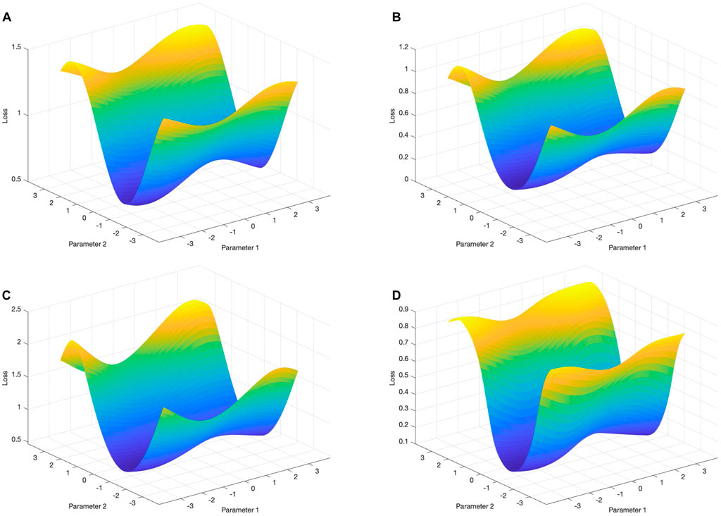
FIGURE 10. Optimization landscapes of the second two parameters θ_2,1 and θ_2,2 in Figure 5 when other parameters are optimal: (A) l1 loss function, (B) l2 loss function, (C) cross-entropy loss function, (D) misclassification-based loss function.

From Table 3, we can find that,

• The l1 loss function exhibits poor optimization performance for the proposed VQC. Figure 10A shows the minimum of the landscape is close to 0.5. Compared to l2 loss function in Figure 10B, the l1 loss function yields a significantly higher minimum value.

• Among the tested loss functions, the performance of the l2 loss function and the misclassification-based loss function excels in the classification tasks, both achieving the highest accuracy 92.3%. The l1 loss function and the cross-entropy loss function yield comparatively low accuracy.

• These loss functions may exhibit barren plateaus. If gradient-based optimizers are utilized to find the minimum of the loss function, barren plateaus may be a daunting challenge for optimization. Furthermore, they all exhibit landscapes with multiple local optimums that could hinder the optimizer from finding the global optimum.

4.3 Comparison of optimizers

Optimizers play a pivotal role in optimization problems. In this section, we examined four common types of optimizers used for VQC optimization, aiming to investigate the performance of various optimization methods. The tested optimizers not only include the gradient-free methods, i.e., COBYLA and SPSA, but also gradient-based methods, i.e., AQGD and CG. We also utilize the data processed by PCA as the input features. Since we found that the difference in results between different optimizers was small when using the coupling amplitude encoding, the two kinds of angle encoding methods and the Pauli feature maps are employed as the data encoding methods in the test. The l2 loss function is utilized as the loss function. Figure 11 shows the training process of different optimizers by using the Angle encoding A. Uniform distribution was employed to realize the random initialization of the VQC training. More specifically, random numbers from −π to π are drawn uniformly as the initial parameters of the VQC. The maximum number of iterations is set to 2000, 500, 100 and 70, corresponding to COBYLA, SPSA, CG and AQGD respectively. The gradient norm tolerance of CG is set to 10^–5 and the learning rate of AQGD is set to 1.0. Table 4 shows the accuracy of the proposed VQC under different optimizers and encoding methods.

FIGURE 11

FIGURE 11. Training process of different optimizers: (A) COBYLA, (B) SPSA, (C) CG, (D) AQGD.

TABLE 4

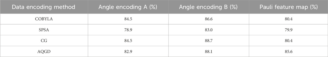
TABLE 4. Numerical result for different optimizers.

From Figure 11 and Table 4, we can find that,

• The tested optimizers have comparable capabilities to find the optimal parameters of the VQC. The gradient-based methods slightly outperform the gradient-free methods in terms of classification accuracy. Specifically, the gradient-based method AQGD and CG show better performance than gradient-free methods for searching the optimal parameters of VQCs. Furthermore, the training process of SPSA fluctuates, leading to a slight accuracy decrease compared other three optimizers.

• The COBYLA took less time to find the optimum because the parameter count is limited in this experiment. With the growth of the number of qubits and variational parameters, the gradient-based methods are expected to exhibit higher efficiency.

5 Conclusion

This study introduces a new type of VQC designed specifically for data in the complex domain. Research focuses on a comparative analysis of various factors that have the potential to impact VQC performance. Leveraging the inherent information of quantum states, the coupling amplitude encoding approach exhibits a greater ability to capture the intrinsic nature of complex numbers, surpassing the efficacy of traditional splitting data encoding methods. To operationalize these insights, the research proceeds to implement the VQC framework, employing the coupling data encoding method to achieve a highly accurate classification of labeled complex-valued data. To further elevate the performance of VQCs, this study evaluates and compares several techniques, including data encoding, loss function, and optimizer, all tailored to the demands of power system tasks. This in-depth assessment not only offers valuable insights but also serves as a guide for selecting optimal methods to effectively train the model. The comprehensive evaluations conducted in this study consistently underscore the advance of coupling amplitude encoding in complex-valued data classification within the VQC framework. The results highlight its superiority over alternative data encoding methods, reinforcing its potential to significantly enhance VQC performance.

Data availability statement

The raw data supporting the conclusions of this article will be made available by the authors, without undue reservation.

Author contributions

JC: Writing–original draft. YL: Writing–review and editing.

Funding

The author(s) declare that no financial support was received for the research, authorship, and/or publication of this article.

Acknowledgments

This work is supported by the Office of Naval Research under the award N00014-22-1-2504. The authors thank Dr. Phil Lotshaw at Oak Ridge National Laboratory and Dr. Hong Chen at PJM Interconnection for their important feedback on the manuscript.

Conflict of interest

The authors declare that the research was conducted in the absence of any commercial or financial relationships that could be construed as a potential conflict of interest.

Publisher’s note

All claims expressed in this article are solely those of the authors and do not necessarily represent those of their affiliated organizations, or those of the publisher, the editors and the reviewers. Any product that may be evaluated in this article, or claim that may be made by its manufacturer, is not guaranteed or endorsed by the publisher.

References

Alpaydin, E. (2010). Introduction to machine learning. Adaptive computation and machine learning. 2nd ed. Cambridge, Mass: MIT Press. OCLC: ocn317698631.

Google Scholar

Arute, F., Arya, K., Babbush, R., Bacon, D., Bardin, J. C., Barends, R., et al. (2019). Quantum supremacy using a programmable superconducting processor. Nature 574, 505–510. doi:10.1038/s41586-019-1666-5

PubMed Abstract | CrossRef Full Text | Google Scholar

Biamonte, J., Wittek, P., Pancotti, N., Rebentrost, P., Wiebe, N., and Lloyd, S. (2017). Quantum machine learning. Nature 549, 195–202. doi:10.1038/nature23474

PubMed Abstract | CrossRef Full Text | Google Scholar

Cerezo de la Roca, M. V. S., Arrasmith, A. T., Babbush, R., Benjamin, S. C., Endo, S., Fujii, K., et al. (2021). Variational quantum algorithms. Nat. Rev. Phys. 3, 625–644. doi:10.1038/s42254-021-00348-9

CrossRef Full Text | Google Scholar

Cong, I., Choi, S., and Lukin, M. D. (2019). Quantum convolutional neural networks. Nat. Phys. 15, 1273–1278. doi:10.1038/s41567-019-0648-8

CrossRef Full Text | Google Scholar

Farhi, E., Goldstone, J., and Gutmann, S. (2014). A quantum approximate optimization algorithm. arXiv: Quantum Physics

Google Scholar

Farhi, E., and Neven, H. (2018). Classification with quantum neural networks on near term processors. arXiv: Quantum Physics

Google Scholar

Gambetta, J. (2021). Ibm quantum roadmap to build quantum-centric supercomputers.

Google Scholar

Grover, L. K. (1996). “A fast quantum mechanical algorithm for database search,” in Proceedings of the twenty-eighth annual ACM symposium on Theory of computing - stoc ’96 (Philadelphia, Pennsylvania, United States: ACM Press), 212–219. doi:10.1145/237814.237866

CrossRef Full Text | Google Scholar

Guarnieri, M. (2013). The alternating evolution of dc power transmission [historical]. IEEE Ind. Electron. Mag. 7, 60–63. doi:10.1109/MIE.2013.2272238

CrossRef Full Text | Google Scholar

Harrow, A. W., Hassidim, A., and Lloyd, S. (2009). Quantum algorithm for linear systems of equations. Phys. Rev. Lett. 103, 150502. doi:10.1103/PhysRevLett.103.150502

PubMed Abstract | CrossRef Full Text | Google Scholar

Havlíček, V., Córcoles, A. D., Temme, K., Harrow, A. W., Kandala, A., Chow, J. M., et al. (2019). Supervised learning with quantum-enhanced feature spaces. Nature 567, 209–212. doi:10.1038/s41586-019-0980-2

PubMed Abstract | CrossRef Full Text | Google Scholar

Hendrickx, N. W., Lawrie, W. I. L., Russ, M., Van Riggelen, F., De Snoo, S. L., Schouten, R. N., et al. (2021). A four-qubit germanium quantum processor. Nature 591, 580–585. doi:10.1038/s41586-021-03332-6

PubMed Abstract | CrossRef Full Text | Google Scholar

Iblisdir, S., Cirio, M., Boada, O., and Brennen, G. K. (2014). Low depth quantum circuits for Ising models. Ann. Phys. 340, 205–251. doi:10.1016/j.aop.2013.11.001

CrossRef Full Text | Google Scholar

Kandala, A., Mezzacapo, A., Temme, K., Takita, M., Brink, M., Chow, J. M., et al. (2017). Hardware-efficient variational quantum eigensolver for small molecules and quantum magnets. Nature 549, 242–246. doi:10.1038/nature23879

PubMed Abstract | CrossRef Full Text | Google Scholar

Milano, F. (2005). An open source power system analysis toolbox. IEEE Trans. Power Syst. 20, 1199–1206. doi:10.1109/TPWRS.2005.851911

CrossRef Full Text | Google Scholar

Mitarai, K., Negoro, M., Kitagawa, M., and Fujii, K. (2018). Quantum circuit learning. Phys. Rev. A 98, 032309. doi:10.1103/physreva.98.032309

CrossRef Full Text | Google Scholar

Murphy, K. P. (2012). Machine learning: a probabilistic perspective. Adaptive computation and machine learning series. Cambridge, MA: MIT Press.

Google Scholar

Nielsen, M. A., and Chuang, I. L. (2010). Quantum computation and quantum information: 10th anniversary edition. Cambridge, MA: Cambridge University Press. doi:10.1017/CBO9780511976667

CrossRef Full Text | Google Scholar

Powell, M. (2007). A view of algorithms for optimization without derivatives. Math. TODAY 43.

Google Scholar

Schuld, M. (2021). Supervised quantum machine learning models are kernel methods.

Google Scholar

Schuld, M., Bergholm, V., Gogolin, C., Izaac, J., and Killoran, N. (2019). Evaluating analytic gradients on quantum hardware. Phys. Rev. A 99, 032331. doi:10.1103/physreva.99.032331

CrossRef Full Text | Google Scholar

Schuld, M., and Killoran, N. (2019). Quantum machine learning in feature hilbert spaces. Phys. Rev. Lett. 122, 040504. doi:10.1103/physrevlett.122.040504

PubMed Abstract | CrossRef Full Text | Google Scholar

Schuld, M., Sweke, R., and Meyer, J. J. (2021). Effect of data encoding on the expressive power of variational quantum-machine-learning models. Phys. Rev. A 103, 032430. doi:10.1103/PhysRevA.103.032430

CrossRef Full Text | Google Scholar

Shor, P. (1994). “Algorithms for quantum computation: discrete logarithms and factoring,” in Proceedings 35th annual symposium on foundations of computer science (Santa Fe, NM, USA: IEEE Comput. Soc. Press), 124–134. doi:10.1109/SFCS.1994.365700

CrossRef Full Text | Google Scholar

Spall, J. C. (2005). “Simultaneous perturbation stochastic approximation,” in Introduction to stochastic search and optimization (Hoboken, NJ, USA: John Wiley and Sons, Inc.), 176–207. doi:10.1002/0471722138.ch7

CrossRef Full Text | Google Scholar

Tacchino, F., Macchiavello, C., Gerace, D., and Bajoni, D. (2019). An artificial neuron implemented on an actual quantum processor. npj Quantum Inf. 5, 26. doi:10.1038/s41534-019-0140-4

CrossRef Full Text | Google Scholar