Brain-Age Prediction Using Shallow Machine Learning: Predictive Analytics Competition 2019

As we age, our brain structure changes and our cognitive capabilities decline. Although brain aging is universal, rates of brain aging differ markedly, which can be associated with pathological mechanism of psychiatric and neurological diseases. Predictive models have been applied to neuroimaging data to learn patterns associated with this variability and develop a neuroimaging biomarker of the brain condition. Aiming to stimulate the development of more accurate brain-age predictors, the Predictive Analytics Competition (PAC) 2019 provided a challenge that included a dataset of 2,640 participants. Here, we present our approach which placed between the top 10 of the challenge. We developed an ensemble of shallow machine learning methods (e.g., Support Vector Regression and Decision Tree-based regressors) that combined voxel-based and surface-based morphometric data. We used normalized brain volume maps (i.e., gray matter, white matter, or both) and features of cortical regions and anatomical structures, like cortical thickness, volume, and mean curvature. In order to fine-tune the hyperparameters of the machine learning methods, we combined the use of genetic algorithms and grid search. Our ensemble had a mean absolute error of 3.7597 years on the competition, showing the potential that shallow methods still have in predicting brain-age.

1. Introduction

As we age, our brain manifests cognitive decline (1, 2) and several structural changes, such as cortical thinning, reductions in brain volume, and decline in white matter microstructure (3–5). Although brain aging is universal, differences between individuals rates of brain aging can be substantial. In some cases, these differences can characterize clinically relevant deviations of psychiatric and neurological diseases (6, 7).

Recently, studies have been using machine learning methods to predict the brain age of individuals. This task is performed by modeling trajectories and patterns of brain aging of a healthy population. Most of these studies are based on structural Magnetic Resonance Imaging (MRI), where researchers have been trying to map structural features [e.g., regional volume, thickness, and mean curvature; (8–11)], and volume maps [i.e., gray and white matter or a combination of both; (12–14)], to the chronological age of the subjects. In order to analyse the effect of diseases in the brain aging rate, researchers have been training machine learning models on healthy subjects and using the trained model to perform predictions on patient's data. The difference between the predicted age and chronological age is thought to be a marker for the individual's risk of developing any age-associated disease or cognitive decline. Based on this line of thought, several neurological and psychiatric diseases have been showing findings of pathological mechanisms that manifest as accelerated aging; for example, major depressive disorder (15), multiple sclerosis (16, 17), Alzheimer's disease (18), schizophrenia (19).

Although Relevance vector Regression (RVR), Support Vector Regression (SVR), Gaussian Process Regression are the most commonly used methods to predict brain age (8, 9, 13, 20), recently other methods such as Convolutional Neural Networks have gained popularity (13, 21). Unfortunately, because on the current literature, it is hard to disentangle if the differences in performance of the algorithms are due to the differences in sample size and characteristics from the dataset or due to the algorithm's performance.

Aiming to stimulate the development of more accurate brain-age predictors, the Predictive Analytics Competition (PAC) 2019 provided a challenge that included a big dataset of 2,640 healthy participants. In this study, we combined several types of shallow machine learning methods [i.e., conventional machine learning models that in contrast to deep learning models are not characterized by multiple processing layers; (22)] to predict the brain age of the subjects from the PAC 2019. In our approach, we used genetic-based methods and grid search to tune the hyperparameters of the models. We also incorporated information from different structural features, such as regional features (i.e., volume, thickness, and mean curvature), gray matter, and white matter normalized volume maps, as well as, information about the acquisition sites in order to improve the performance of our predictions. We hypothesized that an ensemble of shallow methods could offer competitive results in this competition.

2. Methods

See Figure 1 for an overview of the methods used. All code used for the analyses is available on GitHub (https://github.com/Mind-the-Pineapple/mind-the-gap).

FIGURE 1

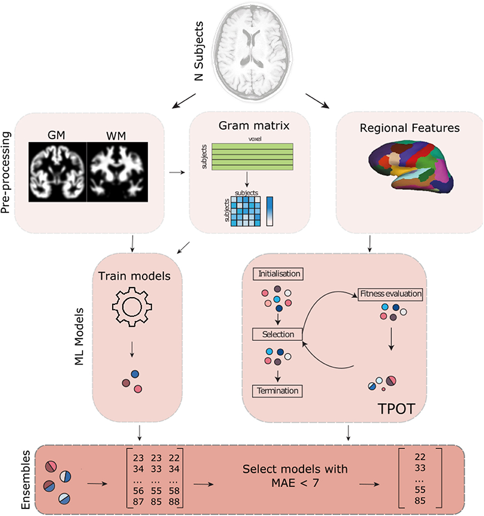
Figure 1. Overview of the different methods used in our analysis. In addition to the gray matter (GM) and white matter (WM) volume maps provided by the PAC competition, we also pre-processed the data in order to obtain the regional volume, thickness and mean curvature information of the brain using Freesurfer. We then used different strategies that involved creating a gram matrix, dimensionality reduction algorithms (e.g., PCA) and TPOT (an automated machine learning framework) to train different models. In addition, to using different pre-processing, we also trained different models for the different sites where the data was recorded. All models that had a mean absolute error (MAE) lower than 7 years were used to build a weighted ensemble.

2.1. Dataset

The data used in this analysis were derived from T1-weighted MRI images. All participants of the competition were provided with the raw NIfTI files as well as the pre-processed data (13). This dataset was acquired in 17 different sites that were not disclosed. The cohort used for training our algorithms consisted of N = 2, 640 healthy individuals (male/female = 1, 237/1, 403, mean age = 35.87±16.20, range 17−90). An independent test set (N = 660) was used to validate the performance of the model submitted by each participating team.

2.2. Pre-processing

2.2.1. Normalized Brain Volume Maps

The pre-processed normalized volume maps were already provided by the PAC 2019 organizers and were generated following the process described in (13). Briefly, this method consisted in segmenting gray matter (GM) and white matter (WM) volumetric maps using SPM12 (University College London, London, UK) according to their tissue classification. The normalization to the MNI152 was performed using DARTEL and a 4 mm Gaussian smoothing kernel. The size of the smoothing kernel was chosen to be the default value, which has been commonly used in previous research (12, 23). Lancaster et al. (24) explored the impact of voxel size and kernel size and observed that the values suggested by using Bayesian optimization are close to the values commonly used. To facilitate comprehension and inform the reader, we have briefly reported here how the WM and GM extraction was performed, however, we did not perform this step during our analysis. The only pre-processing that we have applied to the data was the FreeSurfer analysis, which has been described in the section below. We have used the WM and GM volumes that were provided by the PAC organizers. For our analysis we used a combination of GM, WM, and GM+WM maps as input for our models. All maps were acquired using all voxels and data were pre-processed in order to ensure that all images were brought into the same space for the appropriate machine learning analysis.

2.2.2. Brain Regional Features

We also extracted structural features using a surface-based approach implemented by FreeSurfer pipeline (v6.0). We obtained the estimations of the cortical thickness, volume, and mean curvature and anatomical structure volumes using the “recon-all” command [more detailed information about the processing in (25, 26)]. The cortical surface of each hemisphere was parcelated according to the Desikan-Killiany atlas (27). This process calculated the cortical thickness, volume, and mean curvature for each of the 68 brain regions (34 in each hemisphere) and volumes of the 45 anatomical structures (saved as stats/aseg.stats under the FreeSurfer subject directory).

2.3. Shallow Machine Learning Algorithms

Brain age has been a focus of research in the past few years, resulting in a rich literature on the topic (13, 28). Despite this, there is little agreement on which model performs best on brain data to predict age, mainly due to wide variations in methodologies and types of data. There are three classical machine learning models that are commonly used to predict brain age: Linear Regressors (LR), Support Vector Regressors (SVR), and Gaussian Process Regressors (GPR). Because of their popularity, in this work we trained these three models to predict brain age on the different types of data pre-processing previously described using K-fold cross-validation on the training set. The very large number of features made it computationally unfeasible to train the model directly on the brain volume maps. To overcome this limitation the pair-wise kernel matrix was pre-computed to reduce the dataset to an NxN matrix, where N refers to the number of data points, and was passed to the SVR models. As for the linear regressor model, the number of features in the dataset was reduced by Principal Component Analysis (PCA), by preserving 95% of the original variance of the dataset. This allowed to reduce the dimensions used by the models while still maintaining most of information. Besides training on the whole dataset, the models were also trained separately on each individual site, to adjust for the known problem of between-scanner variability (29). The main idea behind this is that by training all sites separately, every model will only learn biological features that are relevant to predict brain age and non-biological information (i.e., different scanner settings) or potential dataset biases cannot be learned by the model.

2.3.1. Linear Regression

LR is a simple parametric modeling approach that tries to model the relationship between the independent variables, X, and the target variable, y. It does so, by adapting the weights θ to fit a linear equation to the observed data. This modeling of the data has an analytical solution to obtain the optimal θ (Equation 1).

LR assumes that the relationship between the independent variables and the target variable is linear, which is a drawback from this model, as the brain data that serves as input is highly non-linear regarding the dependent variable, age (30). The main advantages of this modeling approach are its simplicity, transparency, and analytical solution (Equation A1).

2.3.2. Support Vector Regressor

SVR is a supervised learning model that fits a regression to the training data by minimizing the distance of the sampled points to a margin of tolerance around the fitted hyperplane (31). This is a sparse algorithm, which means it only requires the information of a small number of data points (i.e., support vectors) to define the hyperplane that is used for prediction of unseen data. This facilitates handling of datasets with a high number of data points. We mapped the original space into a kernel space by applying a pair-wise kernel function. By pre-computing the kernel space, we greatly reduce the computational resources spent training the model, as the number of variables is reduced to be the same size as the number of data points. We obtained the regularization hyperparameter C by using Grid-search over the search space of {2⁻⁶, 2⁻⁵, 2⁻⁴, 2⁻³, 2⁻², 2⁻¹, 2⁰, 2¹}. The hyperparameter C is used to reduce overfitting by virtue of a trade-off between the regression complexity and the precision of the model.

2.3.3. Gaussian Process Regressor

GPR is a non-parametric modeling approach that uses Bayesian inference to solve regression problems (32). It does so, by learning a probability distribution of possible target values based on a Gaussian process (GP) prior, which incorporates the prior knowledge of the space. The GP is specified using a mean function, 0 in this case, and a covariance function also called kernel. In this work we analyzed three different kernels: a pre-computed pair-wise kernel, Radial Basis Function kernel (RBF) and a white kernel. Because this modeling approach is not sparse, unlike the SVR, it is computationally burdensome, especially when dealing with high number of variables as is the case in voxel-based data. Due to resource limitations, the GPR was only trained on the surface-based morphometry data.

2.4. TPOT Models

TPOT [Tree-based Pipeline Optimization tool; (33), https://zenodo.org/record/3872281] is an open source framework that uses genetic programming to test multiple pipelines and find the most appropriated machine learning model for the problem at hand.

TPOT allows the user to define a pool of algorithms to be used. This pool of models can contain models that are pre-defined by TPOT or can include any model written by the user, or even be from any available package [e.g., the scikit-learn library; (34)] chosen by the user. The pool of models is not limited to machine learning algorithms but can include different pre-processing as well feature transformations algorithms. For this analysis we have included to the pool of models available to TPOT, not only the most popular algorithms to predict brain age (e.g., SVR, RVR, and GPR), but we also include other linear models (e.g., Lasso and Ridge Regression). To see a full list of the models used the reader can refer to Supplementary Table 1.

TPOT works by (i) selecting the algorithms from the user defined pool of algorithms, (ii) using with a cross-validation approach it trains those chosen algorithms and pass those with the highest accuracy to the next generations, (iii) the 20 pipelines with the best performance will be mutated/cross-over and passed to the next generation, (iv) once the last generation is reached (the number of generations is specified by the user before starting the analysis) the model with the highest accuracy and lowest complexity will be returned to the user. Therefore, together with the fact that TPOT allows the best model and parameter to be chosen in a data-driven fashion, one of its main advantages is that it penalizes overfitting by selecting the pipeline with the best performance but the lowest number of algorithms.

2.5. Ensemble

Ensembles of models tend to outperform single models and are a common technique to bolster algorithm's accuracy (35, 36). Ensembles tend to be more flexible in the functions they can represent, as they are not limited to a single hypothesis space of each model it is composed from. To perform a weighted ensemble, we used the mean absolute error (MAE) of each model on the K-fold cross validation. All models with a MAE above 7, our baseline, were discarded. The weight, w, given to a model's prediction was calculated by the squared difference between the baseline and the obtained MAE, in order to benefit smaller errors, following Equation 2. The weights were then used for a weighted average of the final prediction. For each site, only models trained on the site and on the whole training set were considered (Equation A2).

3. Results

The aim of our study was to develop pipelines that precisely predict the subject's age. To do this, we divided our analysis into two parts (i) we trained our pipelines using the data from all sites, (ii) we trained separate models for the 17 different sites. In addition, because different features might be more important for specific models, we also explored the effects of the different structural and regional features.

3.1. All Sites Analysis

Among the most used models to predict brain age, the SVR model trained with a combination of GM and WM achieved the best performance (MAE = 4.571 years; Table 1). These results are in line of those observed by (13) where they describe an increase in performance by combining both GM and WM information.

TABLE 1

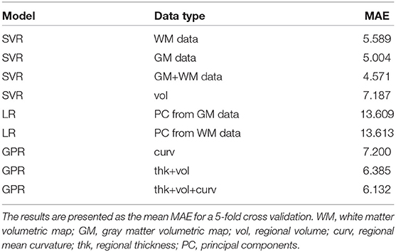
Table 1. Performance of each machine learning model when using the whole dataset.

On the other hand, when using TPOT and the regional features to find the most appropriate model, the returned pipeline consisted of a combination of linear regression and random forest regressor and yielded a MAE of 5.195 years.

3.2. Different Models for the Different Sites

To avoid non-biological variability induced by the different scanners, acquisition protocols and field strengths, we trained our best performing model from Table 1 (i.e., the SVR model which combined GM + WM information) using the data from each site separately. The performance of the site-specific models is reported in Table 2. The big oscillation in the MAE can be attributed to the difference in demographics of the different sites. As expected, the age-range per site correlated positively with the models' MAE (mean Pearson correlation coefficient across sites ± sd: 0.710 ± 0.001), as sites where participants had a small range of ages were easier to predict. Sample size per site had little correlation with the models' MAE (0.117 ± 0.656) and so did the sex ratio (0.147 ± 0.573).

TABLE 2

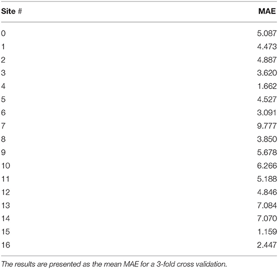
Table 2. Performance of the SVR model when using White Matter + Gray Matter volumetric data from each specific site.

Similarly, we also used the regional features to train TPOT in a site-specific fashion. In contrast to the results presented in Table 2 where we only used an SVR model and compared it's performance among the different sites, here we allowed TPOT to search for the best pipeline for each individual site (Table 3; to improve the readability here we only presented the models that composed the pipeline. If the reader is interested to know the models and their hyperparameters that lead to the optimal performance please see our Github—https://github.com/Mind-the-Pineapple/mind-the-gap). Interestingly, although none of the sites had the same pipeline the site-specific performance was in general comparable to that obtained when using only the SVR.

TABLE 3

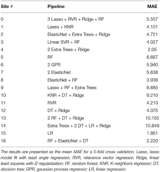
Table 3. Performance of the resulting TPOT pipelines when using thickness, volume, and mean curvature information from each specific site separately.

Finally, we combined the predictions of our models with a MAE <7 into an ensemble. To make sure that weakly performing models would not negatively impact our ensemble performance, we weighted the model's prediction on the ensemble based on its performance. In this weighted combination, we verified that none of the trained linear regressions performed well enough (their MAE was bigger than 7 years) to be included in the ensemble analysis, therefore we excluded any linear regression model from the ensemble. Models trained on individual sites were only considered for ensembles predicting data from their respective site. As different sites might have different scanners and other non-biological variations, by training each site separately every model learns the features that are relevant for brain-age prediction and its individual scanner properties and by keeping the sites independently it allows us to better account for inter-scanner variability. A crucial limitation that derives from this design choice is that the site information needs to be released together with the dataset. As this was the case for the PAC competition, we could use the subject's site information to choose the best model to predict brain age for that individual. Our ensemble had a mean absolute error of 3.7597 years on the independent test set, which was used to evaluate the performance of the different teams of the PAC 2019. To put this result into perspective, the best model, which consisted of an ensemble of computational intensive deep-learning models (37), achieved a performance of 2.9043 years on the same dataset.

4. Discussion

In this paper, we showed that shallow machine learning methods yield competitive results when predicting the brain age of the subjects from the PAC 2019 competition. In our approach, we used genetic-based methods and grid search to tune the hyperparameters of the different shallow models and trained the models using different structural measures. Importantly, we also trained different models for the different sites so that we could better account for scanner variability.

Deep learning's popularity is extending widely in various areas of research and is becoming a common tool in neuroscience. However, it is still an open question if brain images can profit from deep neural networks to learn the non-linearities from brain images with the current small datasets and a high number of features, while still being able to generalize to unseen datasets (21, 38, 39). This discussion arises from the fact that neural networks require more observations in order to learn complex patterns and significantly surpass the performance of classical shallow methods. Besides, if deep learning methods are not provided with sufficient data, they will be more prone to overfit and not generalize due to the large number of parameters in the models. To illustrate this problem, while ImageNet, one of the most commonly used datasets to train deep-learning models to classify natural images, contains about 14 million images, the UK Biobank, one of the biggest research consortia, currently provides 45,000 brain scans and aims to have 100,000 by 2050 (40).

Given that the dataset provided by the competition consisted of a large number of participants (N >1, 000), our results support the findings from (21). They showed that while for two benchmark datasets used in machine learning (i.e., MNIST and Zalando Fashion datasets) the performance of the deep-learning methods improved with an increase in the number of samples used to train the methods, that was not the case for linear models, where a plateau performance was reached. For neuroimaging datasets (i.e., volumes, connectivity, and slices) the performance of shallow models did not approach a plateau and had very similar performance as deep-learning models. Therefore, this suggests that even by using a larger dataset, the maximal performance of shallow models are not reached when using neuroimaging datasets. Similarly, He et al. (39) showed that kernel methods are as precise as neural networks when predicting behavior but have a lower computational cost. Some other noteworthy advantages of linear models and shallower models compared to deep neural networks are: (i) they are in general easier to interpret (22); (ii) they are less computationally intensive and can more quickly be trained, (iii) deep learning architectures are hard to adapt to the problem at interest, therefore, one of the biggest limitations of deep learning is to adapt previous architecture to the problem at hand. An appropriate adaptation requires vast experience from the practitioner; (iv) linear models can run in any computer and does not require GPU access.

One of the biggest challenges of machine learning is to find the appropriate hyperparameters for the model to be trained (41). Due to the large number of possible models, their hyperparameters and suitability for the problem at hand, finding the most appropriate combination can be a bewildering and computational intensive task. To address this issue, in this competition we used: (i) grid search strategy, which repeatedly performed the analysis over a set of pre-defined hyperparameters; (ii) a genetic-based method that was performed by TPOT in order to find the most appropriate model and its hyperparameters (i.e., taking into account both precision and complexity). Similarly, to the results reported by Dafflon et al. (42) and the no free lunch principle (43), we observed that there was not a single model that always had the best performance when predicting age (Table 3). The different models identified by TPOT for each site probably changed due to biological (i.e., age range, population heterogeneity) and non-biological factors (i.e., field strength and scanner manufacturer). As previous studies reported, these confounding variables have a significant influence on the performance of machine learning applications in neuroimaging data (44–46). Nevertheless, the combination of models suggested by TPOT leads to an improved performance that probably balances the strength and limitations of the single models by combining them into a pipeline. Another interesting feature of TPOT is that while searching for the best model, TPOT penalizes models that obtain a better performance due to overfitting. Despite the risk of overfitting of some of our site specific pipelines, due to the small sample size of some sites, the out-of-sample evaluation performed by the PAC committee with an independent dataset revealed a good performance.

In this paper, we have also taken into account the scanner where each data point originated from, building site-specific models, before combining them with models trained on all scanners. This was an effort to address the common issue of data variability between scanners, which can add variability in the dataset (47). For example, different scanner manufacturers, field strengths, or acquisition protocols which might have an effect on the algorithm's performance. One limitation of this site-specific approach is that some scanners have a small number of participants, resulting in models trained with low number of data points. To avoid overfitting to the sites, we discarded the models with poor performance (MAE>7). Another limitation of predicting age from brain images is the inter-variability and heterogeneity (i.e., different degrees of brain aging that might reflect different life styles, genetics, exclusion/inclusion criteria, and undiagnosed diseases) even in healthy participants, resulting in a noteworthy irreducible error in brain age prediction. In line with this idea, Holmes and Patrick (48) proposed that variability is also present in healthy controls and should be better addressed.

In conclusion, this paper shows that leveraging shallow models and ensemble learning to predict age from brain data is a simple but effective way of obtaining successful predictive models, despite the intrinsic non-linearity of the data. This approach also results in more interpretable models than deep learning models, as it is easier to deconstruct the model's mechanisms. Ultimately, this simple approach obtained a top-10 qualification in the PAC 2019 competition, competing directly with more complex and non-linear predictive models.

Data Availability Statement

The data analyzed in this study is subject to the following licenses/restrictions: The dataset is part of the Predictive Analytics Competition (PAC) 2019. Requests to access these datasets should be directed to Tim Hahn, Hahn_T@klinik.uni-wuerzburg.de.

Author Contributions

PD, JD, and WP designed and performed the experiments and wrote the manuscript. All authors contributed to the article and approved the submitted version.

Funding

WP was supported by the Wellcome Flagship Programme [WT213038/Z/18/Z].

Conflict of Interest

The authors declare that the research was conducted in the absence of any commercial or financial relationships that could be construed as a potential conflict of interest.

Supplementary Material

The Supplementary Material for this article can be found online at: https://www.frontiersin.org/articles/10.3389/fpsyt.2020.604478/full#supplementary-material

References

1. Deary IJ, Corley J, Gow AJ, Harris SE, Houlihan LM, Marioni RE, et al. Age-associated cognitive decline. Br Med Bull. (2009) 92:135–52. doi: 10.1093/bmb/ldp033

PubMed Abstract | CrossRef Full Text | Google Scholar

2. Grady C. The cognitive neuroscience of aging. Nat Rev Neurosci. (2012) 13:491–505. doi: 10.1038/nrn3256

PubMed Abstract | CrossRef Full Text | Google Scholar

3. Cole JH, Franke K, Cherbuin N. Quantification of the biological age of the brain using neuroimaging. In: Moskalev A, editor. Biomarkers of Human Aging. Cham: Springer (2019). p. 293–328. doi: 10.1007/978-3-030-24970-0_19

CrossRef Full Text | Google Scholar

4. Fjell AM, Walhovd KB. Structural brain changes in aging: courses, causes and cognitive consequences. Rev Neurosci. (2010) 21:187–221. doi: 10.1515/REVNEURO.2010.21.3.187

PubMed Abstract | CrossRef Full Text | Google Scholar

5. Fjell AM, McEvoy L, Holland D, Dale AM, Walhovd KB, Initiative ADN, et al. What is normal in normal aging? Effects of aging, amyloid and Alzheimer's disease on the cerebral cortex and the hippocampus. Prog Neurobiol. (2014) 117:20–40. doi: 10.1016/j.pneurobio.2014.02.004

PubMed Abstract | CrossRef Full Text | Google Scholar

6. Wyss-Coray T. Ageing, neurodegeneration and brain rejuvenation. Nature. (2016) 539:180–6. doi: 10.1038/nature20411

PubMed Abstract | CrossRef Full Text | Google Scholar

7. Convit A, Wolf OT, de Leon MJ, Patalinjug M, Kandil E, Caraos C, et al. Volumetric analysis of the pre-frontal regions: findings in aging and schizophrenia. Psychiatry Res. (2001) 107:61–73. doi: 10.1016/S0925-4927(01)00097-X

PubMed Abstract | CrossRef Full Text | Google Scholar

8. Becker BG, Klein T, Wachinger C, Initiative ADN. Gaussian process uncertainty in age estimation as a measure of brain abnormality. NeuroImage. (2018) 175:246–58. doi: 10.1016/j.neuroimage.2018.03.075

PubMed Abstract | CrossRef Full Text | Google Scholar

9. Liem F, Varoquaux G, Kynast J, Beyer F, Masouleh SK, Huntenburg JM, et al. Predicting brain-age from multimodal imaging data captures cognitive impairment. Neuroimage. (2017) 148:179–88. doi: 10.1016/j.neuroimage.2016.11.005

PubMed Abstract | CrossRef Full Text | Google Scholar

10. Valizadeh S, Hänggi J, Mérillat S, Jäncke L. Age prediction on the basis of brain anatomical measures. Hum Brain Mapp. (2017) 38:997–1008. doi: 10.1002/hbm.23434

PubMed Abstract | CrossRef Full Text | Google Scholar

11. Wang J, Li W, Miao W, Dai D, Hua J, He H. Age estimation using cortical surface pattern combining thickness with curvatures. Med Biol Eng Comput. (2014) 52:331–41. doi: 10.1007/s11517-013-1131-9

PubMed Abstract | CrossRef Full Text | Google Scholar

12. Cole JH, Leech R, Sharp DJ, Initiative ADN. Prediction of brain age suggests accelerated atrophy after traumatic brain injury. Ann Neurol. (2015) 77:571–81. doi: 10.1002/ana.24367

PubMed Abstract | CrossRef Full Text | Google Scholar

13. Cole JH, Poudel RPK, Tsagkrasoulis D, Caan MWA, Steves C, Spector TD, et al. Predicting brain age with deep learning from raw imaging data results in a reliable and heritable biomarker. Neuroimage. (2017) 163:115–24. doi: 10.1016/j.neuroimage.2017.07.059

PubMed Abstract | CrossRef Full Text | Google Scholar

14. Le TT, Kuplicki RT, McKinney BA, Yeh HW, Thompson WK, Paulus MP, et al. A nonlinear simulation framework supports adjusting for age when analyzing BrainAGE. Front Aging Neurosci. (2018) 10:317. doi: 10.3389/fnagi.2018.00317

PubMed Abstract | CrossRef Full Text | Google Scholar

15. Han LK, Dinga R, Hahn T, Ching CR, Eyler LT, Aftanas L, et al. Brain aging in major depressive disorder: results from the ENIGMA Major Depressive Disorder working group. Mol Psychiatry. (2020). doi: 10.1038/s41380-020-0754-0

PubMed Abstract | CrossRef Full Text | Google Scholar

16. Cole J, Raffel J, Friede T, Eshaghi A, Brownlee W, Chard D, et al. Accelerated brain aging and disability in multiple sclerosis. bioRxiv. (2019) 584888. doi: 10.1101/584888

CrossRef Full Text | Google Scholar

17. Cole JH, Raffel J, Friede T, Eshaghi A, Brownlee WJ, Chard D, et al. Longitudinal assessment of multiple sclerosis with the brain-age paradigm. Ann Neurol. (2020) 88:93–105. doi: 10.1002/ana.25746

PubMed Abstract | CrossRef Full Text | Google Scholar

18. Kaufmann T, van der Meer D, Doan NT, Schwarz E, Lund MJ, Agartz I, et al. Common brain disorders are associated with heritable patterns of apparent aging of the brain. Nat Neurosci. (2019) 22:1617–23. doi: 10.1038/s41593-019-0471-7

PubMed Abstract | CrossRef Full Text | Google Scholar

19. Schnack HG, Van Haren NE, Nieuwenhuis M, Hulshoff Pol HE, Cahn W, Kahn RS. Accelerated brain aging in schizophrenia: a longitudinal pattern recognition study. Am J Psychiatry. (2016) 173:607–16. doi: 10.1176/appi.ajp.2015.15070922

PubMed Abstract | CrossRef Full Text | Google Scholar

20. Franke K, Luders E, May A, Wilke M, Gaser C. Brain maturation: predicting individual BrainAGE in children and adolescents using structural MRI. Neuroimage. (2012) 63:1305–12. doi: 10.1016/j.neuroimage.2012.08.001

PubMed Abstract | CrossRef Full Text | Google Scholar

21. Schulz MA, Yeo BTT, Vogelstein JT, Mourao-Miranada J, Kather JN, Kording K, et al. Different scaling of linear models and deep learning in UKBiobank brain images versus machine-learning datasets. Nat Commun. (2020) 11:4238. doi: 10.1038/s41467-020-18037-z

PubMed Abstract | CrossRef Full Text | Google Scholar

22. LeCun Y, Bengio Y, Hinton G. Deep learning. Nature. (2015) 521:436–44. doi: 10.1038/nature14539

PubMed Abstract | CrossRef Full Text | Google Scholar

23. Cole JH, Franke K. Predicting age using neuroimaging: innovative brain aging biomarkers. Trends Neurosci. (2017) 40:681–90. doi: 10.1016/j.tins.2017.10.001

PubMed Abstract | CrossRef Full Text | Google Scholar

24. Lancaster J, Lorenz R, Leech R, Cole JH. Bayesian optimization for neuroimaging pre-processing in brain age classification and prediction. Front Aging Neurosci. (2018) 10:28. doi: 10.3389/fnagi.2018.00028

PubMed Abstract | CrossRef Full Text | Google Scholar

25. Fischl B, Salat DH, Busa E, Albert M, Dieterich M, Haselgrove C, et al. Whole brain segmentation: automated labeling of neuroanatomical structures in the human brain. Neuron. (2002) 33:341–55. doi: 10.1016/S0896-6273(02)00569-X

PubMed Abstract | CrossRef Full Text | Google Scholar

26. Fischl B. FreeSurfer. Neuroimage. (2012) 62:774–81. doi: 10.1016/j.neuroimage.2012.01.021

PubMed Abstract | CrossRef Full Text | Google Scholar

27. Desikan RS, Ségonne F, Fischl B, Quinn BT, Dickerson BC, Blacker D, et al. An automated labeling system for subdividing the human cerebral cortex on MRI scans into gyral based regions of interest. Neuroimage. (2006) 31:968–80. doi: 10.1016/j.neuroimage.2006.01.021

PubMed Abstract | CrossRef Full Text | Google Scholar

28. Jonsson BA, Bjornsdottir G, Thorgeirsson TE, Ellingsen LM, Walters GB, Gudbjartsson DF, et al. Brain age prediction using deep learning uncovers associated sequence variants. Nat Commun. (2019) 10:5409. doi: 10.1101/595801

PubMed Abstract | CrossRef Full Text | Google Scholar

29. Gradin V, Gountouna V-E, Waiter G, Ahearn TS, Brennan A, Condon B, et al. Between- and within-scanner variability in the CaliBrain study n-back cognitive task. Psychiatry Res. (2010) 184:86–95. doi: 10.1016/j.pscychresns.2010.08.010

PubMed Abstract | CrossRef Full Text | Google Scholar

30. Fjell AM, Westlye LT, Grydeland H, Amlien I, Espeseth T, Reinvang I, et al. Critical ages in the life course of the adult brain: nonlinear subcortical aging. Neurobiol Aging. (2013) 34:2239–47. doi: 10.1016/j.neurobiolaging.2013.04.006

PubMed Abstract | CrossRef Full Text | Google Scholar

31. Cortes C, Vapnik V. Support-vector networks. Mach Learn. (1995) 20:273–97. doi: 10.1007/BF00994018

CrossRef Full Text | Google Scholar

32. Rasmussen CE. Gaussian Processes in machine learning. Lect Notes Comput Sci. (2004) 3176:63–71. doi: 10.1007/978-3-540-28650-9_4

CrossRef Full Text | Google Scholar

33. Olson RS, Moore JH. TPOT: A tree-based pipeline optimization tool for automating machine learning. In: Hutter F, Kotthoff L, Vanschoren J, editors. Automated Machine Learning. Cham: Springer (2019). p. 151–60. doi: 10.1007/978-3-030-05318-5_8

CrossRef Full Text | Google Scholar

34. Pedregosa F, Varoquaux G, Gramfort A, Michel V, Thirion B, Grisel O, et al. Scikit-learn: machine learning in python. J Mach Learn Res. (2011) 12:2825–30.

Google Scholar

35. Lacoste A, Larochelle H, Marchand M, Laviolette F. Agnostic Bayesian learning of ensembles. In: 31st International Conference on Machine Learning Bejing: ICML. (2014).

Google Scholar

36. Opitz D, Maclin R. Popular ensemble methods: an empirical study. J Artif Intell Res. (1999) 11:169–98. doi: 10.1613/jair.614

CrossRef Full Text | Google Scholar

37. Peng H, Gong W, Beckmann CF, Vedaldi A, Smith SM. Accurate brain age prediction with lightweight deep neural networks. Med Image Anal. (2019) 68:101871. doi: 10.1016/j.media.2020.101871

PubMed Abstract | CrossRef Full Text | Google Scholar

38. Abrol A, Fu Z, Salman M, Silva R, Du Y, Plis S, et al. Hype versus hope: deep learning encodes more predictive and robust brain imaging representations than standard machine learning. bioRxiv. (2020). doi: 10.1101/2020.04.14.041582

CrossRef Full Text | Google Scholar

39. He T, Kong R, Holmes AJ, Nguyen M, Sabuncu MR, Eickhoff SB, et al. Deep neural networks and kernel regression achieve comparable accuracies for functional connectivity prediction of behavior and demographics. Neuroimage. (2020) 206:116276. doi: 10.1016/j.neuroimage.2019.116276

PubMed Abstract | CrossRef Full Text | Google Scholar

40. Sudlow C, Gallacher J, Allen N, Beral V, Burton P, Danesh J, et al. UK biobank: an open access resource for identifying the causes of a wide range of complex diseases of middle and old age. PLoS Med. (2015) 12:e1001779. doi: 10.1371/journal.pmed.1001779

PubMed Abstract | CrossRef Full Text | Google Scholar

41. Hutter F, Kotthoff L, Vanschoren J. Automated machine learning. In: The Springer Series on Challenges in Machine Learning. Cham: Springer International Publishing (2019). doi: 10.1007/978-3-030-05318-5

CrossRef Full Text | Google Scholar

42. Dafflon J, Pinaya WHL, Turkheimer F, Cole JH, Leech R, Harris MA, et al. An automated machine learning approach to predict brain age from cortical anatomical measures. Hum Brain Mapp. (2020) 41:3555–66. doi: 10.1002/hbm.25028

PubMed Abstract | CrossRef Full Text | Google Scholar

43. Wolpert DH, Macready WG. No free lunch theorems for optimization. IEEE Trans Evol Comput. (1997) 1:67–82. doi: 10.1109/4235.585893

CrossRef Full Text | Google Scholar

44. Linn KA, Gaonkar B, Doshi J, Davatzikos C, Shinohara RT. Addressing confounding in predictive models with an application to neuroimaging. Int J Biostat. (2016) 12:31–44. doi: 10.1515/ijb-2015-0030

CrossRef Full Text | Google Scholar

45. Glocker B, Robinson R, Castro DC, Dou Q, Konukoglu E. Machine learning with multi-site imaging data: an empirical study on the impact of scanner effects. arXiv [Preprint]. arXiv:191004597. (2019).

Google Scholar

46. Dinga R, Schmaal L, Penninx BW, Veltman DJ, Marquand AF. Controlling for effects of confounding variables on machine learning predictions. BioRxiv. (2020). doi: 10.1101/2020.08.17.255034

CrossRef Full Text | Google Scholar

47. Fortin JP, Cullen N, Sheline YI, Taylor WD, Aselcioglu I, Cook PA, et al. Harmonization of cortical thickness measurements across scanners and sites. Neuroimage. (2018) 167:104–20. doi: 10.1016/j.neuroimage.2017.11.024

CrossRef Full Text | Google Scholar

48. Holmes AJ, Patrick LM. The myth of optimality in clinical neuroscience. Trends Cogn Sci. (2018) 22:241–57. doi: 10.1016/j.tics.2017.12.006

CrossRef Full Text | Google Scholar

Appendix

$\begin{array}{l}\theta ={(X^T·X)}^{-1}·X^T·y(A1)\end{array}$

$\begin{array}{l}{w}_{model}={(7-MA{E}_{model})}^2(A2)\end{array}$