A two-leaf daily GPP model based on a rectangular hyperbolic model adjusted for air temperature and vegetation type

An accurate and easy-to-use gross primary productivity (GPP) model is essential for studying the spatial and temporal dynamics of the terrestrial carbon cycle on a global scale. Light use efficiency (LUE) models and process-based models are the two most commonly used approaches for GPP modeling. While LUE models are simpler and more user-friendly, process-based models often achieve higher accuracy due to their detailed structure. In this study, we introduce a new two-leaf GPP model (TL-RHM) with two expression forms at a daily temporal resolution. The TL-RHM is developed by temporally integrating a modified rectangular hyperbolic model that incorporates the effects of temperature variations on GPP across various vegetation types. The performance of the TL-RHM is evaluated using data from 21 CO₂ eddy-covariance flux sites, covering four vegetation types: evergreen needleleaf forest, deciduous broadleaf forest, grassland, and evergreen broadleaf forest. The results demonstrate that the daily GPP simulated by the TL-RHM agrees well with the measured GPP for both calibration and validation datasets across all four vegetation types. These findings highlight the potential of the TL-RHM to accurately simulate daily GPP with a relatively simple model structure, offering a valuable tool for long time-series GPP simulations at regional or global scales.

1 Introduction

Gross primary productivity (GPP) is a key component of the terrestrial carbon cycle (Sarkar et al., 2024; Marsh et al., 2025; Cheng et al., 2022; Mäkelä et al., 2008), and it is usually modeled using light use efficiency (LUE) models and process-based models at time steps of ranging from half hour, an hour, a day, 8 days, and a month. LUE models are commonly used for time steps of a day, 8 days, and a month (Law and Waring, 1994; Running et al., 2004; Yuan et al., 2014). These models have the advantages of simple model structure and high computation efficiency, which can be combined with remotely sensed data to perform large-scale GPP modeling. However, LUE models are insufficient in mechanism descriptions of biophysical and biological processes involved in photosynthesis because they are highly integrated in terms of time and space. From the perspective of time, these LUE models do not consider the effects of diurnal variations of meteorological variables to photosynthesis, and also they do not consider the effects of day-to-day variations of meteorological variables when multiday composites of GPP are computed. From the perspective of space, they are usually based on the big-leaf model, which does not separate canopy leaves into sunlit and shaded leaves. So these spatiotemporal characteristics of LUE models result in their limitations in GPP computation, especially for daily GPP modeling (Raczka et al., 2013; Wang et al., 2013).

Process-based models (PBMs) are considered to have the ability for accurate simulation of GPP. Most of them are based on Farquhar’s enzyme kinetic (EK) photosynthesis model (Farquhar et al., 1980) or its variants such as Baldocchi’s model (Baldocchi, 1994), which couples Farquhar’s model with the Ball–Woodrow–Berry (BWB) stomatal conductance model (Ball et al., 1987) to derive an instantaneous leaf-scale photosynthesis model. Although both Farquhar’s and Baldocchi’s models are instantaneous models, they are never run at a second time step but are often run at half-hourly or hourly time steps (Wang et al., 2001; Ju et al., 2006). In each step, the half-hourly or hourly averaged values of meteorological variables are inputted for GPP computation. The advantage of PBMs is that they are developed based on the mechanism of biophysical and biological processes. Therefore, simulation accuracies of GPP by PBMs are considered to be better than those by LUE models. However, the use of PBMs may be limited in large-scale and long time-series GPP simulations with high spatial resolution due to the complex model structures and small time steps. This is because measured half-hourly or hourly input data are unavailable at a global scale and interpolated data may result in some uncertainties.

In fact, there is another type of GPP model, the rectangular hyperbolic model (RHM), which is usually applied in temperature-controlled experiments (Pachepsky et al., 1996; Saito et al., 2005). Compared to the two groups of GPP models mentioned above, RHM is rarely used for long-term large-scale GPP modeling because its two parameters—quantum yield and maximum photosynthetic rate—vary temporally for different vegetation types. The use of fixed parameters of RHM under variable natural conditions can lead to errors in GPP calculations.

Above all, the commonly used models have some shortcomings in efficient and accurate GPP computation. But when studying the global terrestrial ecosystem carbon cycle, we often need to calculate GPP at large scales (regional or global), over long time series, and with high spatial resolution. Therefore, we urgently need an easy-to-use and efficient GPP model with high simulation accuracy. One possible way to solve the problem is temporal integration of instantaneous Baldocchi’s photosynthesis model with respect to time and space as Baldocchi’s model is based on Farquhar’s photosynthesis model and takes only meteorological data as inputs. The integration can be performed because most meteorological variables follow predictable diurnal courses over the course of a day. For example, radiation usually follows a sine function with a peak at solar noon (Kimball and Bellamy, 1986). However, an analytical solution for the integration of Baldocchi’s model with respect to time is difficult to accomplish due to the complexity of the equations (Wang et al., 2014a). In order to overcome this problem, we present an alternative way to integrate Baldocchi’s model by establishing a relationship between Baldocchi’s model and the rectangular hyperbolic model. First, we develop a temperature- and vegetation type-adapted rectangular hyperbolic model by linking it to Baldocchi’s photosynthesis model with high fidelity. Then, we integrate the modified rectangular hyperbolic model with respect to time to obtain a leaf-scale daily GPP model. Finally, we couple the daily GPP model with a two-leaf upscaling strategy to get a two-leaf daily GPP model with two expression forms, namely, TL-RHM_sine and TL-RHM_sinesine. Therefore, the objective of this study is to develop a new daily canopy-scale model for accurate and efficient GPP calculation. The model is of both photosynthesis mechanism and simple model structure, and it is expected to provide support for large-scale, long time-series, and high spatial resolution GPP simulation.

2 Materials and methods

2.1 Flux tower sites and data

The flux tower datasets used to calibrate and validate the new proposed model are acquired from the AmeriFlux website (http://ameriflux.ornl.gov) and the Canadian Carbon Program (CCP) website (http://fluxnet.ccrp.ec.gc.ca). Twenty-one sites covering evergreen needle leaf forest (ENF), deciduous broadleaf forest (DBF), grassland, and evergreen broadleaf forest (EBF) are selected. For each site, half-hourly global radiation or photosynthetically active radiation, relative humidity, air temperature, and CO₂ flux data, as well as some key datasets such as max LAI, can be used in the study. The half-hourly data associated with equipment failures have been gap-filled using the artificial neural network method (Papale and Valentini, 2003) or Barr’s gap-filling method (Barr et al., 2004). In order to obtain the inputs of a new daily model, the half-hourly measurements of radiation and GPP are summed to daily values, while the half-hourly measurements of air temperature are used to extract the maximum and minimum air temperatures during a day. Since the daily GPP is simulated for a whole year, the time-series LAI data are needed for time-series GPP modeling. For most of the sites, there are no measured time-series LAI data, but the measured maximum LAI data are available. So, the measured maximum LAI data are combined with the time-series MODIS LAI to obtain time-series LAI data as the model input. To evaluate the model performance with independent data, for each of the vegetation types, nearly half of the sites are used for model calibration, and the remaining sites are used for model validation (Table 1).

Table 1

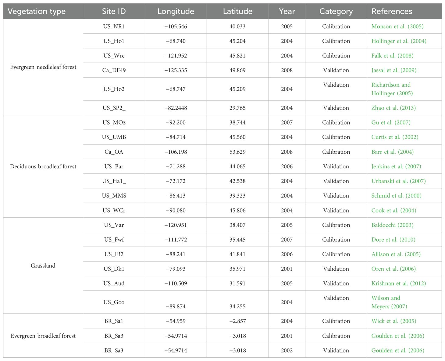
Table 1. The description of sites used in this study.

2.2 A leaf-scale temperature and vegetation type-adapted rectangular hyperbolic model

The traditional RHM can be expressed as Equation 1:

$\begin{array}{ll}GC{A}_{leaf}(t)=\frac{\alpha P_{m}APAR(t)}{P_m+\alpha APAR(t)}& (1)\end{array}$

where GCA_leaf is the leaf photosynthetic rate at time t, and α and P_m are the quantum yield and maximum photosynthetic rate at light saturation conditions, respectively.

The traditional RHM is usually applied in temperature-controlled experiments or over a few days during which temperature is assumed to be constant (Wang et al., 2014b). In our study, we improve the traditional RHM by establishing a relationship with Baldocchi’s photosynthesis model to obtain a modified RHM as follows: 1) for a given temperature and vegetation type, leaf-scale GPPs are modeled by Baldocchi’s photosynthesis model with a series of photosynthetic photon flux density (PPFD) values ranging from 50 μmol m⁻² s⁻¹ to 2,000 μmol m⁻² s⁻¹ as inputs; 2) the two parameters, α and P_m, are obtained by regressing PPFD against GPP using the rectangular hyperbolic model with fitted R² close to 1 (Supplementary Figure S1); and 3) the above two steps are repeated for all combinations of temperature from 1°C to 40°C and the maximum rate of Rubisco-mediated carboxylation (V_cmax,25) from 20 μmol m⁻² s⁻¹ to 180 μmol m⁻² s⁻¹ to get the α and P_m distribution maps (Ceccato et al., 2002) (see Supplementary Figures S2, S3). It should be pointed out that, for all combinations of temperature and V_cmax,25, the R² values of all fitted RHMs are greater than 0.99, meaning that, for a vegetation type, the modified RHM can perform as well as Baldocchi’s model under fixed temperature conditions (Wang et al., 2014a). The fact that RHM can accurately simulate the photosynthetic process under fixed temperature conditions has been proven in a previous study (Pachepsky et al., 1996). Therefore, we developed a leaf-scale RHM that is adjusted for air temperature and vegetation type, which is expressed as Equation 2:

$\begin{array}{ll}GC{A}_{leaf}(V_{\text{cmax},25},T,t)=\frac{\alpha (V_{\text{cmax},25},T)\times P_m(V_{\text{cmax},25},T)\times APAR(t)}{P_m(V_{\text{cmax},25},T)+\alpha (V_{\text{cmax},25},T)\times APAR(t)}& (2)\end{array}$

where GCA_leaf is the leaf-scale photosynthetic rate for a vegetation type with a fixed V_cmax,25 at a temperature T. α and P_m are the two parameters of GCA_leaf, and they are determined by temperature T and V_cmax,25.

2.3 Integration of the modified RHM with respect to time

The daily leaf-scale GCA can be calculated as:

$\begin{array}{ll}GC{A}_{daily,leaf}(V_{\text{cmax},25},T)={\displaystyle {\int }_{t_{rise}}^{t_{set}}\frac{\alpha (V_{\text{cmax},25},T_p)\times P_m(V_{\text{cmax},25},T_p)\times APAR(t)}{P_m(V_{\text{cmax},25},T_p)+\alpha (V_{\text{cmax},25},T_p)\times APAR(t)}}& (3)\end{array}$

where t_rise and t_set are the times of sunrise and sunset, respectively. T_p is the average temperature during the active photosynthesis period in the day.

The diurnal variation of APAR is described using a simple sine function (Kimball and Bellamy, 1986) or a squared sine function:

$\begin{array}{ll}APA{R}_t=APA{R}_{\text{noon}}\sin \left[\frac{\text{π(}t\text{ - }{t}_{\text{rise}})}{t_{\text{set}}-t_{\text{rise}}}\right]\text{ = }\frac{\text{π}APA{R}_{daily}}{2\text{Daylength}}\sin \left[\frac{\text{π(}t\text{ - }{t}_{\text{rise}})}{t_{\text{set}}-t_{\text{rise}}}\right]& (4)\end{array}$

$\begin{array}{ll}APA{R}_t=APA{R}_{\text{noon}}{\sin }^2\left[\frac{\text{π(}t\text{ - }{t}_{\text{rise}})}{t_{\text{set}}-t_{\text{rise}}}\right]\text{ = }\frac{2APA{R}_{daily}}{\text{Daylength}}{\sin }^2\left[\frac{\text{π(}t\text{ - }{t}_{\text{rise}})}{t_{\text{set}}-t_{\text{rise}}}\right]& (5)\end{array}$

Therefore, daily leaf-scale GPPs are expressed in the forms of Equations 6, 7 by substituting APAR in Equation 3 with Equation 4 or Equation 5. From Equation 4, we obtain the daily model (TL-RHM_sine).

$\begin{array}{ll}GP{P}_{daily}=\{\begin{array}{l}{P}_m\text{Daylength}\left[1-\frac{2a}{\pi \sqrt{a^2-1}}\left(\frac{\pi }{2}-\arctan \left(\frac{1}{\sqrt{a^2-1}}\right)\right)\right]a^2>1\\ P_m\text{Daylength}\left(1-\frac{\pi }{2}\right)a^2=1\\ P_m\text{Daylength}\left[1-\frac{a}{\pi \sqrt{a^2-1}}\ln \left(\frac{1+\sqrt{1-a^2}}{1-\sqrt{1-a^2}}\right)\right]a^2<1\end{array}& (6)\end{array}$

where Daylength is the length of day, $a=\frac{P_m}{\alpha APA{R}_{noon}}$, $APA{R}_{noon}=\frac{\pi APA{R}_{daily}}{2\text{Daylength}}$And from Equation 5, we obtain the daily model (TL-RHM_sinesine):

$\begin{array}{ll}GP{P}_{daily}=P_m\text{Daylength}\left(1-\sqrt{\frac{a}{a+1}}\right) & (7)\end{array}$

where Daylength is the length of day, $a=\frac{P_m}{\alpha APA{R}_{noon}}$, $APA{R}_{noon}=\frac{2APA{R}_{daily}}{\text{Daylength}}$

2.4 Upscaling leaf-scale GPP to canopy-scale using a two-leaf strategy

The canopy-scale GPP (GPP_canopy) can be calculated as the sum of the total GPP of sunlit and shaded leaves (Chen et al., 1999, 2012) (Equation 8):

$\begin{array}{ll}GP{P}_{\text{canopy}} = GC{A}_{\text{sunlit}}\times LA{I}_{\text{sunlit}}+GC{A}_{\text{shaded}}\times LA{I}_{\text{shaded}}& (8)\end{array}$

where the subscripts “sunlit” and “shaded” denote the sunlit and shaded components of GCA and leaf area index (LAI). The GCA_sunlit and GCA_shaded are calculated using Equations 6, 7. Moreover, the APAR of sunlit and shaded leaves and the total LAI separation into sunlit and shaded LAI are calculated using the methods of Chen et al. (1999). Therefore, the final daily canopy GPP models are the two two-leaf temperature and vegetation type-adapted rectangular hyperbolic models with the diurnal radiation following a sine function (Equation 4) and a squared sine function (Equation 5), called TL-RHM_sine and TL-RHM_sinesine, respectively. The inputs of the models are summarized in Supplementary Table S1.

Since the effect of relative humidity on GPP estimation is not considered in the new daily model, a scalar of vapor pressure deficit (VPD), f(VPD), is used to downregulate the daily GPP by TL-RHM under unfavorable conditions of high VPD (Equation 9), which will make the new daily model suitable for changeable environmental conditions.

$\begin{array}{ll}GP{P}_{\text{actual}}=GP{P}_{canopy}\times f(VPD)& (9)\end{array}$

where the GPP_actual is GPP regulated by VPD, and the f(VPD) can be expressed as follow (Equation 10):

$\begin{array}{ll}f(VPD)=\{\begin{array}{l}0\text{ VPD}\ge {\text{VPD}}_{\max }\\ \frac{VP{D}_{\max }-VPD}{VP{D}_{\max }-VP{D}_{\min }}{\text{ VPD}}_{\min }\le \text{VPD}\le {\text{VPD}}_{\max }\\ 1\text{ VPD}\le {\text{VPD}}_{\min }\end{array}& (10)\end{array}$

where VPD_max, VPD_min are the parameters dependent on vegetation types (Table 2).

Table 2

Table 2. Parameters calibrated for daily TL-RHM.

3 Results

The CO₂ eddy-covariance measurements from 21 sites with four vegetation types—ENF, DBF, grassland (GRA), and EBF (Table 1)—are used to evaluate the two-leaf rectangular hyperbolic model (TL-RHM) at daily temporal resolution. Since the two forms of TL-RHM correspond to different assumptions for diurnal radiation patterns, their performance in GPP simulations will also be evaluated with different vegetation types.

3.1 Calibration of the two-leaf rectangular hyperbolic model by measurements

The two-leaf rectangular hyperbolic model is calibrated by conducting ensemble runs in a range of V_cmax,25, and then the optimal V_cmax,25 is determined for each vegetation type. The calibration results are shown in Table 2. For the calibration dataset, the R² and RMSE between the modeled and measured GPP are computed for all four vegetation types, i.e., ENF, DBF, GRA, and EBF. As seen in Figure 1, the GPP values modeled by TL-RHM_sine are in good agreement with those of the measured GPP with R² values of 0.797, 0.871, and 0.944 for ENF, DBF, and GRA sites and with RMSE values of 1.619, 1.630, and 1.033 g C m⁻² day⁻¹ for ENF, DBF, and GRA sites, respectively. For the EBF site, the modeled and measured GPPs show a relatively poorer agreement with an R² value of 0.500. However, since the variation range of GPP is small for the tropical evergreen forest, TL-RHM performs acceptably well in tracing the seasonal variation of GPP with an RMSE of 1.212 g C m⁻² day⁻¹. The comparisons between the measured GPP and the modeled GPP by TL-RHM_sinesine follow a similar pattern for the four vegetation types with R² values of 0.804, 0.881, 0.944, and 0.481 (Figure 2) and RMSE values of 1.549, 1.465, 0.911, and 1.265 g C m⁻² day⁻¹ for the ENF, DBF, GRA, and EBF sites. From Figures 1, 2, it can be seen that the TL-RHM_sine and TL-RHM_sinesine can accurately simulate daily variations of GPP for the ENF, DBF, and GRA sites, and both show a relatively poor performance for EBF sites due to their small variations of GPP. Although there is a small difference between TL-RHM_sine and TL-RHM_sinesine, TL-RHM_sinesine performs slightly better than TL-RHM_sine for ENF and DBF sites, while for EBF sites, the reverse is true.

Figure 1

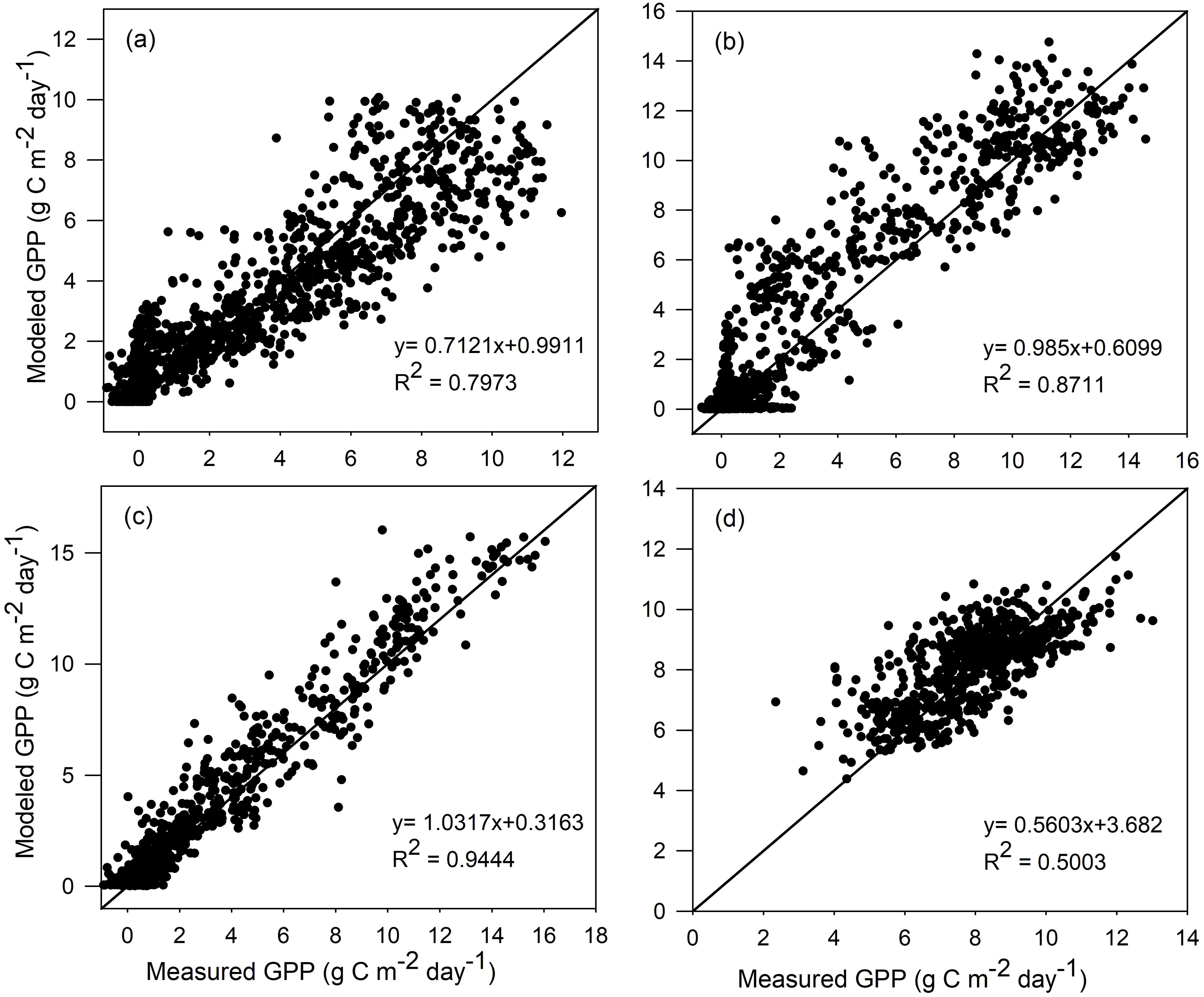
Figure 1. Scatterplots of GPP simulated by the TL-RHM_sine versus measured GPP for the calibration sites of (a) evergreen coniferous forest (three sites with 1,097 samples), (b) broadleaf deciduous forest (three sites with 1,097 samples), (c) grassland (three sites with 1,095 samples), and (d) evergreen broadleaf forest (two sites with 731 samples). Diagonal lines are the 1:1 lines.

Figure 2

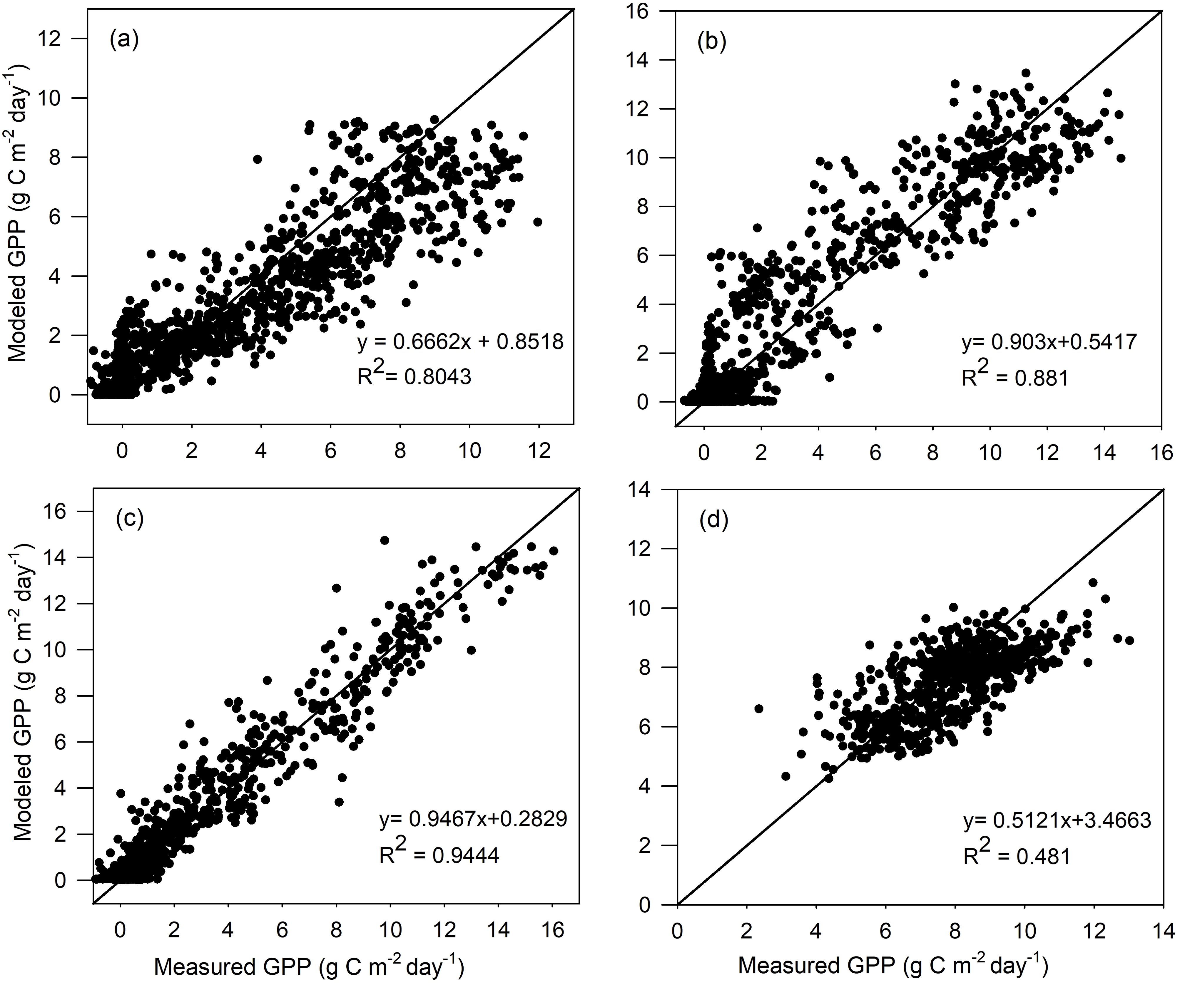
Figure 2. Scatterplots of GPP simulated by the TL-RHM_sinesine versus measured GPP for the calibration sites of (A) evergreen coniferous forest (three sites with 1,097 samples), (B) broadleaf deciduous forest (three sites with 1,097 samples), (C) grassland (three sites with 1,095 samples), and (D) evergreen broadleaf forest (two sites with 731 samples). Diagonal lines are the 1:1 lines.

For the calibration dataset, the modeled GPP by both TL-RHM_sine and TL-RHM_sinesine can track the seasonal variations of measured GPP for the four vegetation types. The modeled GPP also agrees well with day-to-day variations of measured daily GPP for most of the sites (Supplementary Figures S4–S7), but the two types of TL-RHM tend to overestimate GPP in the spring for the US_NR1 and US_Ho1 sites and are incapable of capturing the relatively high and low values of daily GPP for EBF sites.

3.2 Validation of the two-leaf rectangular hyperbolic model using measurements

The comparison results of the validation dataset are similar to those of the calibration dataset for the four vegetation types (Figures 3, 4). For TL-RHM_sine, the relatively large R² values of 0.725, 0.846, and 0.825 are obtained with RMSE values of 2.261, 1.916, and 1.349 g C m⁻² day⁻¹ for the ENF, DBF, and GRA sites, respectively. The R² for EBF sites is relatively small, similar to that of the calibration dataset, with an RMSE of 1.172 g C m⁻² day⁻¹. For TL-RHM_sinesine, the R² values between the modeled and measured GPPs are 0.732, 0.852, 0.826, and 0.463 with RMSE values of 2.001, 1.854, 1.214, and 1.230 g C m⁻² day⁻¹ for the ENF, DBF, GRA, and EBF sites, respectively. In Figures 3a, 4a, the points corresponding to the overestimation of GPP are mainly from Ca_DF49, that is because the V_cmax,25 for that site is lower than the average values of evergreen needleleaf forest.

Figure 3

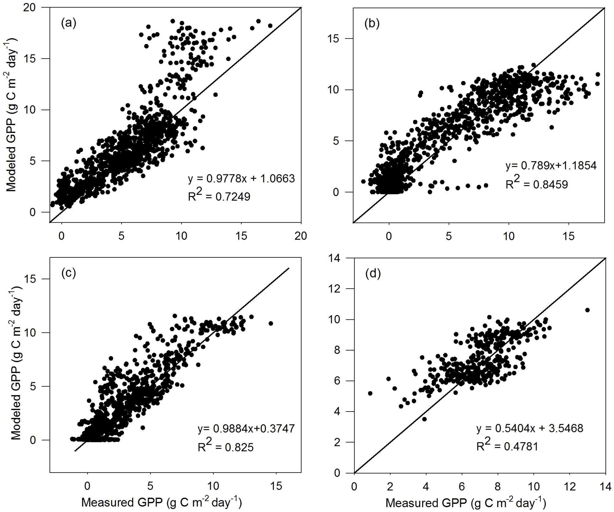
Figure 3. Scatterplots of GPP simulated by the TL-RHM_sine versus measured GPP for the validation sites of (a) evergreen coniferous forest (three sites with 1,098 samples), (b) broadleaf deciduous forest (four sites with 1,463 samples), (c) grassland (three sites with 1,096 samples), and (d) evergreen broadleaf forest (one site with 365 samples). Diagonal lines are the 1:1 lines.

Figure 4

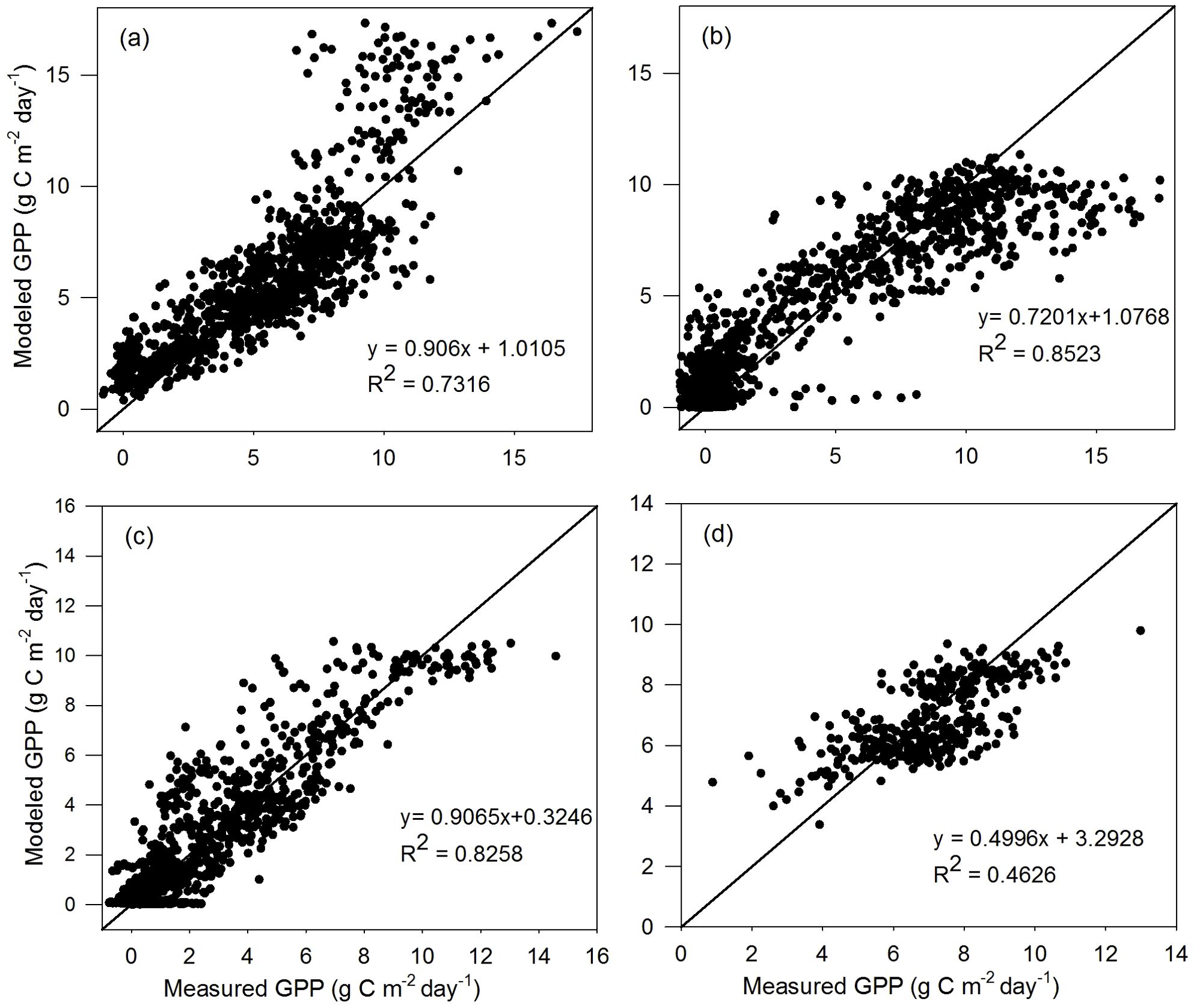
Figure 4. Scatterplots of GPP simulated by the TL-RHM_sinesine versus measured GPP for the validation sites of (a) evergreen coniferous forest (three sites with 1,098 samples), (b) broadleaf deciduous forest (four sites with 1,463 samples), (c) grassland (three sites with 1,096 samples), and (d) evergreen broadleaf forest (one site with 365 samples). Diagonal lines are the 1:1 lines.

For the validation dataset, the modeled GPP by both TL-RHM_sine and TL-RHM_sinesine can also track the seasonal variations of the measured GPP with a peak in summer for most of the ENF, DBF, and GRA sites and with a small significant seasonal change for the EBF site (Supplementary Figures S8–S11). The two types of TL-RHM can capture most of the low values of measured daily GPP during overcast days over the seasons but fail to capture the high values for the US_Ha1 site.

Although the GPPs simulated by the two types of TL-RHM show similar results for different vegetation types, the GPPs simulated by TL-RHM_sine are always greater than those by TL-RHM_sinesine for all sites, and the cause will be discussed in the discussion section. Moreover, the two types of TL-RHM behave differently in their simulation of daily GPP for different vegetation types. For the ENF, DBF, and GRA sites, the TL-RHM_sinesine performs slightly better than the TL-RHM_sine, while for the EBF sites, the TL-RHM_sine performs better.

4 Discussion

4.1 Comparison of the two types of daily TL-RHM

The difference between the two types of TL-RHM is the radiation function used in the daily integration with respect to time (Equations 4, 5). The maximum daily radiations simulated by a squared sine function used in TL-RHM_sinesine are always higher than those simulated by a sine function in TL-RHM_sine. This can be proven by deriving Equations 11, 12:

$\begin{array}{ll}\begin{array}{l}{R}_{\text{daily}}={\displaystyle {\int }_0^{\text{Daylength}}{R}_{\text{noon},\text{sine}}\sin \frac{\text{π}t}{\text{Daylength}}\text{ dt}}\\ \text{ = -}{R}_{\text{noon},\text{sine}}\frac{\text{Daylength}}{\text{π}} {\text{cos}\frac{\text{πt}}{\text{Daylength}}|}_0^{\text{Daylength}}\\ \text{ =}\frac{2\times R_{\text{noon},\text{sine}}\times \text{Daylength}}{\text{π}}\end{array}& (11)\end{array}$

Then, the radiation at noon for the sine function, $R_{\text{noon},\text{sine}}=\frac{\text{π}{R}_{daily}}{2\times \text{Daylength}}$.

$\begin{array}{ll}\begin{array}{l}{R}_{\text{daily}}={\displaystyle {\int }_0^{\text{Daylength}}{R}_{\text{noon},\text{sine}}{\sin }^2\frac{\text{π}t}{\text{Daylength}}\text{ dt}}\\ \text{ = }{R}_{\text{noon},\text{squared-sine}}\frac{\text{Daylength}}{\text{π}} {\left[\frac{\text{π}t}{2\times \text{Daylength}}-\frac{1}{2}\sin \frac{2\text{π}t}{\text{Daylength}}\right]|}_0^{\text{Daylength}}\\ \text{ =}\frac{ R_{\text{noon},\text{squared-sine}}\times \text{Daylength}}{2}\end{array}& (12)\end{array}$

The radiation at noon for the squared sine function, $R_{\text{noon},\text{squared-sine}}=\frac{2\times R_{\text{daily}}}{\text{Daylength}}$. Therefore, since 2 is greater than PI/2, we can draw a conclusion that R_{noon,squared-sine} is higher than R_noon,sine, but except around the noon hours, the radiation simulated by a sine function is higher than that simulated by a squared sine function. Because GPPs at noon hours on clear days usually approach an asymptote, the increase in radiation at those hours does not produce a significant increase in the corresponding GPP, while the increase in radiation at morning or afternoon hours will result in an obvious increase in the corresponding GPP. Therefore, the modeled GPPs by TL-RHM_sine are always higher than those obtained by TL-RHM_sinesine, as shown in Figure 5. For ENF, DBF, GRA, and EBF, the R² values of the fitted linear equations between GPPs from TL-RHM_sine and TL-RHM_sinesine are close to 1, indicating that the GPPs simulated from the two types of TL-RHM are highly correlated with each other. The slopes of the fitted linear equations between GPPs are 0.93, 0.91, 0.92, and 0.92, respectively, for ENF, DBF, GRA, and EBF, with an average slope value of 0.92.

Figure 5

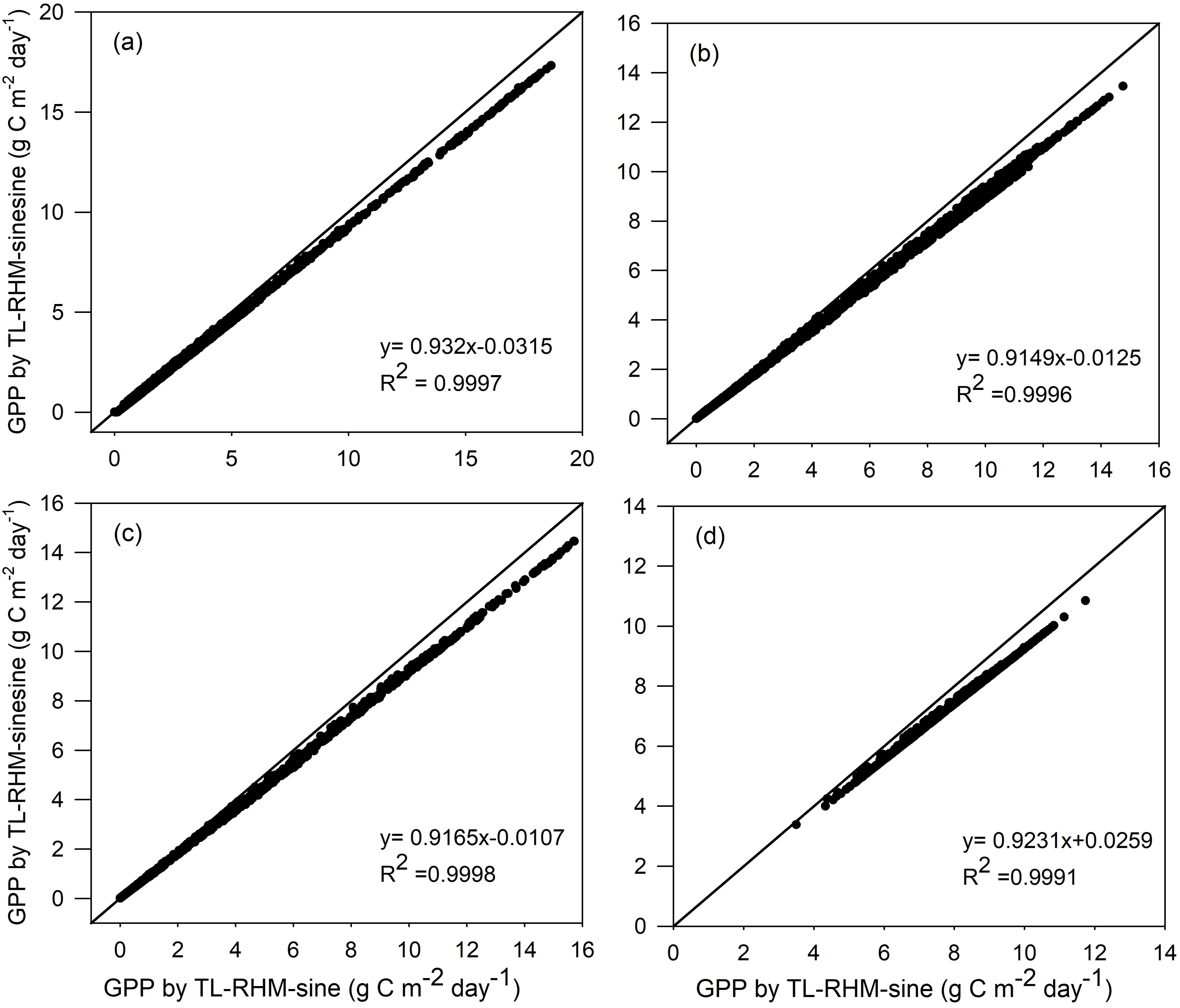
Figure 5. Comparisons of GPP simulated by the TL-RHM_sine and TL-RHM_sinesine for the sites of (a) evergreen coniferous forest, (b) broadleaf deciduous forest, (c) grassland, and (d) evergreen broadleaf forest. Diagonal lines are the 1:1 lines.

As to which type of TL-RHM performs better in GPP estimation, it depends on which radiation function (i.e., sine or squared sine) can accurately simulate the diurnal radiation variation at the study sites. In general, at high latitudes, solar radiation follows a squared sine function approximately, while it follows a sine function approximately at low latitudes. Therefore, TL-RHM_sine may be suitable for lower latitudes, while TL-RHM_sine may be appropriate for higher latitudes.

4.2 Limitations of daily TL-RHM

In the modified TL-RHM, we considered the effects of temperature and vegetation types on GPP. Although vapor pressure deficit was taken into account in the daily GPP estimation, it is only considered by an empirical function. Moreover, GPP is also affected by soil water content, but it is not included in daily TL-RHM. A possible solution is to introduce a soil water factor to the daily GPP model, similar to its application in LUE models. For large-scale applications, the water stress spectral index derived from remote sensing data can be used to downregulate daily GPP under conditions of deficient soil water content (Ceccato et al., 2002; Xiao et al., 2005). Finally, it should be noted that the influence of CO₂ concentration on photosynthesis is also not considered, but it is important for long-term GPP simulation. In addition, since the daily TL-RHM is developed based on Baldocchi’s photosynthesis model, the uncertainties in Baldocchi’s model may be inherited by the daily TL-RHM.

In our study, the diurnal variations of radiation were assumed to follow a sine or a squared sine function. The diurnal radiation basically follows a sine or a squared sine function. However, for an individual day, the assumption may not be satisfied under some unstable weather conditions (e.g., concurrent sunny and cloudy days in the morning or afternoon), in which the estimated daily GPP may not be accurately calculated by TL-RHM, and in most cases, overestimation of daily GPP may occur.

5 Conclusions

In our study, two types of daily two-leaf GPP models were developed. The two models called TL-RHMs were constructed by integrating a temperature and vegetation type-adapted rectangular hyperbolic model with respect to time to make them suitable for different environmental conditions and vegetation types. Four eddy-covariance measurement sites with different vegetation types and an hourly process model (the BEPS model) were used to evaluate the performance of the two types of the daily GPP model. Comparison results showed that the newly developed TL-RHMs can not only track the seasonal trends of daily GPP but also capture the day-to-day variation of daily GPP. The RMSE values between daily GPPs measured and simulated by TL-RHM_sine are 2.261, 1.916, and 1.349 g C m⁻² day⁻¹ for the ENF, DBF, and GRA sites, respectively, and 2.001, 1.854, 1.214, and 1.230 g C m⁻² day⁻¹ by TL-RHM_sinesine for the ENF, DBF, GRA and EBF sites, respectively. The results mean that TL-RHMs can simulate a comparative daily GPP as accurately as a process model but with a lower complexity compared to the TL-LUE model, indicating the great potential of TL-RHMs for daily GPP simulation at large scales.

Data availability statement

Publicly available datasets were analyzed in this study. This data can be found here: The flux tower data sets used to calibrate and validate the new proposed model are acquired from the AmeriFlux website (http://ameriflux.ornl.gov), and the Canadian Carbon Program (CCP) website (http://fluxnet.ccrp.ec.gc.ca).

Author contributions

QY: Formal analysis, Methodology, Software, Writing – original draft, Writing – review & editing, Conceptualization, Validation, Visualization. FW: Conceptualization, Formal analysis, Funding acquisition, Methodology, Supervision, Writing – review & editing.

Funding

The author(s) declare financial support was received for the research, authorship, and/or publication of this article. This study was supported by the Ningbo Key Research and Development Program (2022Z159) and the National Natural Science Foundation of China (42371328).

Acknowledgments

We thank the FLUXNET networks, the site principal investigators, co-investigators, participants, and data collection and processing staff for contributing to the tower flux data.

Conflict of interest

The authors declare that the research was conducted in the absence of any commercial or financial relationships that could be construed as a potential conflict of interest.

Generative AI statement

The author(s) declare that no Generative AI was used in the creation of this manuscript.

Publisher’s note

All claims expressed in this article are solely those of the authors and do not necessarily represent those of their affiliated organizations, or those of the publisher, the editors and the reviewers. Any product that may be evaluated in this article, or claim that may be made by its manufacturer, is not guaranteed or endorsed by the publisher.

Supplementary material

The Supplementary Material for this article can be found online at: https://www.frontiersin.org/articles/10.3389/fpls.2025.1555482/full#supplementary-material

References

Allison, V. J., Miller, R. M., Jastrow, J. D., Matamala, R., Zak, D. R. (2005). Changes in soil microbial community structure in a tallgrass prairie chronosequence. Soil Sci. Soc Am. J. 69, 1412–1421. doi: 10.2136/sssaj2004.0252

Crossref Full Text | Google Scholar

Baldocchi, D. (1994). An analytical solution for coupled leaf photosynthesis and stomatal conductance models. Tree Physiol. 14, 1069–1079. doi: 10.1093/treephys/14.7-8-9.1069

PubMed Abstract | Crossref Full Text | Google Scholar

Baldocchi, D. D. (2003). Assessing the eddy covariance technique for evaluating carbon dioxide exchange rates of ecosystems: Past, present and future. Global Change Biol. 9, 479–492. doi: 10.1046/j.1365-2486.2003.00629.x

Crossref Full Text | Google Scholar

Ball, J. W., Woodrow, I. E., Berry, J. A. (1987). “A model predicting stomatal conductance and its contribution to the control of photosynthesis under different environmental conditions,” in Progress in Photosynthesis Research. Ed. Biggins, J., Springer Nature Link. 221–224.

Google Scholar

Barr, A. G., Black, T. A., Hogg, E. H., Kljun, N., Morgenstern, K., Nesic, Z. (2004). Inter-annual variability in the leaf area index of a boreal aspenhazelnut forest in relation to net ecosystem production. Agric. For. Meteorol. 126, 237–255. doi: 10.1016/j.agrformet.2004.06.011

Crossref Full Text | Google Scholar

Ceccato, P., Gobron, N., Flasse, S., Pinty, B., Tarantola, S. (2002). Designing a spectral index to estimate vegetation water content from remote sensing data: Part 1 Theoretical approach. Remote Sens. Environ. 82, 188–197. doi: 10.1016/S0034-4257(02)00037-8

Crossref Full Text | Google Scholar

Chen, J. M., Liu, J., Cihlar, J., Goulden, M. L. (1999). Daily canopy photosynthesisy model through temporal and spatial scaling for remote sensing applications. Ecol. Model. 124, 99–119. doi: 10.1016/S0304-3800(99)00156-8

Crossref Full Text | Google Scholar

Chen, J. M., Mo, G., Pisek, J., Liu, J., Deng, F., Ishizawa, M., et al. (2012). Effects of foliage clumping on the estimation of global terrestrial gross primary productivity. Glob. Biogeochem. Cycle 26, GB1019. doi: 10.1029/2010GB003996

Crossref Full Text | Google Scholar

Cheng, E., Zhang, B., Peng, D., Zhong, L., Yu, L., Liu, Y., et al. (2022). Wheat yield estimation using remote sensing data based on machine learning approaches. Front. Plant Sci. 13. doi: 10.3389/fpls.2022.1090970

PubMed Abstract | Crossref Full Text | Google Scholar

Cook, B. D., Davis, K. J., Wang, W. G., Desai, A., Berger, B. W., Teclaw, R. M., et al. (2004). Carbon exchange and venting anomalies in an upland deciduous forest in northern Wisconsin, USA. Agric. For. Meteorol. 126, 271–295. doi: 10.1016/j.agrformet.2004.06.008

Crossref Full Text | Google Scholar

Curtis, P. S., Hanson, P. J., Bolstad, P., Barford, C., Randolph, J. C., Schmid, H. P., et al. (2002). Biometric and eddy-covariancebased estimates of annual carbon storage in five eastern North American deciduous forests. Agric. For. Meteorol. 113, 3–19. doi: 10.1016/S0168-1923(02)00099-0

Crossref Full Text | Google Scholar

Dore, S., Kolb, T. E., Montes-Helu, M., Eckert, S. E., Sullivan, B. W., Hungate, B., et al. (2010). Carbon and water fluxes from ponderosa pine forests disturbed by wildfire and thinning. Ecol. Appl. 20, 663–683. doi: 10.1890/09-0934.1

PubMed Abstract | Crossref Full Text | Google Scholar

Falk, M., Wharton, S., Schroeder, M., Ustin, S., Paw U, K. T. (2008). Flux partitioning in an old-growth forest: Seasonal and interannual dynamics. Tree Physiol. 28, 509–520. doi: 10.1093/treephys/28.4.509

PubMed Abstract | Crossref Full Text | Google Scholar

Farquhar, G. D., von Caemmerer, S., Berry, J. A. (1980). A biochemical model of photosynthetic CO2 assimilation in leaves of C3 species. Planta 149, 78–90. doi: 10.1007/BF00386231

PubMed Abstract | Crossref Full Text | Google Scholar

Goulden, M. L., Miller, S. D., da Rocha, H. R. (2006). Nocturnal cold air drainage and pooling in a tropical forest. J. Geophys. Res. 111, D08S04. doi: 10.1029/2005JD006037

Crossref Full Text | Google Scholar

Gu, L. H., Meyer, T., Pallardy, S. G., Hanson, P. J., Yang, B., Heuer, M., et al. (2007). Correction to influences of biomass heat and biochemical energy storages on the land surface fluxes and diurnal temperature range. J. Geophys. Res. 112, D02107. doi: 10.1029/2006JD007425

Crossref Full Text | Google Scholar

Hollinger, D. Y., Aber, J., Dail, B., Davidson, E. A., Goltz, S. M., Hughes, H., et al. (2004). Spatial and temporal variability in forest-atmosphere CO2 exchange. Glob. Change Biolo. 10, 1689–1706. doi: 10.1111/j.1365-2486.2004.00847.x

Crossref Full Text | Google Scholar

Jassal, R. S., Black, T. A., Spittlehouse, D. L., Brümmer, C., Nesic, Z. (2009). Evapotranspiration and water use efficiency in different-aged Pacific Northwest Douglas-fir stands. Agric. For. Meteorol. 149, 1168–1178. doi: 10.1016/j.agrformet.2009.02.004

Crossref Full Text | Google Scholar

Jenkins, J. P., Richardson, A. D., Braswell, B. H., Ollinger, S. V., Hollinger, D. Y., Smith, M. L. (2007). Refining light-use efficiency calculations for a deciduous forest canopy using simultaneous tower-based carbon flux and radiometric measurements. Agric. For. Meteorol. 143, 64–79. doi: 10.1016/j.agrformet.2006.11.008

Crossref Full Text | Google Scholar

Ju, W. M., Chen, J. M., Black, T. A., Barr, A. G., Liu, J., Chen, B. Z. (2006). Modelling multi-year coupled carbon and water fluxes in a boreal aspen forest. Agric. For. Meteorol. 140, 136–151. doi: 10.1016/j.agrformet.2006.08.008

Crossref Full Text | Google Scholar

Kimball, B. A., Bellamy, L. A. (1986). Generation of diurnal solar radiation, temperature, and humidity patterns. Energy Agric. 5, 185–197. doi: 10.1016/0167-5826(86)90018-5

Crossref Full Text | Google Scholar

Krishnan, P., Meyers, T. P., Scott, R. L., Kennedy, L., Heuer, M. (2012). Energy exchange and evapotranspiration over two temperate semi-arid grasslands in North America. Agric. For. Meteorol. 153, 31–44. doi: 10.1016/j.agrformet.2011.09.017

Crossref Full Text | Google Scholar

Law, B., Waring, R. (1994). Combining remote sensing and climatic data to estimatenet primary production across Oregon. Ecol. Appl. 4, 717–728. doi: 10.2307/1942002

Crossref Full Text | Google Scholar

Mäkelä, A., Pulkkinen, M. A., Kolari, P., Largergren, F., Berbigier, P., Lindroth, A., et al. (2008). Developing an empirical model of stand GPP with the LUE approach: Analysis of eddy covariance data at five contrasting conifer sites in Europe. Glob. Change Biolo. 14, 92–108. doi: 10.1111/j.1365-2486.2007.01463.x

Crossref Full Text | Google Scholar

Marsh, H., Jin, H. X., Duan, Z., Holst, J., Eklundh, L., Zhang, W. (2025). Plant Phenology Index leveraging over conventional vegetation indices to establish a new remote sensing benchmark of GPP for northern ecosystems. Int. J. Appl. Earth Obs. Geoinf. 136, 104289. doi: 10.1016/j.jag.2024.104289

Crossref Full Text | Google Scholar

Monson, R. K., Sparks, J. P., Rosenstiel, T. N., Scott-Denton, L. E., Huxman, T. E., Harley, P. C., et al. (2005). Climatic influences on net ecosystem CO2 exchange during the transition from wintertime carbon source to springtime carbon sink in a highelevation, subalpine forest. Oecologia 146, 130–147. doi: 10.1007/s00442-005-0169-2

PubMed Abstract | Crossref Full Text | Google Scholar

Oren, R., Hseih, C. I., Stoy, P., Albertson, J., McCarthy, H. R., Harrell, P., et al. (2006). Estimating the uncertainty in annual net ecosystem carbon exchange: Spatial variation in turbulent fluxes and sampling errors in eddy-covariance measurements. Global Change Biol. 12, 883–896. doi: 10.1111/j.1365-2486.2006.01131.x

Crossref Full Text | Google Scholar

Pachepsky, L. B., Haskett, J. D., Acock, B. (1996). An adequate model of photosynthesis—I. Parameterization, validation and comparison of models. Agric. Syst. 50, 209–225. doi: 10.1016/0308-521X(94)00051-R

Crossref Full Text | Google Scholar

Papale, D., Valentini, A. (2003). A new assessment of European forests carbon exchange by eddy fluxes and artificial neural network spatialization. Glob. Change Biol. 9, 525–535. doi: 10.1046/j.1365-2486.2003.00609.x

Crossref Full Text | Google Scholar

Raczka, B. M., Davis, K. J., Huntzinger, D., Neilson, R. P., Poulter, B., Richardson, A. D., et al. (2013). Evaluation of continental carbon cycle simulations with North American flux tower observations. Ecol. Monogr. 83, 531–556. doi: 10.1890/12-0893.1

Crossref Full Text | Google Scholar

Richardson, A. D., Hollinger, D. Y. (2005). Statistical modeling of ecosystem respiration using eddy covariance data: Maximum likelihood parameter estimation, and Monte Carlo simulation of model and parameter uncertainty, applied to three simple models. Agric. For. Meteorol. 131, 191–208. doi: 10.1016/j.agrformet.2005.05.008

Crossref Full Text | Google Scholar

Running, S. W., Nemani, R. R., Heinsch, F. A., Zhao, M. S., Reeves, M., Hashimoto, H. (2004). A continuous satellite-derived measure of global terrestrial primary production. BioSciences 54, 547–560. doi: 10.1641/0006-3568(2004)054[0547:ACSMOG]2.0.CO;2

Crossref Full Text | Google Scholar

Saito, M., Miyata, A., Nagai, H., Yamada, T. (2005). Seasonal variation of carbon dioxide exchange in rice paddy field in Japan. Agric. For. Meteorol. 135, 93–109. doi: 10.1016/j.agrformet.2005.10.007

Crossref Full Text | Google Scholar

Sarkar, D. P., Shankar, B. U., Parida, B. R. (2024). A novel approach for retrieving GPP of evergreen forest regions of India using random forest regression. Remote Sens. Appl: Soci. Environ. 33, 101116. doi: 10.1016/j.rsase.2023.101116

Crossref Full Text | Google Scholar

Schmid, H. P., Grimmond, C. S. B., Cropley, F., Offerle, B., Su, H. B. (2000). Measurements of CO2 and energy fluxes over a mixed hardwood forest in the mid-western United States. Agric. For. Meteorol. 103, 357–374. doi: 10.1016/S0168-1923(00)00140-4

Crossref Full Text | Google Scholar

Urbanski, S., Barford, C., Wofsy, S., Kucharik, C., Pyle, E., Budney, J., et al. (2007). Factors controlling CO2 exchange on timescales from hourly to decadal at Harvard Forest. J. Geophys. Res. 112, G02020. doi: 10.1029/2006JG000293

Crossref Full Text | Google Scholar

Wang, F. M., Chen, J. M., Gonsamo, A., Zhou, B., Cao, F. F., Yi, Q. X. (2014a). A two-leaf rectangular hyperbolic model for estimating GPP across vegetation types and climate conditions. J. Geophys. Res: Biogeosci. 119, 1385–1398. doi: 10.1002/2013JG002596

Crossref Full Text | Google Scholar

Wang, F. M., Gonsamo, A., Chen, J. M., Black, T. A., Zhou, B. (2014b). Instantaneous to daily GPP upscaling schemes based on a coupled photosynthesis−stomatal conductance model: correcting the overestimation of GPP by directly using daily average meteorological inputs. Oecologia 176, 703–714. doi: 10.1007/s00442-014-3059-7

PubMed Abstract | Crossref Full Text | Google Scholar

Wang, S., Grant, R. F., Verseghy, D. L., Black, T. A. (2001). Modelling plant carbon and nitrogen dynamics of a boreal aspen forest in CLASS – the Canadian Land Surface Scheme. Ecol. Model. 142, 135–154. doi: 10.1016/S0304-3800(01)00284-8

Crossref Full Text | Google Scholar

Wang, X. F., Ma, M. G., Li, X., Song, Y., Tan, J. L., Huang, G. H., et al. (2013). Validation of MODIS GPP product at 10 flux sites in northern China. Int. J. Remote Sens. 34, 587–599. doi: 10.1080/01431161.2012.715774

Crossref Full Text | Google Scholar

Wick, B., Veldkamp, E., de Mello, W. Z., Keller, M., Crill, P. (2005). Nitrous oxide fluxes and nitrogen cycling along a pasture chronosequence in Central Amazonia, Brazil. Biogeosci 2, 175–187. doi: 10.5194/bg-2-175-2005

Crossref Full Text | Google Scholar

Wilson, T. B., Meyers, T. P. (2007). Determining vegetation indices from solar and photosynthetically active radiation fluxes. Agric. For. Meteorol. 144, 160–179. doi: 10.1016/j.agrformet.2007.04.001

Crossref Full Text | Google Scholar

Xiao, X. M., Zhang, Q. Y., Hollinger, D., Aber, J., Moore, B. (2005). Modeling gross primary production of an evergreen needleleaf forest using MODIS and climate data. Ecol. Appl. 15, 954–969. doi: 10.1890/04-0470

Crossref Full Text | Google Scholar

Yuan, W. P., Cai, W. W., Xia, J. Z., Chen, J. Q., Liu, S. G., Dong, W. J., et al. (2014). Global comparison of light use efficiency models for simulating terrestrial vegetation gross primary production based on the LaThuile database. Agric. For. Meteorol. 192–193, 108–120. doi: 10.1016/j.agrformet.2014.03.007

Crossref Full Text | Google Scholar

Zhao, L., Lee, X., Liu, S. (2013). Correcting surface solar radiation of two data assimilation systems against FLUXNET observations in North America. J. Geophys. Res.: Atmos. 118, 9552–9564. doi: 10.1002/jgrd.50697

Crossref Full Text | Google Scholar