 Kang Xu
 Jiejie Xing
 Wenbin Sun1
- 1College of Information and Communication Engineering, Hainan University, Haikou, China
- 2College of Mechanical and Electrical Engineering, Hainan University, Haikou, China
Currently, precise spraying of sweet potatoes is mainly accomplished through semi-mechanized or single spraying robots, which results in low operating efficiency. Moreover, it is time-consuming and labor-intensive, and the pests and diseases cannot be eliminated in time. Based on multi robot navigation technology, multiple robots can work simultaneously, improving work efficiency. One of the main challenges faced by multi robot navigation technology is to develop a safe and robust collision avoidance strategy, so that each robot can safely and efficiently navigate from its starting position to the expected target. In this article, we propose a low-cost multi-robot collision avoidance method to solve the problem that multiple robots are prone to collision when working in field at the same time. This method has achieved good results in simulation. In particular, our collision avoidance method predicts the possibility of collision based on the robot’s position and environmental information, and changes the robot’s path in advance, instead of waiting for the robot to make a collision avoidance decision when it is closer. Finally, we demonstrate that a multi-robot collision avoidance approach provides an excellent solution for safe and effective autonomous navigation of a single robot working in complex sweet potato fields. Our collision avoidance method allows the robot to move forward effectively in the field without getting stuck. More importantly, this method does not require expensive hardware and computing power, nor does it require tedious parameter tuning.
1 Introduction
Sweet potato is an important food crop after rice, wheat, and corn. With the development of large-scale sweet potato cultivation, sweet potato diseases and pests are becoming increasingly serious. Traditional prevention and treatment methods are high in cost and low in efficiency, and there are problems such as prevention and treatment of chemical abuse and overuse. Harmful pesticide chemicals will spread into the air, causing pollution to the environment and sweet potato crops, and may enter farmers’ bodies through the respiratory system (Meshram et al., 2022). Precision spraying technology can solve the problems of pesticide waste and overuse, improve pesticide utilization, and reduce pesticide pollution to the environment (Xiongkui, 2020). However, in the current precision spraying operations, a single robot is mainly used for spraying operations, such as Danton et al., 2020; Baltazar et al., 2021; Oberti and Schmilovitch, 2021, and Liu et al., 2022. A single robot has the disadvantages of limited operating capacity and long operating time. Especially for sweet potato fields with a relatively large area, using a single robot for spraying will take a lot of time (Kim and Son, 2020), and pests and diseases cannot be eliminated in time, causing irreparable economic losses to agriculture. In addition, if the robot fails, the entire spraying operation will be delayed, resulting in greater economic losses. Therefore, applying a multi-robot system to sweet potato spraying can effectively solve the problem of low operating efficiency of a single device, reduce agricultural maintenance costs, and indirectly improve agricultural economic benefits. There are many benefits to using a multi-robot system instead of a single robot (Parker et al., 2016; Jawhar et al., 2018): (1) Multiple robots can perform tasks simultaneously to complete tasks faster. (2) Multiple robots can effectively handle tasks that are essentially distributed over a wide area. (3) When any robot fails, multiple robots that can perform similar processes can be used to compensate.
As the number of agricultural workers continues to decrease around the world, the use of multi-robot systems to perform agricultural tasks has become increasingly common in large-scale fields with fewer people (Carbone et al., 2018), and multi-robot systems have gradually become a hot topic of research. However, one of the main challenges facing multi-robot systems is to develop a safe and robust collision avoidance strategy that enables each robot to navigate safely and efficiently from the starting position to the desired target (Long et al., 2017). The robot’s obstacle avoidance method can be divided into local obstacle avoidance and global path according to the operation requirements (Tang et al., 2024), such as Genetic algorithm (Zhao et al., 2021), dynamic window approach (Chang et al., 2021), RRT* (Hu et al., 2024), A* (Zhang et al., 2024) and other algorithms. However, these obstacle avoidance methods are all for a single robot and are not suitable for multi-robot systems (Cai et al., 2007). At present, the collision avoidance methods of multi-robots are mainly divided into centralized control and decentralized control.
Initially, scholars used a centralized control method to avoid collisions between multiple robots. This approach assumed that the behavior of all robots was determined by a central controller that had comprehensive knowledge of all robots’ intentions (e.g., initial states and goals) and their workspaces (e.g., 2D grid maps). Schwartz and Sharir (1983) proposed to find the continuous motion of two given structures connecting objects within a given region, during which they avoided collisions with walls and each other. He et al. (2016) used the cloud platform to calculate local collision-free paths for each robot, which improved the processing capabilities of the device. However, this method needed to ensure that each robot had networking capabilities. Yu and LaValle (2016); Tang et al. (2018); Matoui et al. (2020) and Cheng et al. (2023) proposed a centralized trajectory generation algorithm to find trajectories that navigate robots from starting positions to non-interchangeable target positions in a collision-free manner by planning optimal paths for all robots. In addition, Keshmiri and Payandeh (2009) used a centralized method to keep multiple robots in formation to avoid collisions between robots, but it was not suitable for the agricultural field and cannot control multiple robots to maintain formation during precise spraying. Centralized approaches can ensure multi-robot system safety, integrity, and near-optimality, but they are difficult to scale to large systems with many robots due to the high computational cost of multi-robot scheduling, heavy reliance on reliable synchronous communication, and low tolerance for failures or interference.
Compared with centralized methods, some existing studies proposed decentralized collision avoidance strategies, where each robot made decisions independently by considering the observable states (such as shape, speed, and position) of other robots. Cai et al. (2007) developed an advanced method for collision avoidance in multi-robot systems based on established techniques of omnidirectional vision systems, automatic control, and dynamic programming. However, each robot in this system must be an autonomous robot, equipped with equipment or systems such as omnidirectional vision systems, target recognition systems, communication systems, and control systems. Claes et al. (2012); Hennes et al. (2012), and Godoy et al. (2016) designed inter-agent communication protocols to share position and velocity information among nearby agents. However, communication systems posed additional difficulties, such as delays or blocking of communication signals due to obstruction by obstacles. Althoff et al. (2012) proposed a probabilistic threat assessment method for reasoning about the safety of robot trajectories. In this method, the trajectories of other dynamic obstacles needed to be sampled and then the global collision probability was calculated. Lacked of possibilities for safe navigation in dynamic multi-robot environments. Sun et al. (2014) proposed a behavior-based multi-robot collision avoidance method in large robot teams inspired by the concept of swarm intelligence, which could solve the coordination problem of multi-robots by using group behavior. Fiorini and Shiller (1998), Van den Berg et al. (2008); Snape et al. (2009); Hennes et al. (2012); Alonso-Mora et al. (2013); Claes and Tuyls (2018), and Zhu et al. (2020) designed a robot collision avoidance strategy based on the speed obstacle framework. This algorithm effectively inferred the local collision-free motion of multiple agents in a chaotic workspace. However, these methods have several serious limitations that hinder their widespread application in practical scenarios. First of all, it is difficult to meet the requirement that each agent has perfect perception of the surrounding environment. This requirement does not hold true in real scenarios. A second limitation is that speed barrier-based strategies are controlled by multiple adjustable parameters that are sensitive to scene settings and therefore must be set carefully to achieve satisfactory multi-robot locomotion.
Inspired by methods based on the speed obstacle framework, Chen et al. (2017b), and Chen et al. (2017a) trained a collision avoidance strategy using deep reinforcement learning. This strategy explicitly mapped the agent’s own state and that of its neighbors to collision-free actions, but it still required perfect awareness of the surrounding environment. Long et al. (2017); Pfeiffer et al. (2017); Wang et al. (2020); Huang et al. (2022); Xiao et al. (2022), and Han et al. (2022) used deep neural network modeling and trained using supervised learning on large datasets. However, there are several limitations to supervised learning policies. First, it requires a large amount of training data, which should cover different interaction situations of multiple robots, and the training time cost is high. Secondly, the expert trajectories in the data set are not guaranteed to be optimal in interactive scenarios, which makes it difficult for training to converge to a robust solution. Third, it is difficult to manually design a suitable loss function to train a robust collision avoidance strategy. Fourth, the hardware requirements required for model deployment on robots are relatively high. When the number of robots increases, the hardware cost increases exponentially. Multi-robot systems based on reinforcement learning or transfer learning require a large amount of data sets for training, which requires relatively high time and economic costs. However, the economic benefits obtained in agriculture are obviously not suitable for the large-scale application of such robots.
Ünal et al. (2023) proposed a robot collision avoidance algorithm for traveling along tangent paths to solve the problem of multi-robot collision avoidance in precision agriculture. However, they only considered two robots and did not introduce the specific application environment. In addition, they did not consider whether the robot would damage the surrounding crops when avoiding collision. Currently, research on multi-robot collision avoidance strategies mainly focuses on confined space scenes or in relatively open and empty spaces, and no scholars have considered how to avoid collisions among multi-robots in large field (Raibail et al., 2022). Due to the special field environment, the robot can only move along the ridges, and can only move forward or backward. It cannot move freely in all directions, otherwise it will damage the crops and the robot, causing unnecessary economic losses. The current multi-robot collision avoidance strategy cannot be directly applied to this situation. In order to overcome the shortcomings of the above method, we propose a low-cost multi-robot collision avoidance method, which uses position and known environmental information to predict the possibility of collision, and changes the robot path in advance to achieve the purpose of robot collision avoidance. The method outperforms existing agent- and sensor-level methods in terms of navigation speed and safety. It can be directly and smoothly deployed on physical robots, without the need for expensive laser radars, cameras, and terminal controllers, and without the need for cumbersome parameter adjustments. Based on this, we propose a multi-robot collision-free method suitable for the special environment of field. The main innovations and contributions are as follows:
1. The multi-robot collision avoidance method we proposed only requires the robot to have a communication module, a positioning module and a low-cost control chip. It does not require the robot to have vision, radar and other sensors, nor does it require the ability to deploy reinforcement learning models. Reduce farmers’ purchase costs and field maintenance costs, thereby increasing farmers’ economic income.
2. We proposed a rapid robot path generation method suitable for farmland. The global information of the farmland was generated through the two endpoints of the crop rows and the row spacing. The global information included the straight-line equation and the two endpoints of the crop rows, occupying very little storage space. Then based on the requirements of farm operations and the robot’s target location, we could quickly generate a global path for the robot.
3. We proposed a robot collision avoidance method that could determine its own direction and working status only based on global information and the robot’s position. Then the robot’s position and global information were used to predict the possibility of collision in advance. Finally, the robot’s local path was adjusted according to the robot’s priority to avoid collisions. This method could quickly find collision-free paths for multi-robot systems and can be safely generalized to other work scenarios.
The rest of this paper is as follows: Section 2 introduces the working environment of multi-robot systems, related definitions and collision types. In Section 3, we discussed in detail how to predict the possibility of robot collision through maps and robot positions, and how to adjust local paths in the special environment of field to avoid collisions among multiple robots. The fourth section introduces the simulation environment and simulation settings of the multi-robot collision avoidance method, and verifies the method proposed in the third section. The final section presents the summary and prospects of this study.
2 Materials and methods
2.1 The working environment of robots
The sweet potato field is simplified to facilitate the description of the robot’s working conditions, as shown in Figure 1. The rectangle represents the field, and represents the working robots (Figure 1A). The line segments , , and represent the robot’s paths in the field (Figure 1B). The line segment is called the working path, the points and are the endpoints of the , respectively, and is the serial number of the working path. Line segments and are called the transition path. We set the sweet potato field to be planted in a standardized manner, with working paths running parallel to each other. The distance between each working path is represented by .
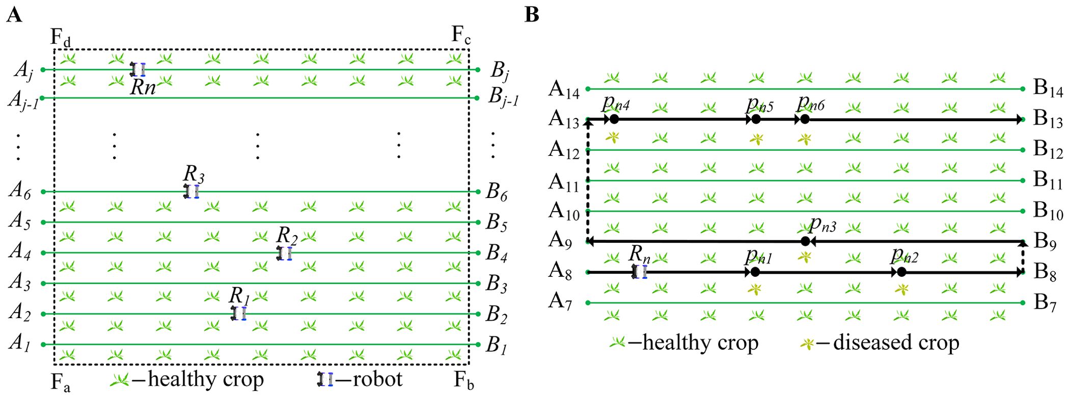
Figure 1. A simplified diagram of the robot’s working environment. (A) Simplified diagram of field. (B) The working path of the robot.
2.1.1 Definitions of robots
represents a group of working robots, as shown in Equation 1. has the same dynamic model in vertical and horizontal dimensions. The real-time location of is represented by , and is represented by coordinates .
represents other robots except for , as shown in Equation 2.
A group of target points of robot is represented by , as shown in Equation 3. Robot moves at a constant speed along the target point. After robot reaches target , it stops for 3 seconds and performs precision spraying operations.
where the coordinates of are represented by , and and are the horizontal and vertical coordinates on a two-dimensional plane, respectively. represents the global path of the robot, and represents the local path of the robot, as shown in Equation 4. The local path comprises a series of points, such as and , as shown in the solid black line in Figure 1B. comprises a series of local paths, such as all-black paths in Figure 1B.
There are two types of paths: the working and transition. In Figure 1B, the solid black lines , , and are the working path, and the dotted black lines and are the transition path.
The robot has different moving directions on the working and transition paths. When the robot is moving on the working path, the robot’s direction at points and are 0 and 1, respectively. When going from point to , the direction of the robot is . When the robot goes from point to , the robot’s direction is . Therefore, we can get the direction of the robot only through the two endpoints of the local path without using other sensors. The expression method of the robot’s moving direction in the working path is shown in Equation 5.
When the robot moves on the transition path, the direction is determined according to the serial number of the current and last working paths, as shown in Equation 6. The robot’s direction is when the is a positive number. When the is negative, the direction of the robot is . The direction on the transition path is only judged by the , and no other sensors are needed.
where represents the serial number of the current working path, and represents the serial number of the last working path.
2.1.2 The working rules of robots
The width of the working path in the field is relatively narrow, and it does not support operations such as moving side by side or turning; otherwise, the robots will crush or knock down the crops. Therefore, robots with different moving directions cannot simultaneously exist in the working path ; otherwise, the robots will collide.
The robots move in a ‘U’ shape in the field (Hameed et al., 2013), and the working method is shown in the black path in Figure 1B. For example, starts from point , moves along the working path , reaches the end point , and moves along to . In addition, robots start from the garage, go to the field to work, and then return to the garage.
2.2 Collision and conflict scenarios of robots
During the research, we found that the possibility of a robot collision can be judged based on the robot’s path type. When robots move on the same path type, we can determine whether the robots will collide by simply comparing their serial number of the working paths and directions. The path type and serial number are the same, indicating that they are in the same working path. At this time, if they are moving in opposite directions, it means that they are moving toward each other and a collision will inevitably occur. If they are moving in the same direction, as long as their speeds are the same, there will be no collision. Therefore, we divide the robot collision scenarios into four types based on the different positions of and : 1) working path and different movement directions; 2) working path and same movement direction; 3) transition path and same movement direction; 4) transition path and different movement directions.
As shown in Figure 2, it describes the possibility of collision when the robot is working. The green line segments represent the working paths, and the two working robots are represented by and ; their target points are and .
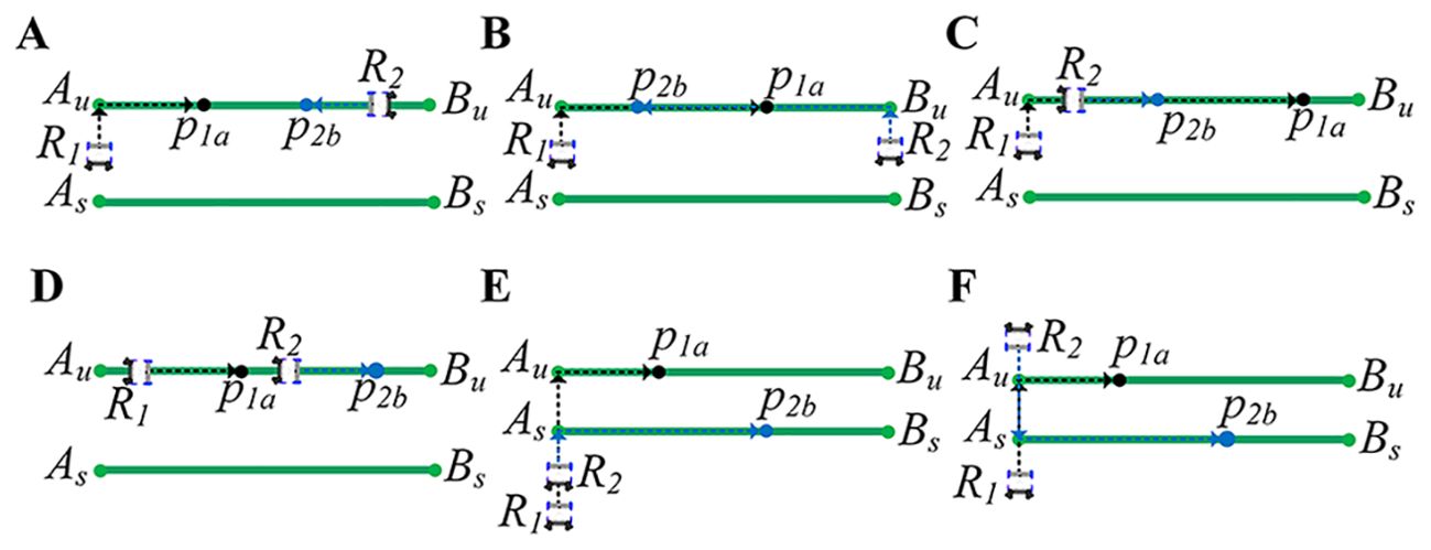
Figure 2. Types of robot conflicts. (A, B) Working path and different movement directions. (C, D) Working path and same movement direction. (E) Transition path and same movement direction. (F) Transition path and different movement directions.
2.2.1 Working path and different movement directions
Figure 2A describes that robot has been moving in the working path , and robot is about to enter the working path . Robots and move in opposite directions. According to section 2.1, there cannot be two robots with different moving directions in the same working path. If robot continues to enter the working path without changing its path, it will inevitably collide with .
Figure 2B describes that and are about to enter the same working path . Robots and are moving in opposite directions. If the path of robot or is not changed, and will eventually collide together.
2.2.2 Working path and same movement direction
Figure 2C describes that robot is already moving in the working path , and robot is about to enter the working path . Figure 2D describes that the robots and are already moving in the working path . Robots and move in the same direction. According to Section 2.1, two arobots with the same moving direction can exist in the same working path. Since the speeds of the robots are the same, there will be a constant distance between robots moving in the same direction. However, when robot arrives at target point , the spraying operation takes time, and robot is still moving normally. needs to keep a safe distance from to stop moving and then wait for to complete its work. Otherwise, and will collide together.
2.2.3 Transition path and same movement direction
Figure 2E describes that and move in the same direction and go to different working paths. Since and move in the same direction and speed, they will not collide. However, when goes to the working path where the target point is located, it will turn around, which takes a certain amount of time. If does not stop moving and waits for to complete its turn, and will collide.
2.2.4 Transition path and different movement directions
Figure 2F describes that and move in different directions and go to different working paths. When goes to the target point , goes to the target point from the opposite direction. If the path of or is not changed, they will collide at a particular moment.
3 Approach
3.1 Global map generation method
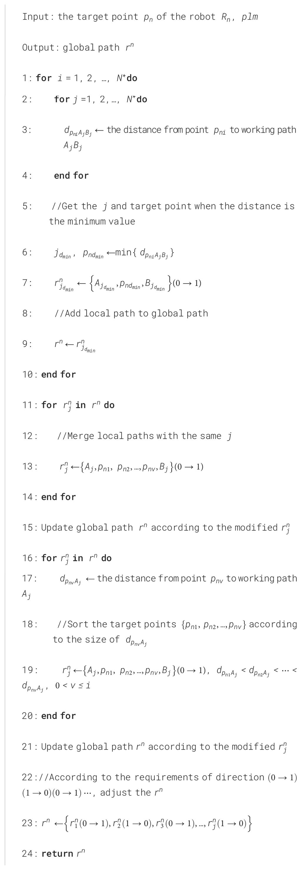
In order to get the serial number of working path and the robot’s moving direction, the geographic information is needed. Use straight lines and the endpoints and to generate a field map. Represent this map as a point-line map (). Use straight line as the baseline to generate other parallel line segment. As described in Algorithm 1, according to the straight-line equation of and the distance between each working path, the straight-line equations of all and the coordinates of the endpoints and are obtained. Finally, all working paths and endpoints and are stored in the .
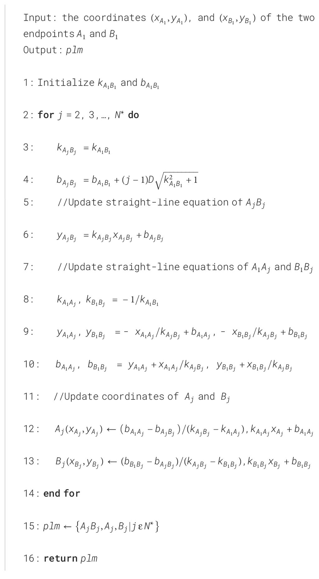
Algorithm 1. The plm generation method.
3.1.1 Calculating the equation of the working path
As shown in Figure 1, take as the baseline, and make parallel line segments , ,…,. Suppose the slope of line segment is , and the intercept is , then the straight-line equation of line segment is expressed as:
The coordinates , and of the two endpoints and of are obtained through the positioning device. Then the slope and intercept of are expressed as:
Since the straight line is parallel to the straight line , the slope of the straight line is equal to the slope of the straight line . According to the distance formula between two parallel lines, the intercept of the straight line is expressed as:
According to Equation 10, the straight-line equation of is expressed as:
The distance from straight-line segment to straight-line segment is 2 . Then according to Equation 10, the intercept of the straight line is expressed as:
According to Equation 12, the straight-line equation of is expressed as:
According to Equations 10-13, the straight-line equation of is expressed as:
According to the coordinates of the endpoints and , the straight-line equation of is obtained, and then the straight-line equations of all other working paths are obtained according to .
3.1.2 Calculating endpoint coordinates
According to the straight-line equation of obtained from Equation 14, determine the coordinates of the endpoints and . Make perpendicular lines and from point and point to line segment , and the foot points are and . Let the slopes of line segments and be and , and the intercepts be and , respectively. Then the straight-line equations of and are expressed as,
Substitute the coordinates of point into the straight-line equation of to obtain the intercept of , as shown in Equation 16.
The straight-line equation of can be obtained according to the intercept and slope . Then combine the linear equations of and to obtain the coordinates of the foot point as , as shown in Equations 17, 18.
The coordinate of the foot point is represented as,
Finally, according to Equations 14, 17-20 and the coordinates of the endpoints and , the coordinates and of all other endpoints can be obtained.
3.1.3 Fusion of endpoints and lines
The straight-line equation of and the coordinates of endpoints and are obtained from Sections 3.1.1 and 3.1.2, where the straight-line equation of includes information such as slope , intercept , and serial number . Use to represent endpoints , , and working path , as shown in Equation 21.
The provides detailed field information for the robot, supporting the robot to obtain its own direction, serial number of working paths, and path.
3.2 Robots global path generation method
When a robot detects a work conflict, it needs to re-plan the path for the low-priority robot. In order to quickly plan new paths, we first use and target points to generate the local path of each working path. Then, all local paths are merged into the global path of the robot, as shown in Algorithm 2. When the robot needs to adjust its path, it only needs to change the order and direction of the local path. Figure 3A shows all target points of the robot. Figure 3B shows global path and all local paths of the robot.
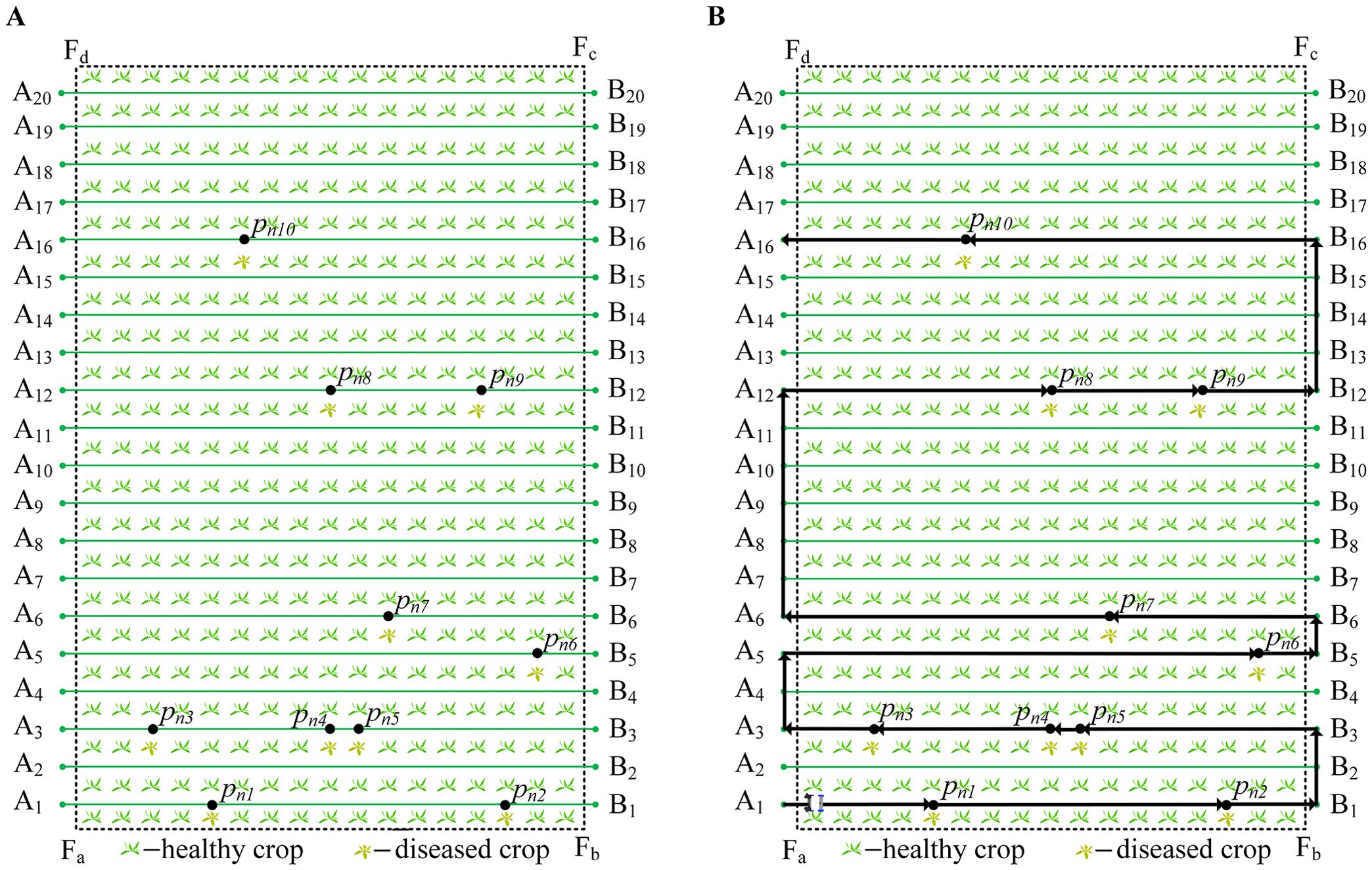
Figure 3. Target point and global path. (A) Target point. (B) Global path.
Algorithm 2. Robots global path generation method.
3.2.1 The local path of the robot
According to the and target point of the robot , plan the local path of the robot. Let the coordinates of be , and calculate the distance from point to straight line according to Equation 22.
Let represent the serial number of the working path when takes the minimum value, as shown in Equation 23. When takes the minimum value, the target point is in the working path
.
The endpoints and of the working path and point constitute the local path , as shown in Equation 24. Put between points and because the robot starts from the endpoint or and then passes through the target point
.
Calculate the distance from point to according to Equation 25 when two or more target points are in the same working path.
Sort the target points according to the size of , and then update the local path , as shown in Equation 26.
In Figure 3A, and are in the working path . Since , the path is obtained.
According to the target point , a series of local paths , , ,…, are obtained. For example, Figure 3A contains target points , and six groups of local paths are obtained, as shown in Equation 27.
3.2.2 Robots global path generation method
According to the local path of the robot, it is known that the serial number of the working path is . Sort the local paths according to and then get the path . For example, the path sorting in Figure 3A results in .
However, the sorted cannot be directly used as a robot’s global path because the connection between local paths is not continuous. For example, to in Equation 27 is from point to and finally to , which does not conform to the ‘U’ shape path of the robot. The robot cannot go directly from to but should go from to , then to . Therefore, it is necessary to adjust to , and at the same time, reorder the target points inside according to Equation 25 to obtain the updated . Similarly, update , , , according to this rule, and finally update the six groups of local paths in Equation 27 to get Equation 28.
Therefore, to ensure that the local paths are continuous, the direction between the local paths must satisfy or . satisfies Equation 29 or 30.
Combining the six groups of local paths in Equation 28, the global path is obtained, as shown in Equation 31. Finally, according to the target point of the robot in Figure 3A, plan the black path in Figure 3B.
3.3 Itinerary table with all global information
Based on the and its own position, the robot can calculate the direction of the robot, the number of the current working path, and the type of path. Combined with the global path and priority, the robot can learn all global information. When robot learns its own information, it needs to send its global information to other robots so that other robots can understand the status of , thereby judging the relationship between robots and predicting the possibility of collision. We designed an itinerary table (as shown in Table 1) that contains the robot’s serial number, priority, path type, moving direction, real-time position, target position, current serial number of the working path and last serial number of the working path to facilitate the robot’s sending and receive. When robot is started, it generates an itinerary table .` represents the itinerary table of a group of working robots, and represents the itinerary table of robot , as shown in Equation 32.
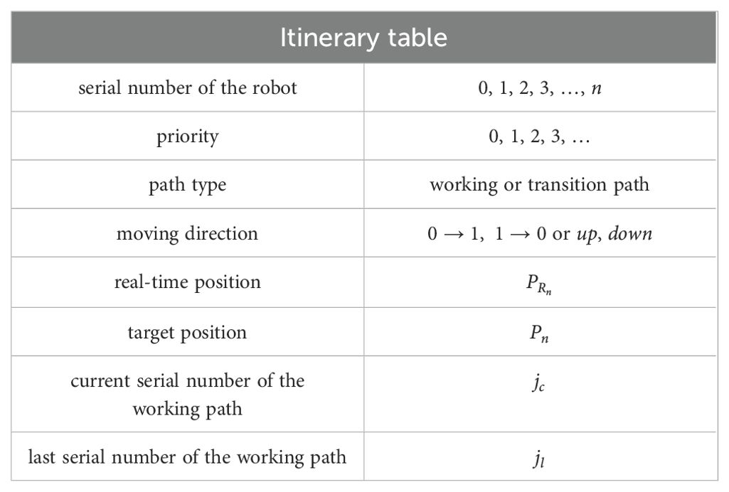
Table 1. The itinerary table of robot .
represents other itinerary tables except for , as shown in Equation 33.
Robot constantly updates the data in the itinerary table while working and broadcasts its to other robots . At the same time, robot receives and makes decisions.
3.4 Multi-robot collision avoidance method
Based on the point-line map, global path and itinerary table, the robot can understand the global information of the field and the status of other robots. With this information, the robot can make reasonable decisions and avoid collisions with other robots. The multi-robot collision avoidance algorithm is shown in Algorithm 3. We calculate the direction of the robot in different path type through Equations 5, 6. Then obtain the moving direction of other robots through the received itinerary table . Finally, we can compare whether the robots have the same direction.
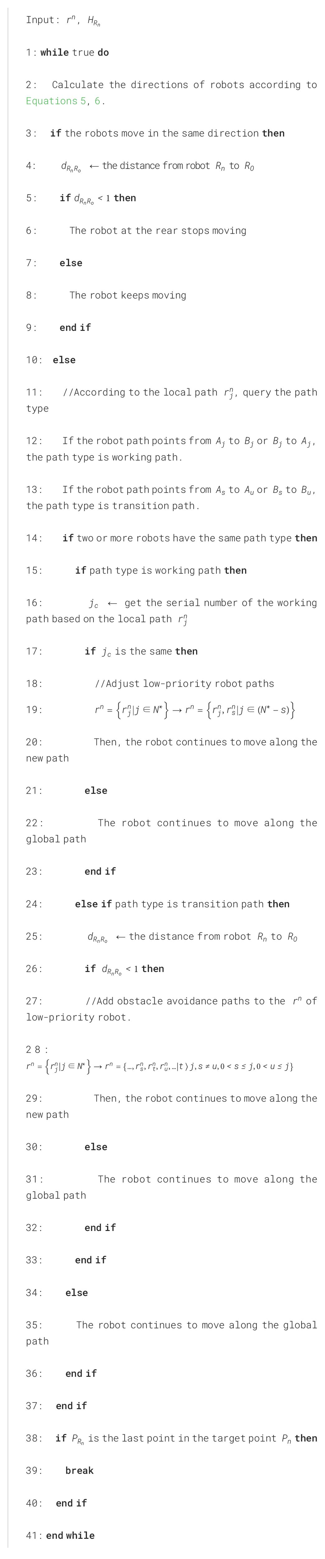
Algorithm 3. Multi-robot collision avoidance method.
If the direction is the same, query the real-time position of the robot with the same direction in the itinerary table , and calculate the distance between and . When , and maintain the current moving state. When , the robot at the rear stops moving, and when , the robot at the rear resumes moving.
But if the directions are different, the robot must make different decisions depending on the path type. We determine the path type of the robot based on its local path. If the robot path is from to or to , the path type of the robot is a working path. If the robot’s path is from to or to , the path type of the robot is a transition path.
3.4.1 On the working path
If the path types of multiple robots are working path, we query the current serial number of the working path of the robot through the local path .If the serial number is different, and are not in the same working path, and there is no possibility of conflict. Robots continue to move according to the global path and do not need to do anything.
If the serial number is the same, and are in the same working path, and conflicts or collisions will occur. There are two conflict cases: The first case is that one robot is moving in the working path, and another robot is moving from the transition path to the working path; The second is that all robots are entering the working path from the transition path.
For the first case, for example, when is already moving in the working path , is moving from to . Since they are going in different directions, they must collide. We do not consider the priorities of the robots at this time, directly let the robot give up the current working path, and then re-plan the global path. In order not to hinder the robot’s work and quickly generate the remaining path of the robot, we move the current conflicting local path to the end of the global path, as shown in Equation 34. Then, using the content of Section 3.2.2, according to the direction continuity between local paths, modify the target point order of the local path, and then update . The robot continues to move according to the updated .
For the second case, for example, both and are moving on the transition path and have not yet reached the working path. At this time, consider the priority of and , assuming that the priority of is lower than . The robot with low priority abandons the current working path and re-plans the path. The remaining path re-planning rules are the same as in the first case.
3.4.2 On the transition path
If multiple robots are on a transition path, we first query the real-time positions of the robots on the same path type. Then, calculate the distance between the robots. When , robots maintain the current moving state. When , the robot with low priority avoids the one with high priority. Since the width of the transition path is generally relatively wide, multiple robots can be accommodated simultaneously in the lateral direction. We can add some extra paths to avoid robot collisions.
In Figure 4A, robot goes from point to , robot goes from point to . It is obvious that and have different directions. R1 and R2 are close together and are about to collide. Assuming that robot has a lower priority than robot . The low-priority robot translates the current local path a certain distance to the left or right to avoid collision. For example, in Figure 4B, robot translates the local path to to avoid collision with . After translating the local path, the path is updated to {} according to the continuity of the path. We set the new path to , as shown in Equation 35.
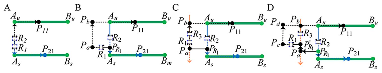
Figure 4. Conflict detection for robots on transition paths. (A) and meet at the transition path. (B) plans a new path. (C) meets on the new path. (D) plans a new path again.
The conflict occurs on the transition path , and is located between the local paths and , so insert between and , as shown in Equation 36. The moving direction of the robot on the transition path is or , and it is or on the working paths and , so insert between and , and the direction between other local paths in still satisfies or . Therefore, we only need to simply insert the local obstacle avoidance path between and without doing other operations.
When a new robot is detected, the low-priority robot continues to translate the local path left or right. In Figure 4C, robot is detected on path after passes through point , and robot plans local avoidance path , as shown in Equation 37.
Update according to the local avoidance path , as shown in Equation 38. Then insert the updated into the global path .
The updated local avoidance path is shown in Figure 4D. If conflicts with other robots again, plan the local obstacle avoidance path according to this rule and then update and .
4 Experiment and result
4.1 Simulate initial conditions
In order to verify our proposed multi-robot collision avoidance method, we used Gazebo software to design the robot working environment. The working environment includes field, crops, roads, and four working robots, as shown in Figure 5. Each working robot contains a medicine storage barrel, a medicine spraying device, communication device, positioning device and controller.
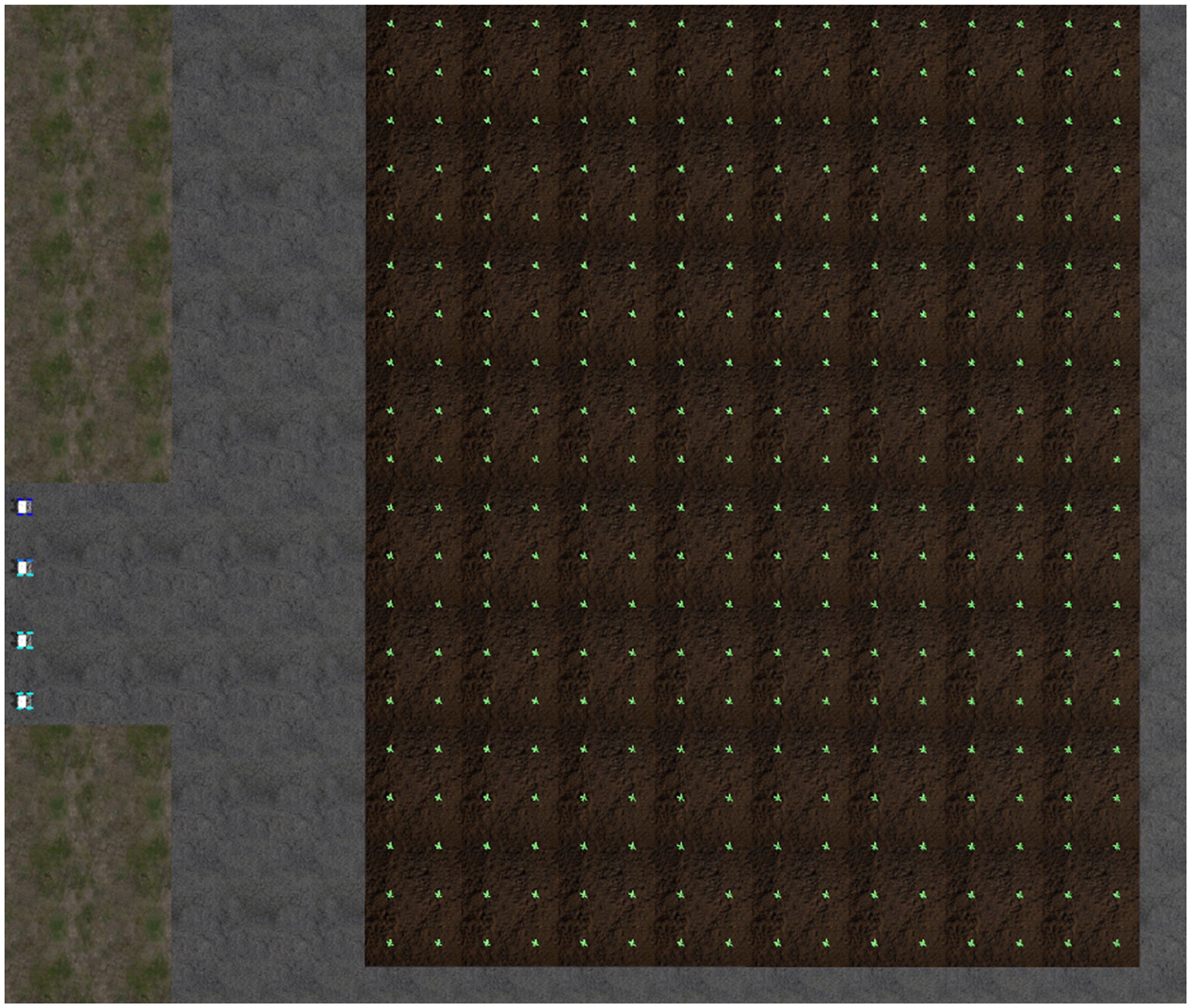
Figure 5. The robot’s simulation work environment.
In order to facilitate the description of the working process of the robot, a GUI display interface is designed to display the garage, field, crops, and robot, as shown in Figure 6. Set up a group of working robots , with priorities of 0, 1, 2, and 3, respectively. Set the field length to 20 meters and width to 16 meters. The field has 20 rows of crops (), and the distance between each row of crops is 1 meter (). The coordinate system is established with point as the origin, and the coordinates of the two endpoints and of the baseline are set to (0, -9) and (16, -9), respectively.
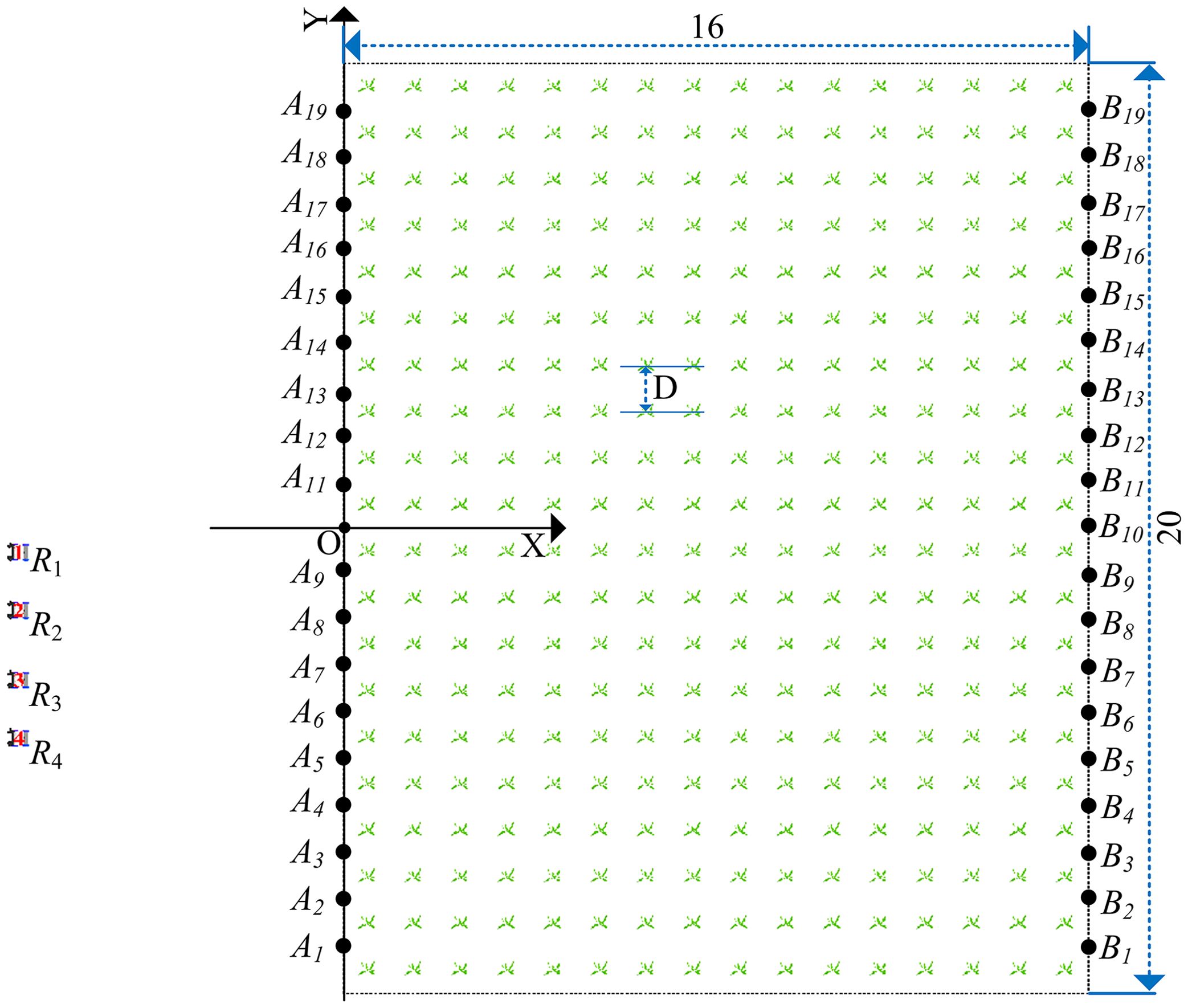
Figure 6. The initial diagram of the robot’s working environment.
4.2 Generating a point-line map
We first generate all working path and endpoints and based on the baseline . Calculate the slope and intercept of the working path based on points and and the straight-line equation of , as shown in Equation 39.
According to Equations 14, 39, calculate the straight-line equation of the working path , as shown in Equation 40.
Then according to Equations 17-20, the coordinates of points and are obtained as , (. Finally, according to Equations 39, 40, the is obtained as shown in Equation 41.
4.3 Generating the global path
We randomly generated the coordinates of 35 diseased crops, and then used them as the target points of the robot (Meshram et al., 2022). The target point is denoted as . Then, the coordinates are randomly assigned to , , , and , as shown in Figure 7. Randomly divide the targets into four groups: is represented by orange, is represented by black, is represented by blue, and is represented by purple.
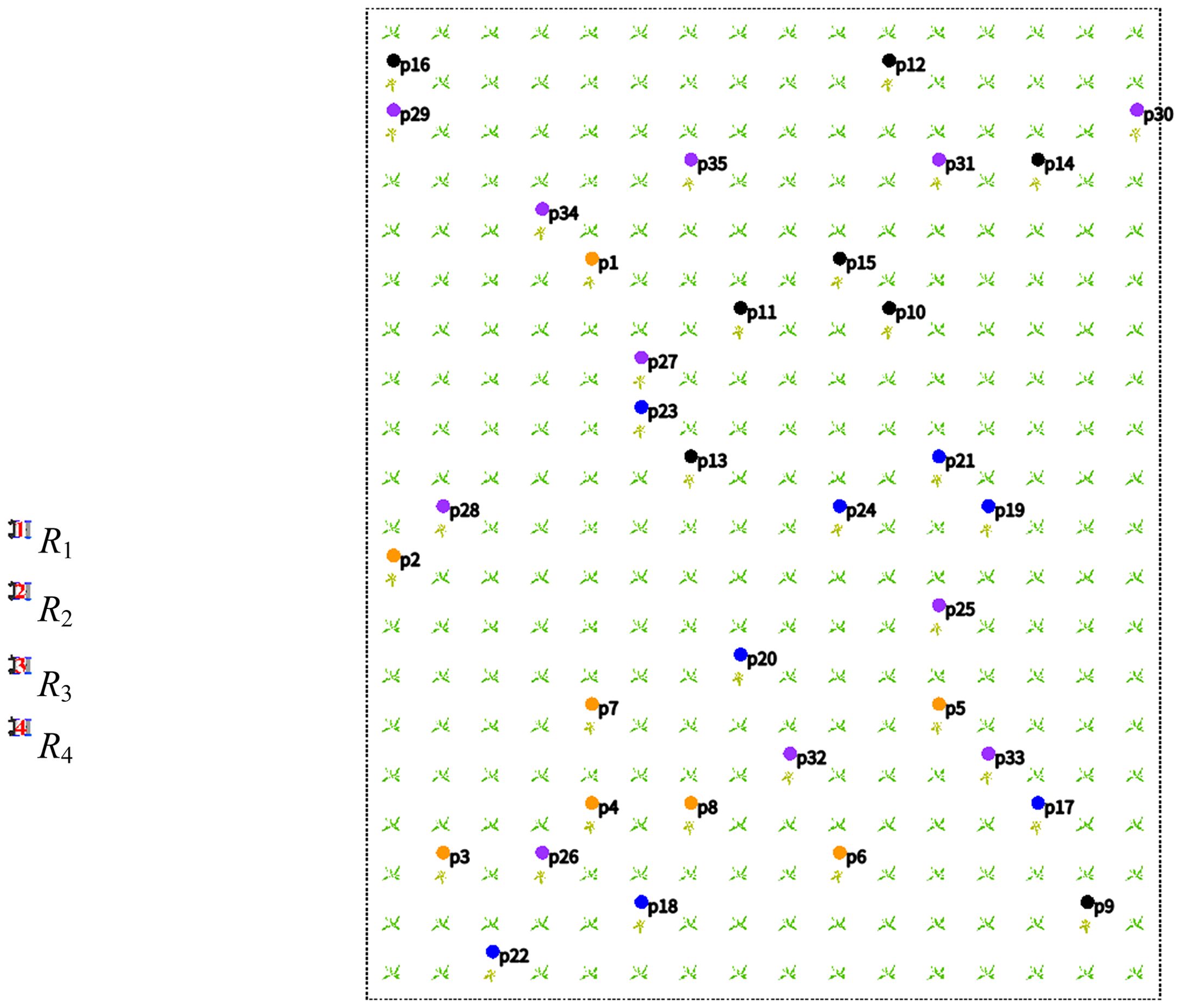
Figure 7. Random distribution of target points.
According to Section 3.2, use the target points and map to generate the robots’ global path, as shown in Equations 42-45.
where , , , , .
where , , , , , .
where , , , , , , .
where , , , , , , , .
Figures 8A–D show the global paths of , , , and .
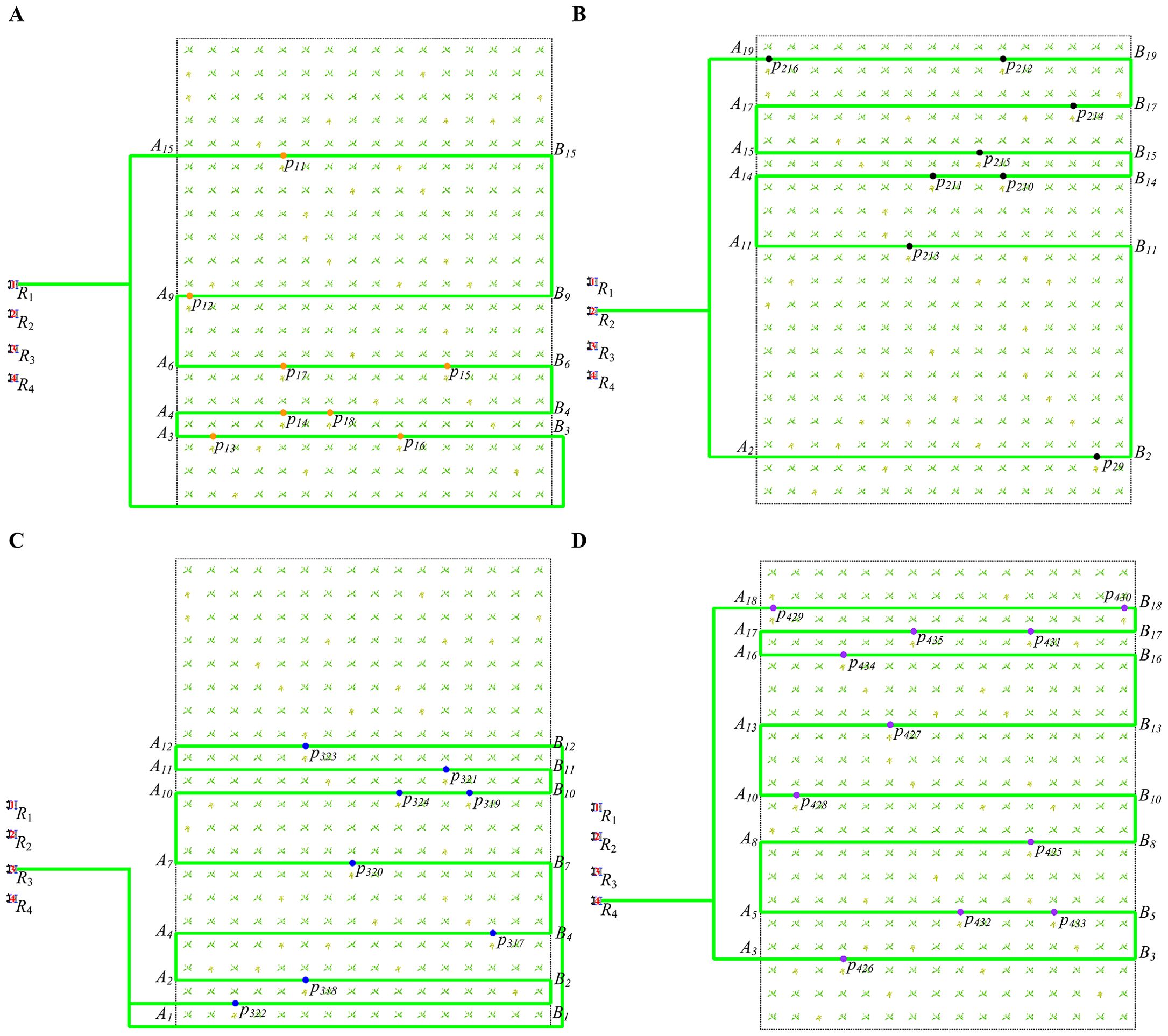
Figure 8. The global path of four robots. (A) The global path of . (B) The global path of . (C) The global path of . (D) The global path of .
4.4 Simulation experiment of multi-robot collision avoidance method
After planning the global path, the robots start spraying operations and simultaneously create an itinerary table , as shown in Table 1. During the operation, the robot determines the position, path, and direction of moving of other robots by querying their itinerary tables. Then, the robots detect four types of collision and conflict according to section 2.2. Next, the multi-robot collision avoidance method is simulated considering four types of collisions and conflicts.
4.4.1 Working path and different movement directions
When the serial number of the working path is the same, and the moving direction is different, there are two conflict cases: The first case is that one robot is moving in the working path, and another robot is moving from the transition path to the working path; The second is that all robots are entering the working path from the transition path.
Figure 9 shows the first case (The green path represents the path that has not been passed, while the black path represents the path that has already been passed). Robot is moving in the working path , and robot is moving from the transition path to the working path . Figure 9A shows that at 121 seconds, robot is about to leave its current working path and move to the next working path for work. Figure 9B shows that at 125s, robot moves to the transition path and detects a robot (At 25 seconds, works on working path , as shown in Figure 9C) with a different direction of moving in the working path according to the itinerary table.
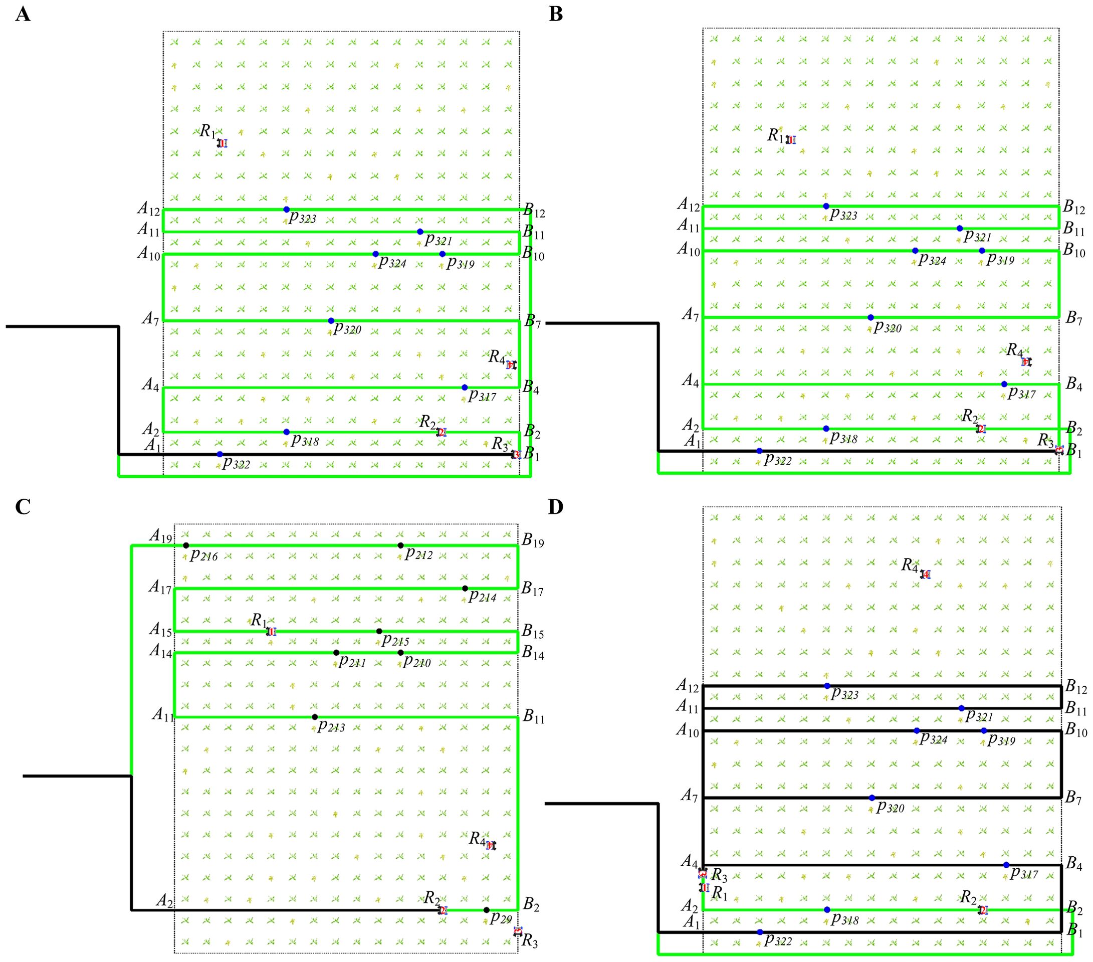
Figure 9. The paths of robots moving in different directions on the same working path at different times (the first case). (A) The path of robot at 121 seconds. (B) The path of robot at 125 seconds. (C) The path of robot at 125 seconds. (D) The path of robot at 522 seconds.
In order to avoid collision, robot will abandon the current local path and then re-plan the remaining path. We follow the method proposed in Section 3 and first move the current local path to the end of the global path , as shown in Equation 46. But in the global path , and do not satisfy the continuity of direction, and () to () appear, so we need to change the direction of the remaining path , , , , and .
where , , , , , ,
We change the direction of the local path by modifying the order of the points of the local path, as shown in Equation 47. The robot continues driving along the updated path . Figure 9D shows that at 522 seconds, robot moves to the last working path, and the black path in the figure clearly shows the updated new path.
where , , , , , , .
Figure 10 shows the second case. Robots and move to the same working path from other paths. Figure 10A shows that at 10 seconds, robot is about to leave its current working path and move to the next working path . Figure 10B shows that at 13 seconds, robot reaches the transition path and begins to move toward the working path . At this time, it is detected that another robot (Figure 10C shows the operational status of at 13 seconds) is also moving toward the working path according to the itinerary table.
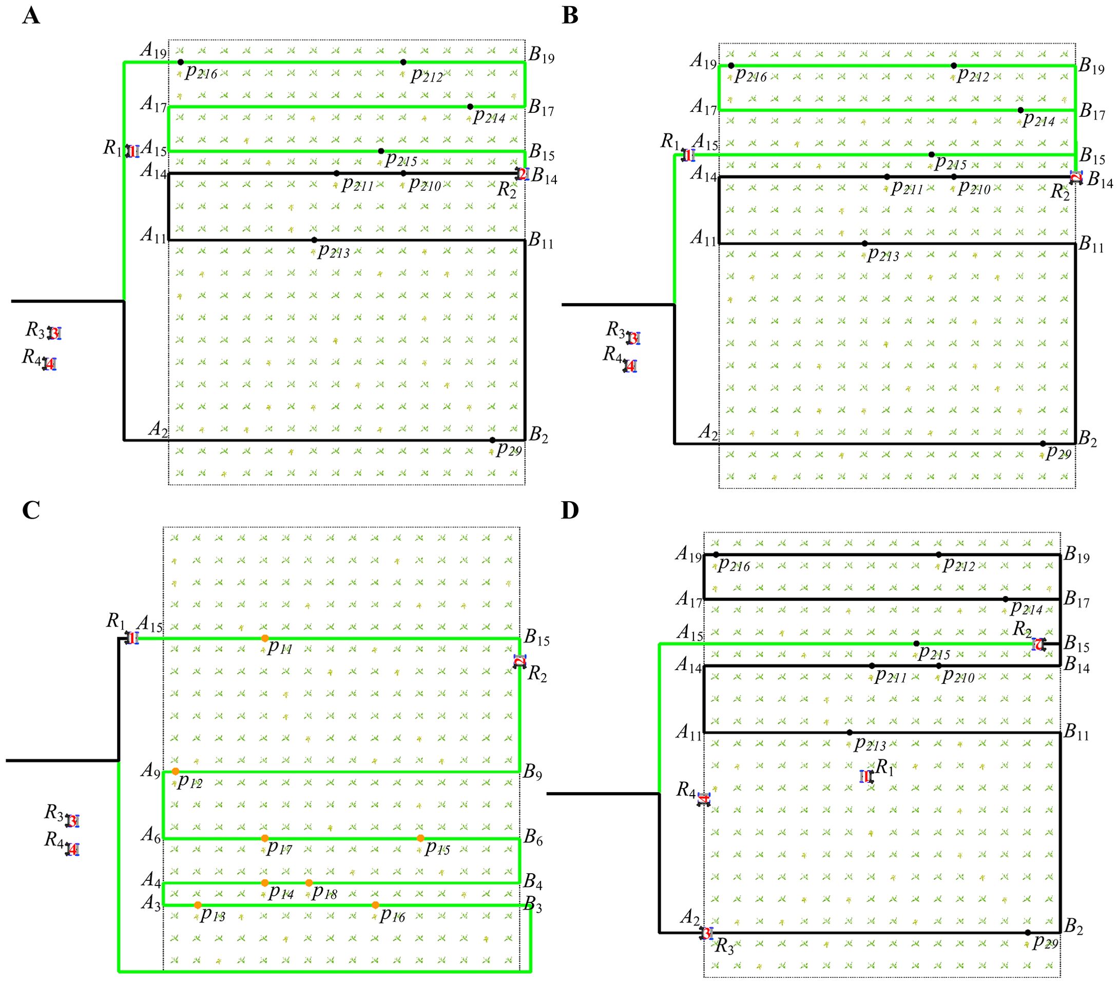
Figure 10. The paths of robots moving in different directions on the same working path at different times (the second case). (A) The path of robot at 10 seconds. (B) The path of robot at 13 seconds. (C) The path of robot at 13 seconds. (D) The path of robot at 173 seconds.
Since has a higher priority than , in order to avoid collision, abandons the current local path and re-plans a new path. The global path update method of is the same as Equations 46, 47. The updated path of is as shown in Equation 48. Figure 10D shows that at 173 seconds, the robot moves to the last working path, and the black path in the figure clearly shows the updated new path.
where , , , , , .
4.4.2 Working path and same movement direction
When the robots have the same serial number and the same moving direction, there are two cases: The robots maintain the current speed and move in the order of one after the other. The second is that when one of the robots stops working at the target point, the other robots at the back must wait for the front robot to complete the work.
Figure 11 shows the first case. Robots and maintain a certain speed and distance, and move in a front-to-back sequence. Figure 11A shows the states of robots and at 11 seconds. Figure 11B shows that at 31 seconds, robot and keep moving forward in this state.
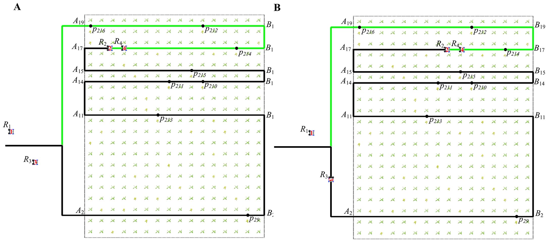
Figure 11. The paths of robots moving in the same direction on the same working path at different times (the first case). (A) The path of robot at 11 seconds. (B) The path of robot at 31 seconds.
Figure 12 shows the second case. Robot stops moving and performs the spraying operation after reaching the target point . Robot stops moving, waiting for robot to complete the operation. Figure 12A shows that at 33 seconds, robot moves toward along the path. As depicted in Figure 12B, robot detects the halt of at 36 seconds, and maintains a safe distance from when it stops. Figure 12C shows that at 36 seconds, robot fpls.2024.1393541 stops at the target point . Figure 12D shows that at 39 seconds, robot stops moving until completes the work.
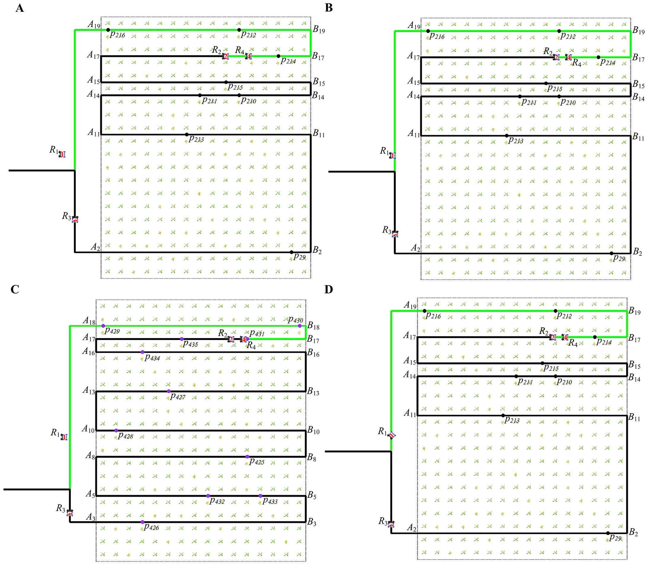
Figure 12. The paths of robots moving in the same direction on the same working path at different times (the second case). (A) The path of robot at 33 seconds. (B) The path of robot at 36 seconds. (C) The path of robot at 36 seconds. (D) The path of robot at 39 seconds.
4.4.3 Transition path and same movement direction
When the robot is on the transition path and moves in the same direction as other robots, there are two cases: One is that the robot keeps the current speed and follows the others. The other is that when one of the robots turns to the working path, the robots behind stop at a safe distance and wait for the turn to finish.
The first case is the same as the first case in 4.4.2. As long as the safe distance between robots is ensured, no other operations are performed.
Figure 13 shows the second case, robots and are moving on the transition path. Figure 13A shows that at 11 seconds, robot detects that is moving from the working path to the transition path , and stops moving and waits for to complete the turn. Figure 13B shows that at 15 seconds, after completes its turn, and maintain a certain safe distance and move along the transition path . Figure 13C shows that at 22 seconds, robot maintains a safe distance from and moves in the same direction. Figure 13D shows that at 30 seconds, robot switches from the transition path to the working path , and robot stops at a safe distance, waiting for robot to finish the turn.
Figure 13. The paths of robots moving in the same direction on different working paths at different times. (A) The path of robot at 11 seconds. (B) The path of robot at 15 seconds. (C) The path of robot at 22 seconds. (D) The path of robot at 30 seconds.
4.4.4 Transition path and different movement directions
Figure 14 shows that robots , , and are moving on the transition path. The and of are 4 and 6 respectively. The and of are 11 and 2 respectively. The and of are 4 and 6 respectively. According to Equation 6, their directions on the transition path are down, up, and down respectively. The moving direction of is different from that of and . Change the priority of , , and to 0, 2, and 1, respectively.
Figure 14. The paths of robots moving in different directions on different working paths at different times. (A) The path of robot at 31 seconds. (B) The path of robot at 31 seconds. (C) The path of robot at 47 seconds. (D) The path of robot at 47 seconds. (E) The path of robot at 56 seconds.
Figure 14A shows that at 31 seconds, robot detects that (Figure 14B shows the global path of at 31 seconds) is approaching from the opposite direction. Since the priority of is lower than that of , plans the obstacle avoidance path according to Section 3.4.2. translates the current local path a certain distance to the right and adds a new obstacle avoidance path , as shown in Equation 49.
Then, we directly insert between and in , as shown in Equation 50. moves according to updated . Figure 14C shows the new path of .
where , , , , , , .
detects a new robot (Figure 14D shows the global path of at 47 seconds) approaching from the opposite direction at 47 seconds in Figure 14C. Since has a lower priority than , plans an obstacle avoidance path to avoid colliding with . Just like the rules for avoiding , move the current local path a certain distance to the right, and then update the local path , as shown in Equation 51.
Then, we directly insert the updated between and in , as shown in Equation 52. moves according to updated . Figure 14E shows the new path of at 56 seconds.
where .
4.5 Analysis of experimental results
4.5.1 Analysis of multi-robot collision avoidance results
We recorded the number of times the multi-robot system avoided collisions and the time spent executing tasks for various numbers of target points, as shown in Table 2. We randomly generated sets of 15, 25, 35, and 45 target points and conducted 10 experiments for each set, with target points randomly generated in each experiment. For the multi-robot system, we recorded the total number of collisions avoided and the total time spent on task execution for each robot. For a single robot, we recorded only the total time spent on the spraying task.
Table 2. Experimental results (The total number of collisions avoided and the total time spent on the task for each robot).
As shown in Table 2, under different numbers of target points, the time taken by the multi-robot system to complete the task is much shorter than that of a single robot. Specifically, for 15 target points, the multi-robot system avoids collisions 119 times in total, saving 55.6% of the time compared to a single robot. For 25 target points, the multi-robot system avoids collisions 130 times in total, saving 57.9% of the time compared to a single robot. For 35 target points, the multi-robot system avoids collisions 140 times in total, saving 48.9% of the time compared to a single robot. For 45 target points, the multi-robot system avoids collisions 145 times in total, saving 40.7% of the time compared to a single robot. The experimental results show that under the same number of target points, the multi-robot system can complete the spraying task while avoiding collisions or conflicts between robots, and the completion time can be reduced by more than 40%.
4.5.2 Comparison experiment with other methods
To evaluate our method, we compare it with the classic Reciprocal Velocity Obstacles (RVO) (Van den Berg et al., 2008) and Optimal Reciprocal Collision Avoidance (ORCA) (Niu et al., 2021) algorithms. In terms of time complexity, the time complexity of RVO and ORCA algorithms is O(n2). As shown in Algorithms 1–3, their time complexity are O(n), O(n2), and O(n), respectively. Therefore, the overall time complexity of our algorithm is O(n2).
Since the width of the working path in the field is relatively narrow, it cannot support two robots moving side by side. When two robots move toward each other on the working path (as shown in Figure 2B), if the low-priority robot performs an evasive action, it will inevitably collide with the crops. Therefore, we made some modifications to the RVO and ORCA algorithms. If they are detected to be moving in opposite directions on the working path, the low-priority robot stops and waits for the other robot to complete the work before continuing the work. Under the same settings, ten spraying tests with the same number and the same order are conducted for each collision avoidance method with different numbers of target points. The completion time mainly reflects the efficiency of different methods, and the number of collisions avoided reflects the performance from the side.
The experimental results are shown in Table 3, demonstrating that the proposed collision avoidance algorithm outperforms the RVO and ORCA algorithms. Specifically, for 15 target points, the completion time of our algorithm is reduced by 5.2% and 2.9% compared with RVO and ORCA, respectively. This is because when the number of target points is relatively small, the probability of collision or conflict between robots in a large field is relatively small, so the total completion time is not much different. For 25 target points, the completion time is reduced by 9.8% and 3.8% compared with the RVO and ORCA algorithms, respectively. For 35 target points, the completion time is reduced by 14.9% and 8.2% compared with the RVO and ORCA algorithms, respectively. For 45 target points, the completion time is reduced by 16.8% and 9.5% compared with the RVO and ORCA algorithms, respectively. As the number of target points increases, the likelihood of collisions or conflicts between robots also increases. Our proposed algorithm demonstrates better performance, with a greater reduction in completion time compared to RVO and ORCA. In addition, the number of collision avoidance of our proposed algorithm is less than that of RVO and ORCA. This is because our collision avoidance algorithm can pre-judge potential collisions or conflicts on the working path, thereby reducing their occurrence. In summary, our proposed algorithm can complete the spraying task on large-scale fields in a timely and efficient manner, exhibiting high operational efficiency.
Table 3. Experimental results of different collision avoidance methods.
4.6 Summary
We designed a simulation environment for precise spraying of sweet potato fields, and then experimentally verified the collision avoidance method we proposed against four types of collisions or conflicts that may occur between multiple robots in the field. We demonstrate that our multi-robot collision avoidance method can be well deployed on robots even though they only have communication modules, positioning modules and low-cost control chips. We validate the collision avoidance strategy in various collision or conflict scenarios and show that our method can run robustly for long periods of time without collisions.
5 Conclusion
In this article, we propose a multi-robot collision avoidance method that only uses point-line maps and real-time robot positions to determine the relationship between robots, make reasonable decisions, and avoid collisions between robots. We evaluate the performance of our method through a series of comprehensive experiments and demonstrate that the collision avoidance method is simple and efficient in terms of success rate, safety, and navigation efficiency. For the current situation where only a single robot is used to complete the operation, the method we proposed can greatly improve the efficiency of farmland robot operations. At the same time, the method we proposed has extremely low requirements for robot hardware performance, which greatly reduces the cost of each robot, thereby reducing farmers’ farmland management costs and labor intensity, and indirectly increasing farmers’ economic income. It provides the theoretical basis and technical support for reducing the cost of multi-robot systems and accelerating the promotion and application of multi-robot systems in agriculture.
Our work is a first step toward reducing robot costs, avoiding robot collisions, and improving the efficiency of multi-agricultural robots. Although we are fully aware that as a local collision avoidance method, our approach cannot completely replace reinforcement learning-based multi-robot path planners when scheduling. Our future work will be how to extend our method to larger-scale robot systems at low cost and apply this method to real field environments to achieve a safe and efficient multi-robot collision avoidance method.
Data availability statement
The original contributions presented in the study are included in the article/supplementary material. Further inquiries can be directed to the corresponding author.
Author contributions
KX: Writing – original draft, Writing – review & editing. JX: Supervision, Validation, Writing – review & editing. WS: Conceptualization, Investigation, Writing – review & editing. PX: Data curation, Methodology, Writing – review & editing. RY: Methodology, Supervision, Writing – review & editing.
Funding
The author(s) declare financial support was received for the research, authorship, and/or publication of this article. This research was funded by the Key R&D Projects in Hainan Province (Grant No. ZDYF2023XDNY039) and National Talent Foundation Project of China (Grant No. T2019136).
Acknowledgments
The authors would like to thank their schools and colleges, as well as the funding of the project. All support and assistance are sincerely appreciated. Additionally, we sincerely appreciate the work of the editor and the reviewers of the present paper.
Conflict of interest
The authors declare that the research was conducted in the absence of any commercial or financial relationships that could be construed as a potential conflict of interest.
Publisher’s note
All claims expressed in this article are solely those of the authors and do not necessarily represent those of their affiliated organizations, or those of the publisher, the editors and the reviewers. Any product that may be evaluated in this article, or claim that may be made by its manufacturer, is not guaranteed or endorsed by the publisher.
References
Alonso-Mora, J., Breitenmoser, A., Rufli, M., Beardsley, P., Siegwart, R. (2013). “Optimal reciprocal collision avoidance for multiple non-holonomic robots,” in Distributed autonomous robotic systems: The 10th international symposium (Berlin, Germany: Springer Berlin Heidelberg), 203–216.
Althoff, D., Kuffner, J. J., Wollherr, D., Buss, M. (2012). Safety assessment of robot trajectories for navigation in uncertain and dynamic environments. Autonomous Robots 32, 285–302. doi: 10.1007/s10514-011-9257-9
Baltazar, A. R., Santos, F. N. D., Moreira, A. P., Valente, A., Cunha, J. B. (2021). Smarter robotic sprayer system for precision agriculture. Electronics 10, 2061. doi: 10.3390/electronics10172061
Cai, C., Yang, C., Zhu, Q., Liang, Y. (2007). “Collision avoidance in multi-robot systems,” in 2007 International Conference on Mechatronics and Automation. 2795–2800 (Harbin, China: IEEE).
Carbone, C., Garibaldi, O., Kurt, Z. (2018). Swarm robotics as a solution to crops inspection for precision agriculture. KnE Eng. 3, 552–562. doi: 10.18502/keg.v3i1.1459
Chang, L., Shan, L., Jiang, C., Dai, Y. (2021). Reinforcement based mobile robot path planning with improved dynamic window approach in unknown environment. Autonomous robots 45, 51–76. doi: 10.1007/s10514-020-09947-4
Chen, Y. F., Everett, M., Liu, M., How, J. P. (2017a). “Socially aware motion planning with deep reinforcement learning,” in 2017 IEEE/RSJ International Conference on Intelligent Robots and Systems (IROS). (Vancouver, BC, Canada: IEEE), 1343–1350. doi: 10.1109/IROS.2017.8202312
Chen, Y. F., Liu, M., Everett, M., How, J. P. (2017b). “Decentralized non-communicating multiagent collision avoidance with deep reinforcement learning,” in 2017 IEEE international conference on robotics and automation (ICRA). (Singapore: IEEE), 285–292. doi: 10.1109/ICRA.2017.7989037
Cheng, P. D. C., Indri, M., Possieri, C., Sassano, M., Sibona, F. (2023). Path planning in formation and collision avoidance for multi-agent systems. Nonlinear Analysis: Hybrid Syst. 47, 101293. doi: 10.1016/j.nahs.2022.101293
Claes, D., Hennes, D., Tuyls, K., Meeussen, W. (2012). “Collision avoidance under bounded localization uncertainty,” in 2012 IEEE/RSJ International Conference on Intelligent Robots and Systems. (Vilamoura-Algarve, Portugal: IEEE), 1192–1198. doi: 10.1109/IROS.2012.6386125
Claes, D., Tuyls, K. (2018). Multi robot collision avoidance in a shared workspace. Autonomous Robots 42, 1749–1770. doi: 10.1007/s10514-018-9726-5
Danton, A., Roux, J. C., Dance, B., Cariou, C., Lenain, R. (2020). “Development of a spraying robot for precision agriculture: An edge following approach,” in 2020 IEEE Conference on Control Technology and Applications (CCTA). (Montreal, QC, Canada: IEEE), 267–272. doi: 10.1109/CCTA41146.2020.9206304
Fiorini, P., Shiller, Z. (1998). Motion planning in dynamic environments using velocity obstacles. Int. J. robotics Res. 17, 760–772. doi: 10.1177/027836499801700706
Godoy, J., Karamouzas, I., Guy, S., Gini, M. (2016). “Implicit coordination in crowded multi-agent navigation,” in Proceedings of the AAAI Conference on Artificial Intelligence, Vol. 30 (1). (Phoenix, Arizona, USA: AAAI Press). doi: 10.1609/aaai.v30i1.10131
Hameed, I. A., Bochtis, D., Sørensen, C. A. (2013). An optimized field coverage planning approach for navigation of agricultural robots in fields involving obstacle areas. Int. J. advanced robotic Syst. 10, 231. doi: 10.5772/56248
Han, Y., Zhan, I. H., Zhao, W., Pan, J., Zhang, Z., Wang, Y., et al. (2022). Deep reinforcement learning for robot collision avoidance with self-state-attention and sensor fusion. IEEE Robotics Automation Lett. 7, 6886–6893. doi: 10.1109/LRA.2022.3178791
He, H., Kamburugamuve, S., Fox, G. C., Zhao, W. (2016). Cloud based real-time multi-robot collision avoidance for swarm robotics. Int. J. Grid Distributed Computing 9, 339–358. doi: 10.14257/ijgdc
Hennes, D., Claes, D., Meeussen, W., Tuyls, K. (2012). “Multi-robot collision avoidance with localization uncertainty,” in Proceedings of the 11th International Conference on Autonomous Agents and Multiagent Systems-Volume 1. (Valencia, Spain: International Foundation for Autonomous Agents and Multiagent Systems), 147–154. doi: 10.5555/2343576.2343597
Hu, K., Chen, Z., Kang, H., Tang, Y. (2024). 3D vision technologies for a self-developed structural external crack damage recognition robot. Automation Construction 159, 105262. doi: 10.1016/j.autcon.2023.105262
Huang, S., Zhang, H., Huang, Z. (2022). Multi-UAV collision avoidance using multi-agent reinforcement learning with counterfactual credit assignment. arXiv preprint arXiv:2204.08594. doi: 10.48550/arXiv.2204.08594
Jawhar, I., Mohamed, N., Wu, J., Al-Jaroodi, J. (2018). Networking of multi-robot systems: Architectures and requirements. J. Sensor Actuator Networks 7, 52. doi: 10.3390/jsan7040052
Keshmiri, S., Payandeh, S. (2009). “A centralized framework to multi-robots formation control: Theory and application,” in International Workshop on Collaborative Agents, Research and Development (Springer Berlin Heidelberg, Berlin, Heidelberg), 85–98.
Kim, J., Son, H. I. (2020). A voronoi diagram-based workspace partition for weak cooperation of multi-robot system in orchard. IEEE Access 8, 20676–20686. doi: 10.1109/Access.6287639
Liu, L., Liu, Y., He, X., Liu, W. (2022). Precision variable-rate spraying robot by using single 3D LIDAR in orchards. Agronomy 12, 2509. doi: 10.3390/agronomy12102509
Long, P., Liu, W., Pan, J. (2017). Deep-learned collision avoidance policy for distributed multiagent navigation. IEEE Robotics Automation Lett. 2, 656–663. doi: 10.1109/LRA.2017.2651371
Matoui, F., Boussaid, B., Metoui, B., Abdelkrim, M. N. (2020). Contribution to the path planning of a multi-robot system: centralized architecture. Intelligent Service Robotics 13, 147–158. doi: 10.1007/s11370-019-00302-w
Meshram, A. T., Vanalkar, A. V., Kalambe, K. B., Badar, A. M. (2022). Pesticide spraying robot for precision agriculture: A categorical literature review and future trends. J. Field Robotics 39, 153–171. doi: 10.1002/rob.22043
Niu, H., Ma, C., Han, P. (2021). Directional optimal reciprocal collision avoidance. Robotics Autonomous Syst. 136, 103705. doi: 10.1016/j.robot.2020.103705
Oberti, R., Schmilovitch, Z. E. (2021). “Robotic spraying for precision crop protection,” in Innovation in agricultural robotics for precision agriculture: A roadmap for integrating robots in precision agriculture. (Springer, Cham), 117–150. doi: 10.1007/978-3-030-77036-5_6
Parker, L. E., Rus, D., Sukhatme, G. S. (2016). Multiple Mobile Robot Systems. In: Siciliano, B., Khatib, O. (eds) Springer Handbook of Robotics. (Springer, Cham: Springer Handbooks), 1335–1384. doi: 10.1007/978-3-319-32552-1_53
Pfeiffer, M., Schaeuble, M., Nieto, J., Siegwart, R., Cadena, C. (2017). “From perception to decision: A data-driven approach to end-to-end motion planning for autonomous ground robots,” in 2017 ieee international conference on robotics and automation (icra). (Singapore: IEEE), 1527–1533. doi: 10.1109/ICRA.2017.7989182
Raibail, M., Rahman, A. H. A., AL-Anizy, G. J., Nasrudin, M. F., Nadzir, M. S. M., Noraini, N. M. R., et al. (2022). Decentralized multi-robot collision avoidance: A systematic review from 2015 to 2021. Symmetry 14, 610. doi: 10.3390/sym14030610
Schwartz, J. T., Sharir, M. (1983). On the piano movers' problem: III. Coordinating the motion of several independent bodies: The special case of circular bodies moving amidst polygonal barriers. Int. J. Robotics Res. 2, 46–75. doi: 10.1177/027836498300200304
Snape, J., Van Den Berg, J., Guy, S. J., Manocha, D. (2009). “Independent navigation of multiple mobile robots with hybrid reciprocal velocity obstacles,” in 2009 IEEE/RSJ International Conference on Intelligent Robots and Systems. (St. Louis, MO, USA: IEEE), 5917–5922. doi: 10.1109/IROS.2009.5354821
Sun, D., Kleiner, A., Nebel, B. (2014). “Behavior-based multi-robot collision avoidance,” in 2014 IEEE international conference on robotics and automation (ICRA). (Hong Kong, China: IEEE), 1668–1673. doi: 10.1109/ICRA.2014.6907075
Tang, Y., Qi, S., Zhu, L., Zhuo, X., Zhang, Y., Meng, F. (2024). Obstacle avoidance motion in mobile robotics. J. System Simulation 36, 1–26. doi: 10.16182/j.issn1004731x.joss.23-1297E
Tang, S., Thomas, J., Kumar, V. (2018). Hold or take optimal plan (hoop): A quadratic programming approach to multi-robot trajectory generation. Int. J. Robotics Res. 37, 1062–1084. doi: 10.1177/0278364917741532
Ünal, İ., Kabaş, Ö., Eceoğlu, O., Moiceanu, G. (2023). Adaptive multi-robot communication system and collision avoidance algorithm for precision agriculture. Appl. Sci. 13, 8602. doi: 10.3390/app13158602
Van den Berg, J., Lin, M., Manocha, D. (2008). “Reciprocal velocity obstacles for real-time multi-agent navigation,” in 2008 IEEE international conference on robotics and automation. (Pasadena, CA, USA: IEEE), 1928–1935. doi: 10.1109/ROBOT.2008.4543489
Wang, D., Fan, T., Han, T., Pan, J. (2020). A two-stage reinforcement learning approach for multi-UAV collision avoidance under imperfect sensing. IEEE Robotics Automation Lett. 5, 3098–3105. doi: 10.1109/LSP.2016.
Xiao, W., Yuan, L., He, L., Ran, T., Zhang, J., Cui, J. (2022). Multigoal visual navigation with collision avoidance via deep reinforcement learning. IEEE Trans. Instrumentation Measurement 71, 1–9. doi: 10.1109/TIM.2022.3158384
Xiongkui, H. (2020). Research progress and developmental recommendations on precision spraying technology and equipment in China. Smart Agric. 2, 133. doi: 10.12133/j.smartag.2020.2.1.201907-SA002
Yu, J., LaValle, S. M. (2016). Optimal multirobot path planning on graphs: Complete algorithms and effective heuristics. IEEE Trans. Robotics 32, 1163–1177. doi: 10.1109/TRO.2016.2593448
Zhang, D., Chen, C., Zhang, G. (2024). “AGV path planning based on improved A-star algorithm,” in 2024 IEEE 7th Advanced Information Technology, Electronic and Automation Control Conference (IAEAC). (Chongqing, China: IEEE), Vol. 7, 1590–1595. doi: 10.1109/IAEAC59436.2024.10503919
Zhao, W., Wang, Y., Zhang, Z., Wang, H. (2021). Multicriteria ship route planning method based on improved particle swarm optimization–genetic algorithm. J. Mar. Sci. Eng. 9, 357. doi: 10.3390/jmse9040357
Keywords: multi-robot, accurate spraying, collision avoidance, sweet potatoes, itinerary table
Citation: Xu K, Xing J, Sun W, Xu P and Yang R (2024) Multi-robot collision avoidance method in sweet potato fields. Front. Plant Sci. 15:1393541. doi: 10.3389/fpls.2024.1393541
Received: 29 February 2024; Accepted: 16 August 2024;
Published: 10 September 2024.
Edited by:
Daobilige Su, China Agricultural University, ChinaReviewed by:
Xiangjun Zou, South China Agricultural University, ChinaJános Botzheim, Eötvös Loránd University, Hungary
Copyright © 2024 Xu, Xing, Sun, Xu and Yang. This is an open-access article distributed under the terms of the Creative Commons Attribution License (CC BY). The use, distribution or reproduction in other forums is permitted, provided the original author(s) and the copyright owner(s) are credited and that the original publication in this journal is cited, in accordance with accepted academic practice. No use, distribution or reproduction is permitted which does not comply with these terms.
*Correspondence: Ranbing Yang, eWFuZ3JhbmJpbmdAMTYzLmNvbQ==