Research on methods for estimating reference crop evapotranspiration under incomplete meteorological indicators

Background: Accurate estimation of reference crop evapotranspiration (ET₀) is crucial for farmland hydrology, crop water requirements, and precision irrigation decisions. The Penman-Monteith (PM) model has high accuracy in estimating ET₀, but it requires many uncommon meteorological data inputs. Therefore, an ideal method is needed that minimizes the number of input data variables without compromising estimation accuracy. This study aims to analyze the performance of various methods for estimating ET₀ in the absence of some meteorological indicators. The Penman-Monteith (PM) model, known for its high accuracy in ET₀ estimation, served as the standard value under conditions of adequate meteorological indicators. Comparative analyses were conducted for the Priestley-Taylor (PT), Hargreaves (H-A), McCloud (M-C), and FAO-24 Radiation (F-R) models. The Bayesian estimation method was used to improve the ET estimation model.

Results: Results indicate that, compared to the PM model, the F-R model performed best with inadequate meteorological indicators. It demonstrates higher average correlation coefficients (R²) at daily, monthly, and 10-day scales: 0.841, 0.937, and 0.914, respectively. The corresponding root mean square errors (RMSE) are 1.745, 1.329, and 1.423, and mean absolute errors (MAE) are 1.340, 1.159, and 1.196, with Willmott's Index (WI) values of 0.843, 0.862, and 0.859. Following Bayesian correction, R² values remained unchanged, but significant reductions in RMSE were observed, with average reductions of 15.81%, 29.51%, and 24.66% at daily, monthly, and 10-day scales, respectively. Likewise, MAE decreased significantly, with average reductions of 19.04%, 34.47%, and 28.52%, respectively, and WI showed improvement, with average increases of 5.49%, 8.48%, and 10.78%, respectively.

Conclusion: Therefore, the F-R model, enhanced by the Bayesian estimation method, significantly enhances the estimation accuracy of ET₀ in the absence of some meteorological indicators.

1 Introduction

Agriculture stands as the largest consumer of freshwater (Food, and Nations, A. O. o. t. U, 2017; Boretti and Rosa, 2019). Efficient freshwater resource utilization in agricultural product production is a pivotal concern for sustainable development (Tunalı et al., 2023). Particularly in arid or semiarid climates, irrigation plays a critical role in food production systems and economies. However, limited available water may not meet the demands of food production, necessitating effective scheduling methods to optimize crop yields with constrained water resources (King et al., 2020; Gu et al., 2021; Zhang et al., 2021). There is a growing emphasis on enhancing water productivity by improving evapotranspiration (ET) efficiency in food production (Xu et al., 2018; Qiu et al., 2021). This shift toward sustainable and efficient water use in agricultural systems underscores the need for precise estimations of crop transpiration and soil ET (Yong et al., 2023a).

Accurate estimation of crop ET is instrumental in on-farm irrigation management, facilitating improvements in irrigation practices and systems (Nyolei et al., 2021). This enhances water productivity, enabling more farmers to derive benefits from limited water resources and achieve increased food production (Perry et al., 2009; Akumaga and Alderman, 2019). Crop water requirement holds a pivotal role in the farm water cycling system. Modern water-saving irrigation theory advocates for deficit-regulated irrigation based on crop water requirement. This approach maximizes yields while maintaining optimal water levels in the root zone and minimizing nutrient losses, disease susceptibility, and operating costs (Tunalı et al., 2023). Reference crop evapotranspiration (ET₀) forms the basis for calculating crop water requirements. Over nearly a century, the estimation methods for ET₀ have been extensively studied globally. Although lysimeters are one of the most accurate tools for direct calculation of ET₀, they are not suitable for this purpose due to their relatively higher cost, the time required for the complex measurements, and their limited accessibility at most sites (Chia et al., 2020). Another common strategy is to calculate ET₀ indirectly using experimental formulae and meteorological factors (Salam and Islam, 2020). The Penman-Monteith model, widely utilized, comprehensively describes ET processes, incorporating meteorological and vegetation physiological characteristics (Monteith, 1965). This model estimates ET as water vapor diffusing from the canopy surface through aerodynamic and gradient methods (Monteith and Unsworth, 2013). Although the ET₀ obtained by the PM model is reliable, it faces limitations due to the stringent requirements for climate data at specific locations (Alam et al., 2024).The Priestley-Taylor (PT) model, a radiation-based approach, calculates actual evapotranspiration using an empirically derived potential ET coefficient α (Kohler et al., 1955). This model minimizes differences in land cover and soil moisture (Priestley and Taylor, 1972). Hargreaves and Samani (1985) introduced the Hargreaves (H-A) model, utilizing maximum and minimum temperatures and extraterrestrial radiation to estimate ET₀. Recognized for its simplicity and accuracy, the H-A model is considered one of the most reliable methods for ET₀ estimation (Jensen et al., 1997). The Mc-Cloud method, relying on average daily air temperature, treats potential ET as an exponential function of temperature. This method is particularly suitable for regions with large temperature variations (Valipour, 2015). The FAO-24 Radiation method, derived from the Makkink formula, exhibits variable accuracy based on altitude (Hauser et al., 1999). Each of these methods contributes to the rich landscape of ET₀ estimation, offering diverse options for addressing the complexities of agricultural water management.

The Penman-Monteith (PM) model has demonstrated applicability to various surfaces across diverse spatial and temporal scales (Allen et al., 2006; Matejka et al., 2009). In order to exclude the impact of climate change on reference evapotranspiration (ET₀), it is necessary to fully consider the impact of different annual rainfall on the evapotranspiration model. Therefore, it is necessary to select a representative hydrological year to verify the model to reflect the universality of the model (Yong et al., 2023b; Latrech et al., 2024). It is recommended as the standard method for estimating ET₀ and serves as a benchmark for validating other evapotranspiration models (Allen, 1998). The PM method exhibits versatility across environments and climates, eliminating the need for local calibration. Extensive validation in various climates, including the use of lysimeter facility, supports its reliability (Landeras et al., 2008; Shiri et al., 2012). Reference evapotranspiration relies on meteorological factors such as radiation, air temperature, humidity, and wind speed, with temperature being the most influential. The PM model, chosen as the standard method for ET₀ estimation, requires daily maximum and minimum temperatures, relative humidity, solar radiation, and wind speeds (Luo et al., 2014). However, a notable limitation of PM models is their demand for an extensive array of uncommon meteorological data, including relative humidity, solar radiation, and wind speed (Droogers and Allen, 2002; Almorox et al., 2015). In the absence of comprehensive meteorological information, accurately calculating ET₀ using PM models becomes challenging (Feng et al., 2017). Public weather forecasts typically include only weather conditions, maximum and minimum temperatures, wind levels, and wind directions. To address this, four widely used ET₀ estimation models with lower meteorological data requirements have gained prominence. The PT model omits the need for wind speed and humidity data, the H-A model calculates ET₀ based on temperature and solar radiation, the M-C model simplifies ET₀ calculation based on temperature, and the F-R model primarily uses sunshine duration data. An ideal ET₀ estimation method should minimize the number of required meteorological variables without compromising accuracy (Shih, 1984; Traore et al., 2010). Recent studies (Choi et al., 2018; Gao et al., 2021; Yamaç, 2021; Dimitriadou and Nikolakopoulos, 2022; Elbeltagi et al., 2022) have achieved superior ET₀ estimation results compared with traditional methods with limited climate data. As a result, there is a pressing need to comprehend the temporal distribution of crop ET and anticipate its future changes using constrained meteorological information.

In the current study, the calculation of ET₀ is based on the PM model with more meteorological data, or the model with less meteorological data to blur the calculation, but the accuracy is not high. Therefore, in order to accurately calculate ET₀ to successfully monitor crop water requirements and prevent excessive or insufficient irrigation. The primary aim of this study is to conduct a comparative analysis of different ET₀ estimation models under conditions of incomplete meteorological indicators. Additionally, the study seeks to enhance the optimal estimation model to better suit the requirements for ET₀ estimation in the presence of insufficient meteorological data. The most important studies are listed below:

1) Conduct a comparative performance analysis of the PM model and four alternative ET₀ calculation models (H-A, PT, F-R, and M-C), which require fewer meteorological data inputs. Evaluate their effectiveness in estimating ET across various hydrologic years.

2) Investigate and identify a simplified method for calculating ET₀ distinct from the PM model. Explore alternative models or approaches that offer simplicity while maintaining accuracy in ET₀ estimation.

3) Employ Bayesian estimation to rectify the empirical parameters of the optimal ET estimation model.

2 Materials and methods

2.1 Overview of the study area

The Haihe Plain (34°48′–41°3′N, 112°33′–119°50′E), situated in the northern part of the North China Plain, encompasses the plain areas of Beijing, Tianjin, and Hebei, as well as the northern regions of Henan and Shandong Provinces (Figure 1). Renowned as a primary grain-producing region, our study specifically focuses on the large and medium-sized cities of Baoding, Xinji, and Handan within the plain part of Hebei Province. The climate of the Haihe Plain is characterized by a temperate semi-humid and semiarid continental monsoon climate. This climate exhibits four distinct seasons, featuring a dry and windy spring, a hot and rainy summer, a mild and cool autumn with slightly more cloudiness and rain in early autumn, and a cold winter with minimal rain and snow. These pronounced seasonal variations contribute to noticeable changes in ET₀ within the study area.

Figure 1

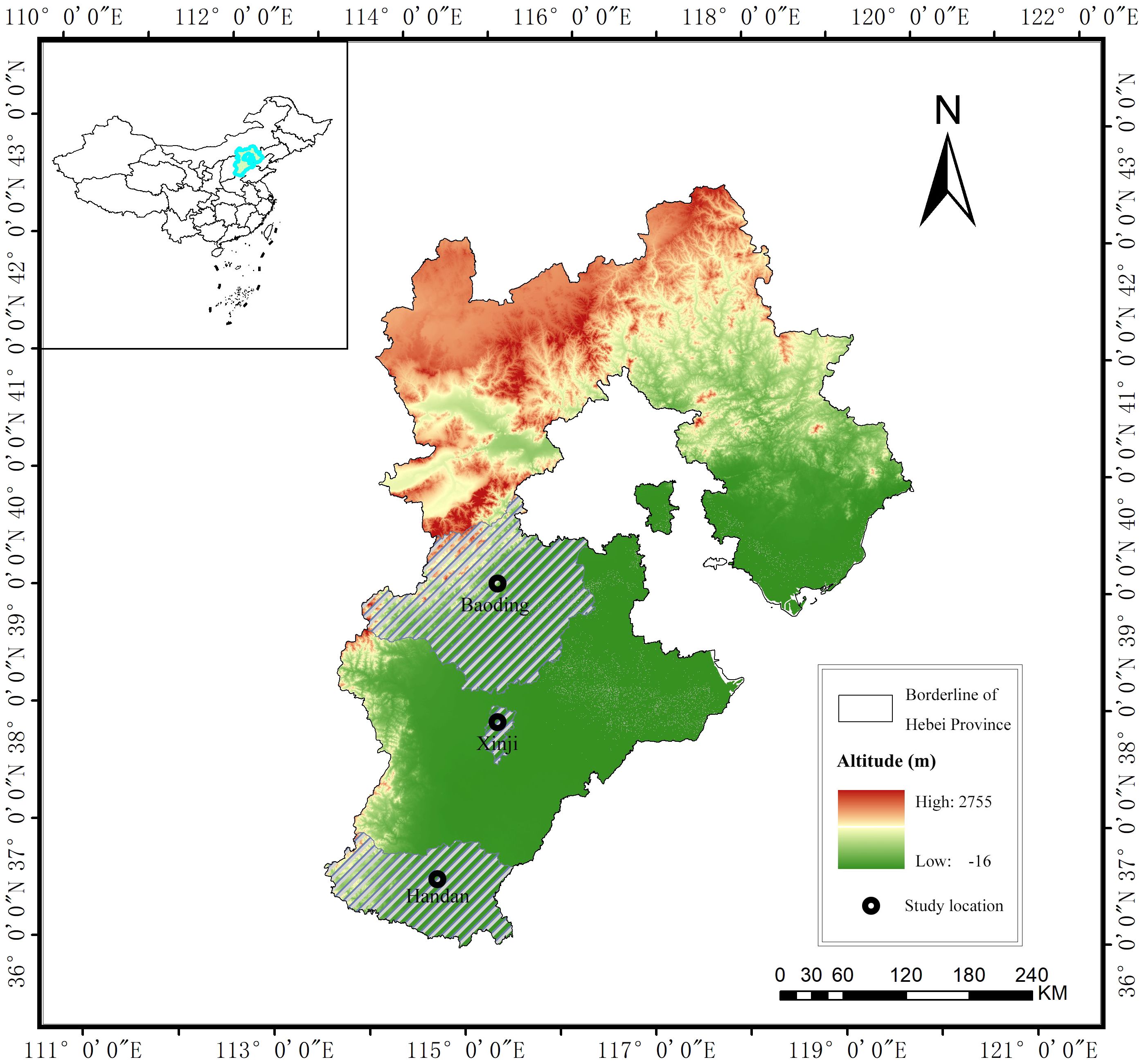
Figure 1 Study area.

2.2 Data preparation

The study is conducted in Baoding, Xinji, and Handan cities in Hebei Province, China. Meteorological data were sourced from the Meteorological Information Center of the National Meteorological Administration (http://www.nmic.cn/). The time span covered by the meteorological data is 1991–2019 for Baoding, 2000–2021 for Xinji, and 1991–2019 for Handan. The comprehensive meteorological datasets encompass information such as station name, elevation of the meteorological station, observation time, mean barometric pressure, mean water vapor pressure, mean air temperature, daily maximum temperature, daily minimum temperature, mean relative humidity, 8–8-h rainfall (24-h cumulative rainfall from 8 a.m. to 8 a.m. the next day), mean wind speed, and sunshine hours.

2.3 Selection of typical hydrological years

To mitigate the impact of annual rainfall variations on ET model estimation, a specific hydrological year was carefully chosen for the test area. Separate validations were conducted for each identified typical hydrological year to uphold model accuracy. The selection of typical hydrological years followed a process whereby cumulative annual rainfall data for Baoding City (1991–2019), Xinji City (2000–2021), and Handan City (1991–2019) underwent frequency exclusion. The annual rainfall was then ranked in descending order, and cumulative frequencies were computed for accurate year selection.

$\begin{array}{ll}\mathit{p}=\mathit{m}/(\mathit{N}+\mathbf{1})& (1)\end{array}$

where p represents the cumulative frequency, m is the ordinal number of years for rainfall after the treatment of rainfall frequency ranking, and N is the total number of years of rainfall. Utilizing the Pearson Type III curve for fitting, the rainfall values corresponding to p = 25%, 50%, 75%, and 90% are typically considered as the design values for high flow, median water, low flow, and special dry years.

2.4 ET₀ calculation method

The Haihe Plain region experiences four distinct seasons, marked by significant climatic variations. To assess the calculation accuracy of different ET₀ models during each fertility period of crops, daily ET₀ values for each identified typical hydrological year were computed using five ET₀ models, calculating daily ET₀ values for each typical hydrological year using five ET₀ models, and further obtaining monthly and 10-day ET₀ values.

(1) The Penman-Monteith model

The meteorological data utilized in the model encompass insolation, radiation, temperature, humidity, and wind speed. The Penman-Monteith equations are formulated to accurately predict ET₀ across diverse locations and climatic conditions, although they exhibit high demands for meteorological data. Previous studies applied the Penman-Monteith model in controlled environments (Doorenbos, 1977; Smith et al., 1991), emphasizing the importance of determining evaporative losses in the presence of various natural and anthropogenic land cover interventions. This approach aids in identifying the contributors to evaporative losses. The FAO Penman-Monteith model employed in this study is derived from the original Penman-Monteith equation, aerodynamic drag equation, and surface drag equation, as follows:

$\begin{array}{ll}\mathit{E}{\mathit{T}}_{\mathbf{0}}=\frac{\mathbf{0.408}\mathbf{\Delta }({\mathit{R}}_{\mathit{n}}-\mathit{G})+\mathit{\gamma }\frac{\mathbf{900}}{\mathit{T}+\mathbf{273}}{\mathit{u}}_{\mathbf{2}}({\mathit{e}}_{\mathit{s}}-{\mathit{e}}_{\mathit{a}})}{\mathbf{\Delta }+\mathit{\gamma }(\mathbf{1}+\mathbf{0.34}{\mathit{u}}_{\mathbf{2}})}& (2)\end{array}$

where R_n is the net radiation at the crop surface (MJ m^-2 day^-1), G is the soil heat flux (MJ m⁻² day⁻¹), T is the air temperature at a height of 2 m (°C), u₂ is the wind speed at a height of 2 m (ms⁻¹), e_s is the saturated water vapor pressure (kPa), e_a is the actual water vapor pressure (kPa), e_s − e_a is the difference in saturated water vapor pressure (kPa), Δ is the slope vapor pressure curve (kPa °C⁻¹), and γ is the psychrometric constant (kPa °C⁻¹).

(2) The Priestly-Taylor model

The meteorological data utilized in the model consist of insolation, radiation, and temperature (Priestley and Taylor, 1972). The PT model establishes a relationship between heat flux and evaporation. Notably simpler than the PM model, it eliminates the need for wind speed and humidity data, rendering it more convenient for application over large areas. However, subsequent studies have indicated that the PT model is better suited for humid areas (Priestley and Taylor, 1972; Pereira et al., 2007) and may not perform as well in arid regions. The formula is as follows:

$\begin{array}{ll}\mathit{E}{\mathit{T}}_{\mathbf{0}}=\mathit{\alpha }\frac{\mathbf{\text{Δ}}}{\mathbf{\Delta }+\mathit{\gamma }}({\mathit{R}}_{\mathit{n}}-\mathit{G}) & (3)\end{array}$

where α coefficient is mainly considered the influence of aerodynamic factors, in general, taking 1.26; Δ is the slope vapor pressure curve (kPa °C⁻¹), γ is the psychrometric constant (kPa °C⁻¹), R_n is the net radiation on the surface of the crop (MJ m⁻² day⁻¹), and G is the heat flux of the soil (MJ m⁻² day⁻¹).

(3) The Hargreaves model

The Hargreaves model, introduced by Hargreaves and Samani (Hargreaves and Samani, 1985), simplifies the estimation of ET₀. This model necessitates only the average daily maximum and minimum temperatures along with solar zenith radiation (Hargreaves and Allen, 2003), thereby reducing the need for extensive raw data. This characteristic makes it feasible to utilize observations for estimating ET₀ in regions where meteorological data are limited. The formula is as follows:

$\begin{array}{ll}\mathit{E}{\mathit{T}}_{\mathbf{0}}={\mathit{C}}_{\mathbf{0}}{\mathit{R}}_{\mathit{a}}({\mathit{T}}_{\mathit{m}\mathit{e}\mathit{a}\mathit{n}}+\mathbf{17.8})\sqrt{{\mathit{T}}_{\mathit{m}\mathit{a}\mathit{x}}-{\mathit{T}}_{\mathit{m}\mathit{i}\mathit{n}}}& (4)\end{array}$

where T_mean, T_max, and T_min represent the daily mean, daily maximum, and daily minimum temperatures, respectively; R_a is the atmospheric upper boundary solar radiation; and C₀ is the conversion factor, taken as 0.0023.

(4) The Mc-Cloud model

The Mc-Cloud model, introduced by McCloud in 1955, offers a simplified equation for estimating ET₀ based solely on temperature (McCloud, 1955). The formula is as follows:

$\begin{array}{ll}\mathit{E}{\mathit{T}}_{\mathbf{0}}=\mathit{K}{\mathit{W}}^{\mathbf{1.8}{\mathit{T}}_{\mathit{m}\mathit{e}\mathit{a}\mathit{n}}}& (5)\end{array}$

where K and W are constant terms, 0.254 and 1.07, respectively, and T_mean is the average temperature, °C.

(5) The FAO-24 Radiation model

The FAO-24 Radiation model, derived from the Makkink formula (Hauser et al., 1999), calculates ET₀ exclusively from solar radiation data. The formula is as follows:

$\begin{array}{ll} \mathit{E}{\mathit{T}}_{\mathbf{0}}=\mathit{a}+\mathit{b}\left(\frac{\mathbf{\Delta }}{\mathbf{\Delta }+\mathit{{\rm Y}}}{\mathit{R}}_{\mathit{s}}\right) & (6)\end{array}$

where a and b are empirical coefficients with values of 0.18 and 0.50, respectively; Δ is the slope vapor pressure curve (kPa °C⁻¹); γ is the psychrometric constant (kPa °C⁻¹), and R_s is the incoming short wave solar radiation, (MJ·m⁻²·day⁻¹).

2.5 Modifying evapotranspiration models using Bayesian estimation

The ET₀ values for each typical hydrological year were computed using the aforementioned five ET₀ models (Equations 2–6). Simulated values from the PM model served as the standard for analyzing the performance of the H-A, PT, F-R, and M-C models. The objective is to identify the most suitable and recommended model for simplified ET₀ estimation in the Haihe Plain region. Employing Bayesian theory, which involves both prior and posterior distributions, possible outcomes were obtained by reestimating the probability of an event occurring based on estimates of existing data. Bayesian estimation was iteratively applied to infer the model parameters, correcting the empirical parameters of the ET model. This iterative process enhances the model’s adaptability and accuracy in the study area.

2.6 Model performance statistics

Utilizing the original eight meteorological data inputs (daily minimum temperature, daily maximum temperature, daily average temperature, geographic latitude and longitude, altitude, average relative humidity, actual sunshine duration, and wind speed), the ET₀ inputs of the PM model were selected as the model’s calibration values. Statistical measures, including the R², RMSE, MAE, and WI (Equations 7–10) were employed as key factors for evaluating the model. These evaluation metrics are calculated as follows:

$\begin{array}{ll}{\mathit{R}}^2={\left[\frac{{\displaystyle {\sum }_{\mathit{i}=\mathbf{1}}^{\mathit{N}}({\mathit{P}}_{\mathit{i}}-\overline{\mathit{P}})({\mathit{Q}}_{\mathit{i}}-\overline{\mathit{Q}})}}{\sqrt{{\displaystyle {\sum }_{\mathit{i}=\mathbf{1}}^{\mathit{N}}{({\mathit{P}}_{\mathit{i}}-\overline{\mathit{P}})}^{\mathbf{2}}}}-\sqrt{{\displaystyle {\sum }_{\mathit{i}=\mathbf{1}}^{\mathit{N}}{({\mathit{Q}}_{\mathit{i}}-\overline{\mathit{Q}})}^{\mathbf{2}}}}}\right]}^{\mathbf{2}}& (7)\end{array}$

$\begin{array}{ll}\mathit{R}\mathit{M}\mathit{S}\mathit{E}=\sqrt{\frac{\mathbf{1}}{\mathit{N}}{\displaystyle {\sum }_{\mathit{i}=\mathbf{1}}^{\mathit{N}}{({\mathit{P}}_{\mathit{i}}-{\mathit{Q}}_{\mathit{i}})}^{\mathbf{2}}}}& (8)\end{array}$

$\begin{array}{ll}\mathit{M}\mathit{A}\mathit{E}=\frac{1}{\mathit{N}}{\displaystyle {\sum }_{\mathit{i}=\mathbf{1}}^{\mathit{N}}\left|{\mathit{P}}_{\mathit{i}}-{\mathit{Q}}_{\mathit{i}}\right|}& (9)\end{array}$

$\begin{array}{ll}\mathbf{\text{WI}}=\mathbf{1}-\frac{{\displaystyle {\sum }_{\mathit{i}=\mathbf{1}}^{\mathit{N}}{({\mathit{Q}}_{\mathit{i}}-{\mathit{P}}_{\mathit{i}})}^2}}{{\displaystyle {\sum }_{\mathit{i}=\mathbf{1}}^{\mathit{N}}{(\left|{\mathit{Q}}_{\mathit{i}}-\overline{\mathit{P}}\right|+\left|{\mathit{P}}_{\mathit{i}}-\overline{\mathit{P}}\right|)}^{\mathbf{2}}}}& (10)\end{array}$

where N is the number of data series; P_i and Q_i (mm/d) are the simulated and PM model ET₀ values, respectively; and $\overline{P}$ and $\overline{Q}$ (mm/day) are the average of the simulated and PM model ET₀ values, respectively.

3 Results and analysis

3.1 Selection of hydrological year

Based on the rainfall data from Baoding (1991–2019), Xinji (2000–2021), and Handan (1991–2019), the selection of typical hydrological years was carried out sequentially using Equation 1. The identified years for Baoding are 2008, 2009, 1992, and 1997, representing the high flow year (p = 25%), median water year (p = 50%), low flow year (p = 75%), and special dry year (p = 90%), respectively. Similarly, for Xinji, the years are 2004, 2010, 2007, and 2006, and for Handan, the years are 1993, 2014, 2006, and 2017, corresponding to the same hydrological conditions (Figure 2 and Table 1).

Figure 2

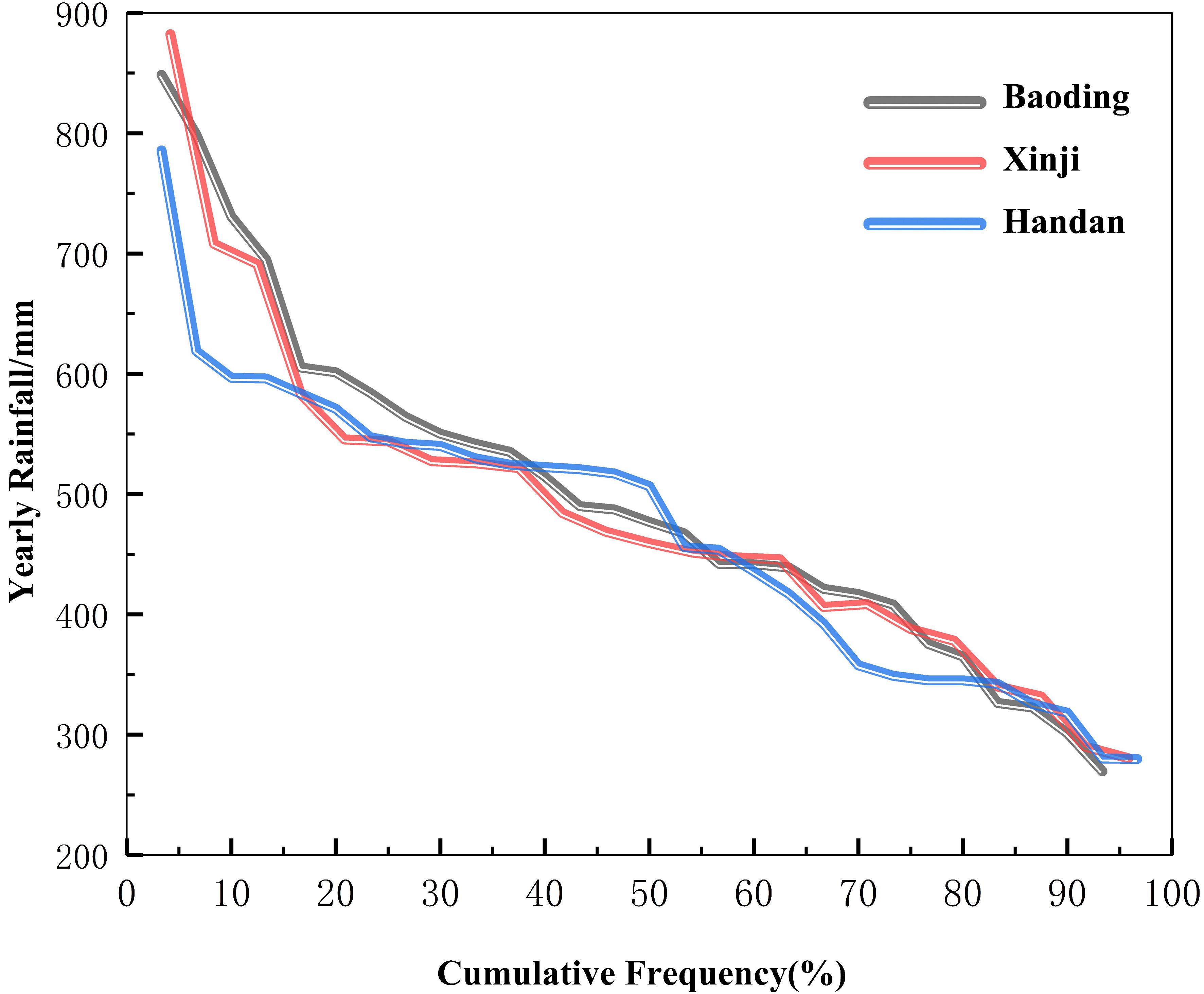
Figure 2 Typical hydrological year selection.

Table 1

Table 1 Selection of typical hydrological years in some areas of the Haihe Plain region.

3.2 Comparative analysis of daily ET₀ values for different typical hydrologic years

In Figure 3, the day-by-day ET₀ trends of the five models across the three regions under various typical hydrological years exhibit patterns approximating monotonically increasing and decreasing parabolas. The upward segment spans from January to July, followed by a downward segment from July to December, with peak values occurring in the months of June and July for all five models. Comparatively, the H-A model consistently produces higher ET₀ results than the PM model throughout the year. In contrast, the PT and F-R models consistently yield lower ET₀ results than the PM model throughout the year. The M-C model produces higher ET₀ results than the PM model in the months of June–September but lower values in the remaining months.

Figure 3

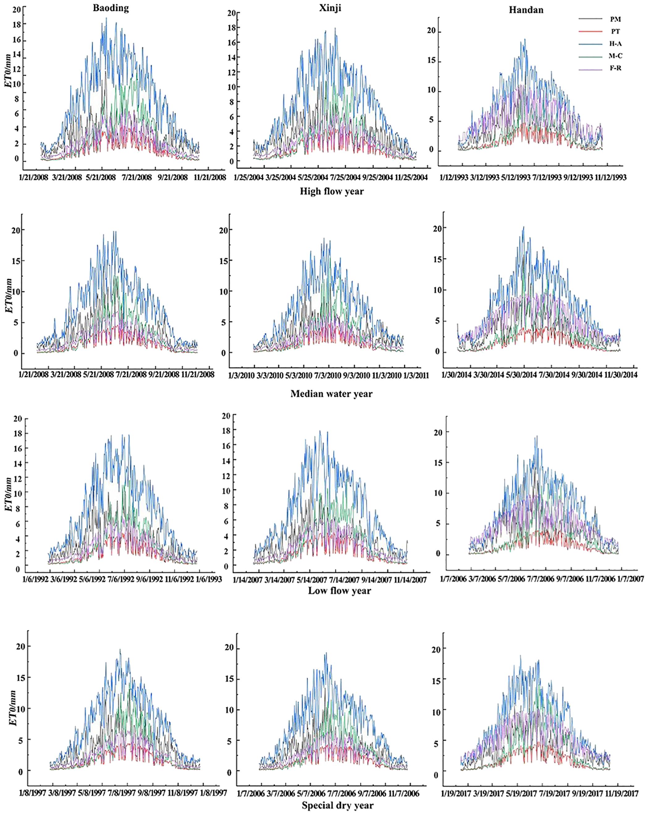
Figure 3 ET₀ values of different models under typical hydrological year at daily scale.

Using the PM model-calculated ET₀ values as the standard, a comparative analysis of daily ET₀ values for the remaining four ET models is conducted under different typical hydrological years. At the daily scale, the H-A model yielded slightly larger results than the PM model while the F-R and PT models produced slightly lower values. The remaining three models showed relatively close results to the PM model, except for the H-A model. The PM model and the other four models were used to calculate the RMSE, MAE, and R² for each typical hydrological year. The results are presented in Table 2. At a significance level of 0.01, the PT, H-A, and F-R models exhibited good correlation with the PM model’s standard values. The average R² for PT, H-A, and F-R models in typical hydrological years were 0.710, 0.703, and 0.748 in Baoding; 0.707, 0.718, and 0.746 in Xinji; and 0.644, 0.664, and 0.644 in Handan, respectively. All three models had R²>0.6, demonstrating their predictive effectiveness at the daily scale. However, the M-C model showed an average R² of 0.500, 0.480, and 0.471 in Baoding, Xinji, and Handan, respectively, with R²<0.6, indicating a lower prediction effectiveness. Moreover, in each typical hydrological year, the F-R model consistently exhibits smaller RMSE and MAE compared with the PT and H-A models. Moreover, the WI is higher for the F-R model, indicating its superior predictive performance for daily ET₀ values under varying hydrological conditions.

Table 2

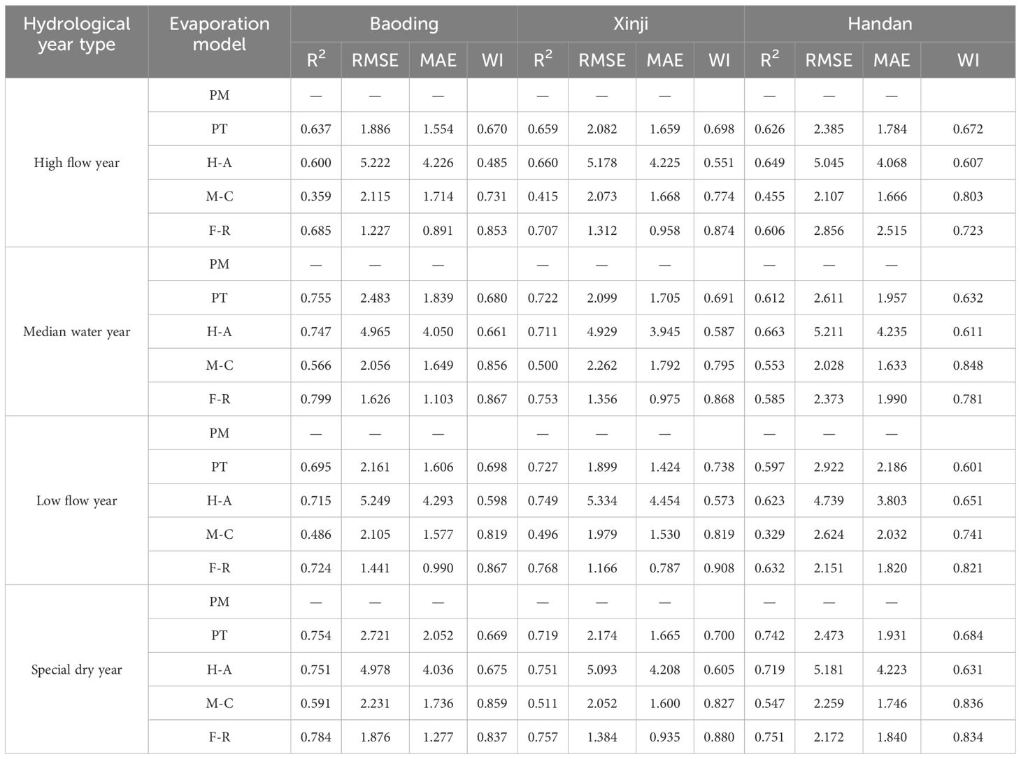
Table 2 Comparison the performances of different models under typical hydrological year at daily scale.

3.3 Comparative analysis of monthly ET₀ values for different typical hydrologic years

In Figure 4, the monthly ET₀ trends of the five models across the three regions under various typical hydrological years exhibit patterns resembling monotonically increasing and decreasing parabolas. The upward segment spans from January to July, followed by a downward segment from July to December, with peak values occurring in the months of June and July for all five models. Similar to the daily trends, the H-A model consistently produces higher ET₀ results than the PM model throughout the year. In contrast, the PT and F-R models consistently yield lower ET₀ results than the PM model throughout the year. The M-C model produces higher ET₀ results than the PM model in the months of June–September but lower values in the remaining months.

Figure 4

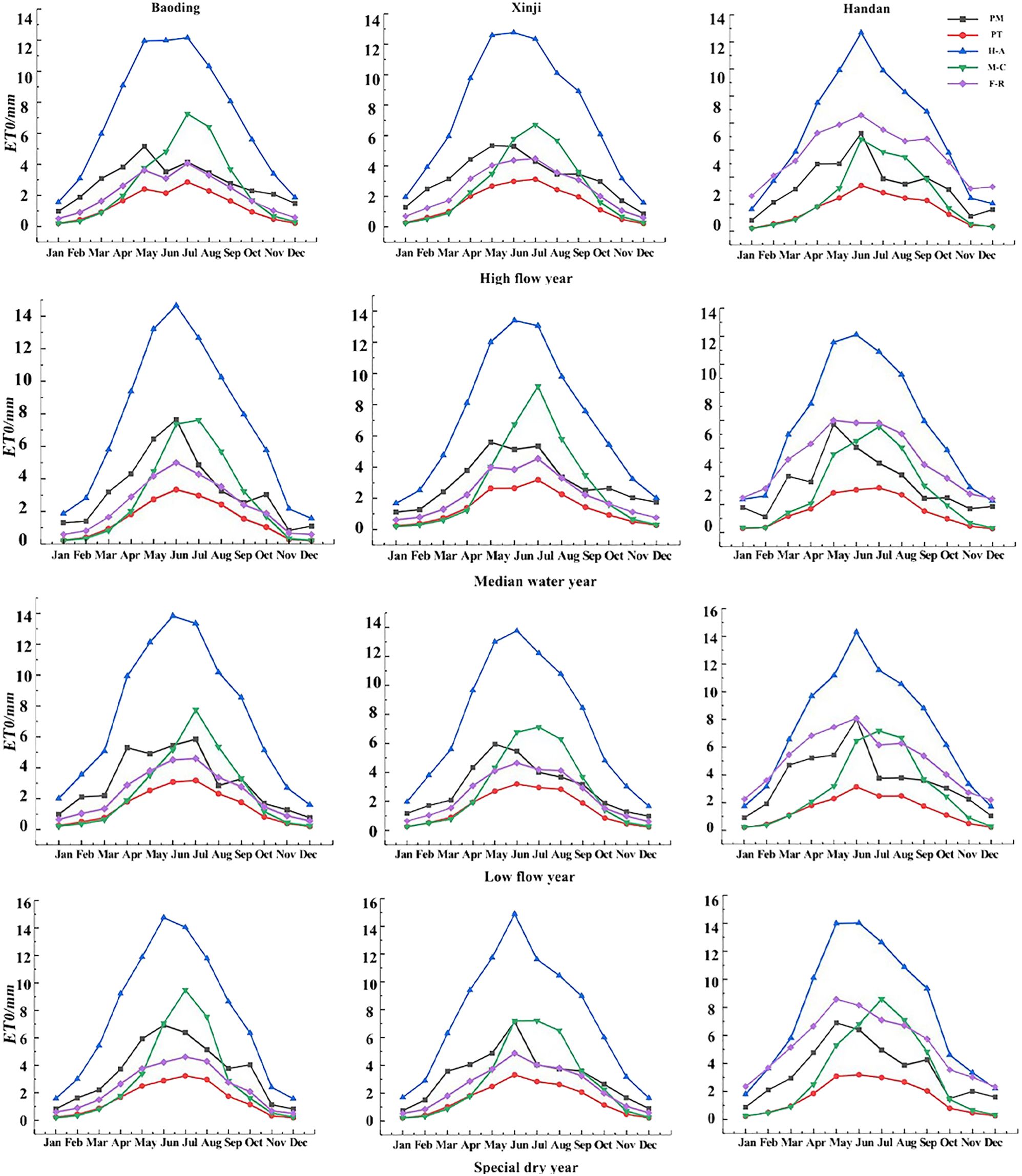
Figure 4 ET₀ values of different models under typical hydrological year at monthly scale.

Using the PM model-calculated ET₀ values as the standard, a comparative analysis of monthly ET₀ values for the remaining four ET₀ models is conducted under different typical hydrological years. At the monthly scale, the H-A model yielded slightly larger results than the PM model while the F-R and PT models produced slightly lower values. The remaining three models showed relatively close results to the PM model, except for the H-A model. The PM model and the other four models were used to calculate the RMSE, MAE, and R² for each typical hydrological year. The results are presented in Table 3. At a significance level of 0.01, the PT, H-A, and F-R models exhibited good correlation with the PM model’s standard values. The average R² for PT, H-A, and F-R models in typical hydrological years were 0.852, 0.900, and 0.879 for Baoding, Xinji, and Handan, respectively. All three models had R² > 0.8, indicating better prediction effects at the monthly scale. However, the M-C model showed an average R² of 0.622, 0.607, and 0.554 in Baoding, Xinji, and Handan, respectively, with R² around 0.6, signifying poorer prediction compared with other models. Simultaneously, in each typical hydrological year, the F-R model consistently exhibits smaller RMSE and MAE compared with the PT and H-A models. Additionally, the WI is higher for the F-R model, indicating its superior predictive performance for monthly ET₀ values under varying hydrological years.

Table 3

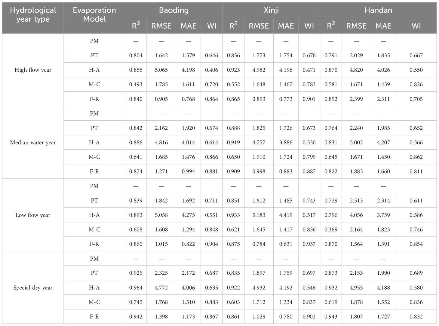
Table 3 Comparison the performances of different models under typical hydrological year at monthly scale.

3.4 Comparative analysis of 10-day ET₀ values for different typical hydrologic years

In Figure 5, the trends of 10-day ET₀ values from the five models across the three regions under various typical hydrological years exhibit patterns resembling monotonically increasing and decreasing parabolas. The overall trend indicates an increase from January to around early July and a subsequent decrease from around early July to the end of December, with peak values occurring around early June to early July. Similar to the daily and monthly trends, the H-A model consistently produces higher ET₀ results than the PM model throughout the year. In contrast, the PT and F-R models consistently yield lower ET₀ results than the PM model throughout the year. The M-C model produces higher ET₀ results than the PM model from mid-late June to early September, and the remaining 10-day ET₀ values are lower than those of the PM model.

Figure 5

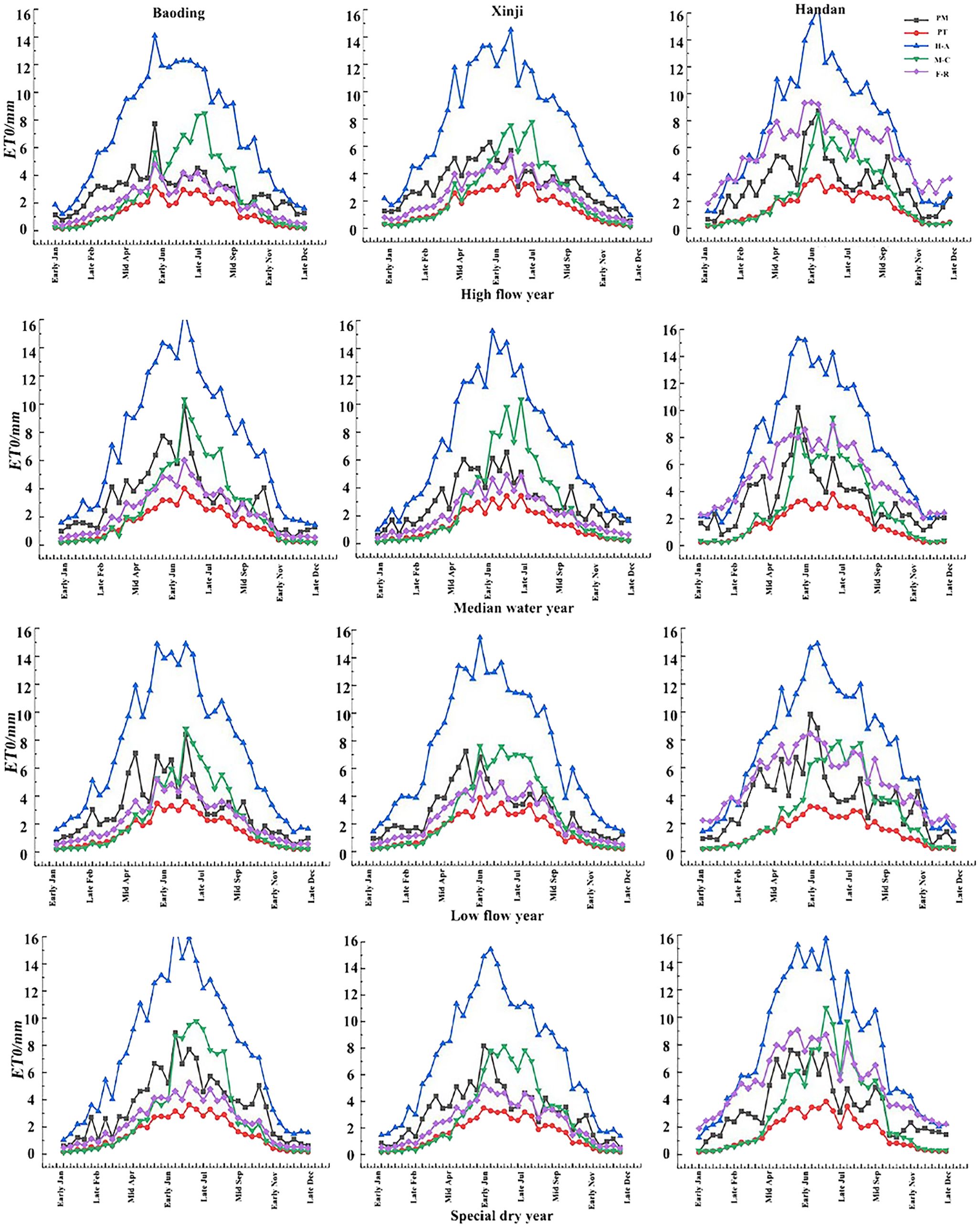
Figure 5 ET₀ values of different models under typical hydrological year at the ten-day scale.

Using the PM model-calculated ET₀ values as the standard, a comparative analysis of 10-day ET₀ values for the remaining four ET₀ models is conducted under different typical hydrological years. At the 10-day scale, the results of the H-A model are slightly larger than the standard value of the PM model, the results of the F-R model and the PT model are slightly lower than the standard value of the PM model, and the results of the other three models are relatively close to those of the PM model except for the H-A model. The PM model and the other four models were used to calculate the RMSE, MAE, and R² for each typical hydrological year, and their corresponding results were analyzed. The results are shown in Table 4. At significance of 0.01, the analytical results of the three models, PT, H-A, and F-R, have good correlation with the standard values of the PM model, among which the average coefficients of determination (R²) of the three models, PT, H-A, and F-R, in typical hydrological years are 0.806, 0.835, and 0.840 in Baoding, Xinji, and Handan cities, respectively; 0.818, 0.885, and 0.851, respectively; and 0.743, 0.799, and 0.815 respectively. The R² of the three models is >0.8, which proves that the three models have better prediction effects at the decadal scale. In contrast, the average coefficients of determination (R²) of the M-C model were 0.593, 0.560, and 0.521 in Baoding, Xinji, and Handan, respectively, with R²< 0.6, and the model predicted poorly. Meanwhile, during each typical hydrological year, the F-R model consistently demonstrates smaller RMSE and MAE in comparison with the PT and H-A models. Furthermore, the F-R model exhibits a higher WI, implying superior predictive accuracy for 10-day ET₀ values across varying hydrological years.

Table 4

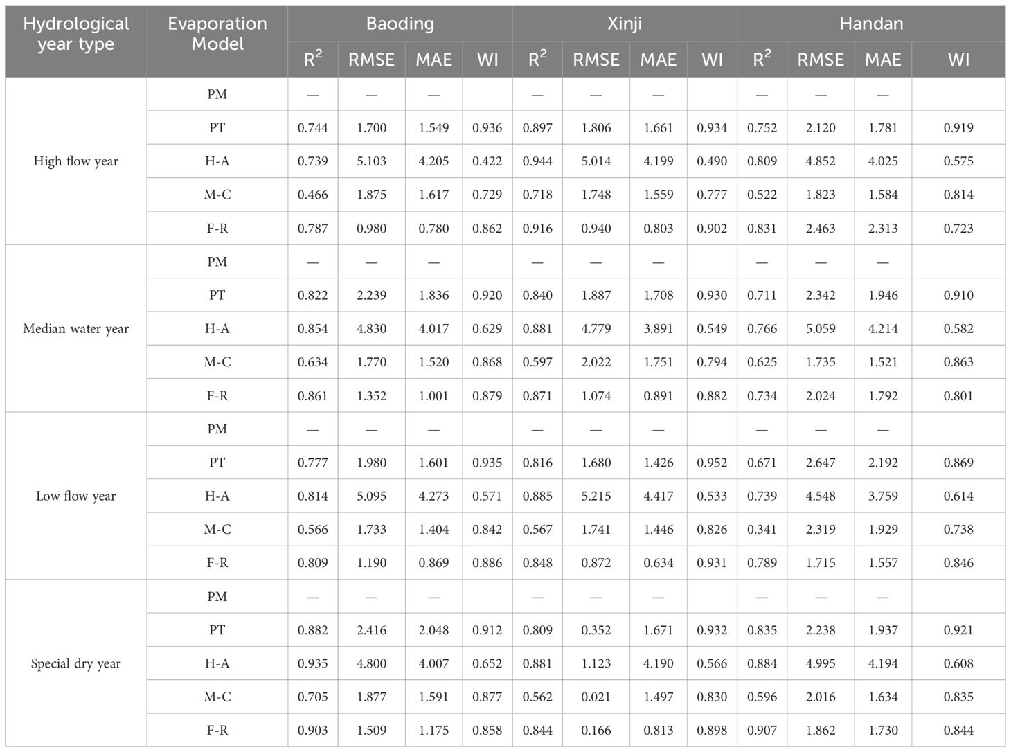
Table 4 Comparison the performances of different models under typical hydrological year at 10-day scale.

In conclusion, among the three models analyzed (PT, H-A, and F-R), all show predictive ability under different typical hydrological years, excluding the M-C model. The PT model demonstrates good correlation at daily, monthly, and 10-day scales across different regions. Specifically, the daily scale R² in Baoding, Xinji, and Handan are 0.710, 0.707, and 0.644, respectively; the monthly scale R² are 0.852, 0.852, and 0.789, respectively; and the 10-day scale R² are 0.806, 0.818, and 0.743, respectively. The H-A model exhibits better correlation at different scales with daily scale R² values in Baoding, Xinji, and Handan of 0.703, 0.718, and 0.664, respectively. The monthly scale R² are 0.900, 0.924, and 0.857, while the 10-day scale R² are 0.835, 0.885, and 0.799. However, the H-A model has larger RMSE and MAE values compared with the PT and F-R models, indicating higher prediction errors.

The F-R model shows good correlation at different scales with daily scale R² values in Baoding, Xinji, and Handan of 0.748, 0.746, and 0.644, respectively. The monthly scale R² are 0.879, 0.877, and 0.822, while the 10-day scale R² are 0.840, 0.851, and 0.815. Compared with other models, the F-R model demonstrates higher R² values, along with lower RMSE and MAE. Additionally, its WI is consistently higher across various time scales. Consequently, the F-R model shows superior applicability in the Haihe Plain region, particularly after correction, making it more suitable for predicting ET₀ in this area.

3.5 FAO-24 Radiation improvement

The Bayesian estimation method is utilized to iteratively infer the empirical parameters a and b in the F-R model, leveraging meteorological data from Baoding City (1991–2014), Xinji City (2000–2016), and Handan City (1991–2014). The process entails computing posterior distributions of coefficient b using prior data, followed by iteratively calculating coefficient a by incorporating adjusted b values into the prior data. This iterative procedure refines model parameters, enhancing the accuracy of ET₀ estimation. The specific procedure is as follows:

In accordance with the original F-R model, the two parameters can be expressed as:

$\begin{array}{ll}\mathit{b}=\frac{\mathit{E}{\mathit{T}}_{\mathbf{0}}-\mathit{a}}{\frac{\text{Δ}}{\text{Δ}+\mathit{{\rm Y}}}{\mathit{R}}_{\mathit{s}}}& (11)\end{array}$

$\begin{array}{ll} \mathit{a}=\mathit{E}{\mathit{T}}_{\mathbf{0}}-\mathit{b}\frac{\text{Δ}}{\text{Δ}+\mathit{{\rm Y}}}{\mathit{R}}_{\mathit{s}}& (12)\end{array}$

(2) The distribution of b and a values follows a normal distribution. The coefficient b was calibrated using Equations 11-13 using day-by-day meteorological data for a typical hydrological year.

$\begin{array}{ll} \mathit{E}=\frac{{\mathit{\alpha }}_{\mathit{o}}\widehat{{\mathit{\delta }}^{\mathbf{2}}}+\widehat{\mathit{\Theta }}{\mathbf{0.81}}^{\mathbf{2}}}{\widehat{{\mathit{\delta }}^{\mathbf{2}}}+{\mathbf{0.81}}^{\mathbf{2}}}& (13)\end{array}$

where E is the mathematical expectation, ${\alpha }_o$ is the corresponding initial value, and $\widehat{\text{Θ}}$ is the estimated mean as well as the variance $\widehat{{\mathit{\delta }}^{\mathbf{2}}}$. Following the same procedure, the mathematical expectation of a is calculated by Equation 12 and Equation 13. The obtained expectations of parameters b and a are substituted into the F-R model in order to obtain the Calibrated F-R model as shown in Table 5.

Table 5

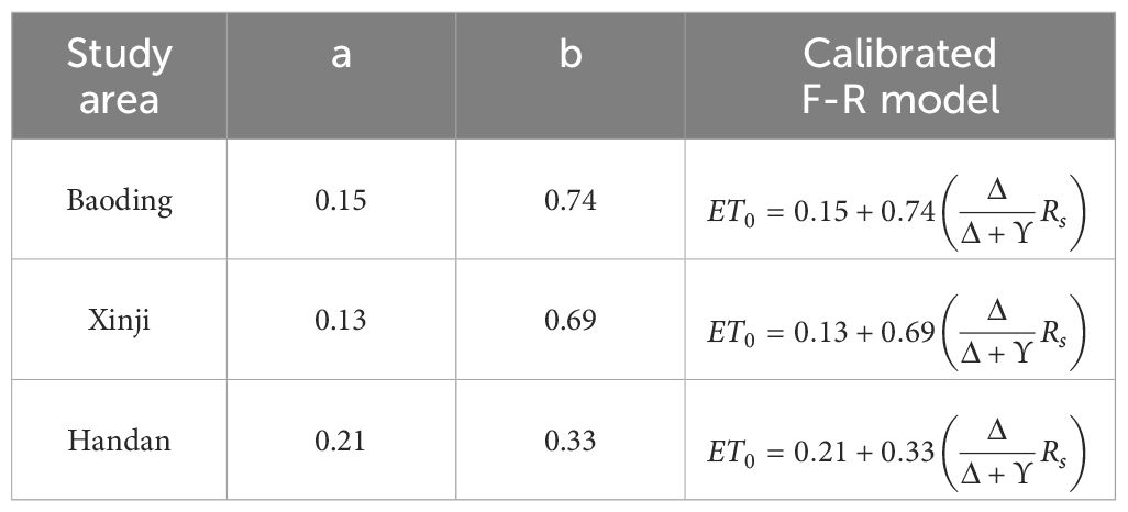
Table 5 F-R correction model.

3.6 Validation of improved F-R model

Following Shiri et al.’s recommendation (Shiri et al., 2015), validation with a distinct dataset was employed to ensure unbiased results. The original and calibrated models were evaluated using meteorological data from Baoding and Handan (2015–2019) and Xinji (2017–2021). ET₀ values were computed for both monthly and 10-day periods derived from the daily values.

After comparing the error analysis results in Table 6 and Table 7, it is evident that under a significance level of P < 0.01, R² remained unchanged. However, Figure 6 shows significant decreases in RMSE and MAE across daily, monthly, and 10-day scales, accompanied by further improvements in WI. In Baoding City, Xinji City, and Handan City, the average coefficients of determination (R²) at the daily scale are 0.632, 0.746, and 0.693, respectively. At the monthly scale, the average R² values are 0.769, 0.871, and 0.905, respectively, and at the 10-day scale, the average R² values are 0.790, 0.838, and 0.852, respectively. There is good correlation at all three scales. Comparing the ET₀ values before and after modification, the modified F-R model reduced RMSE by 15.81%, 29.51%, and 24.66% at the daily, monthly, and 10-day scales, respectively. MAE decreased by 19.04%, 34.47%, and 28.52% at the daily, monthly, and 10-day scales, respectively, while WI increased by 5.49%, 8.48%, and 10.78% at the daily, monthly, and 10-day scales, respectively. Therefore, the modified model can be effectively used for calculating reference crop evapotranspiration in the Haihe Plain region.

Figure 6

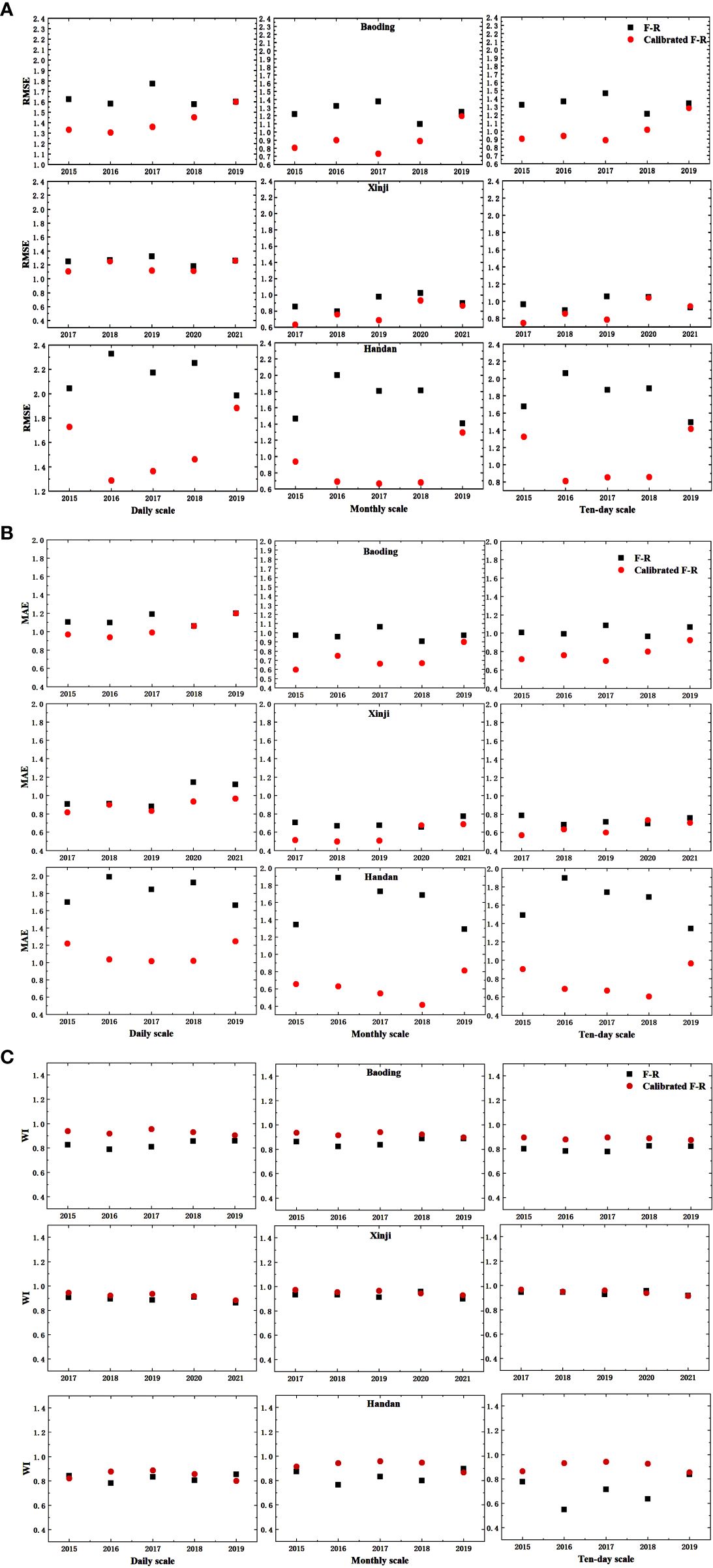
Figure 6 The comparisons of RMSE, MAE, and WI before and after the F-R model calibrated; (A) RMSE; (B) MAE; (C) WI.

Table 6

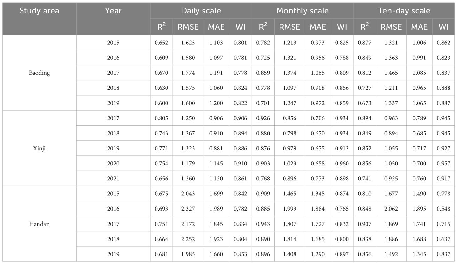
Table 6 Error analysis of the original F-R model.

Table 7

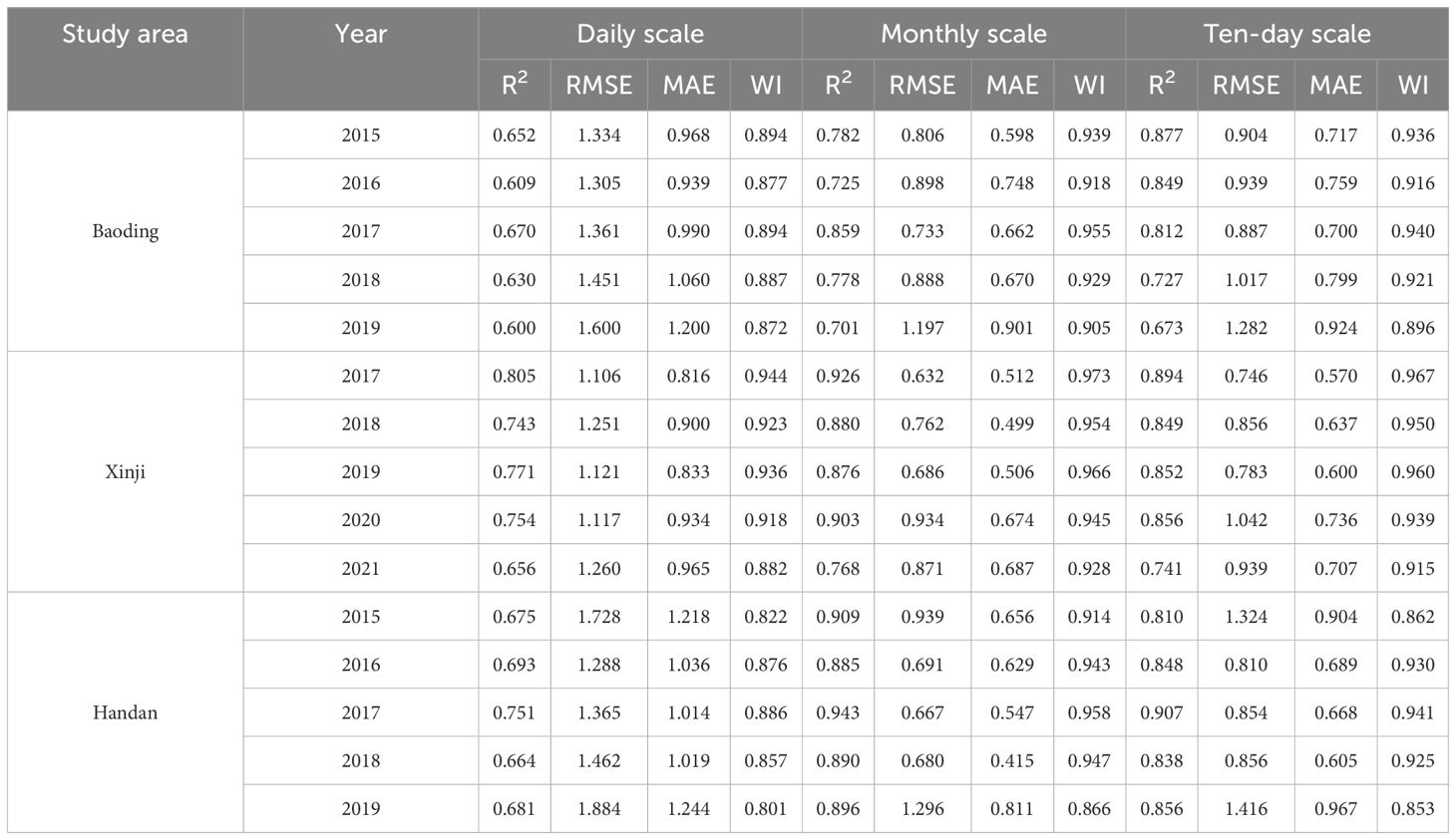
Table 7 Error analysis of the calibrated F-R model.

4 Discussion

This study compared and evaluated the applicability of four evapotranspiration models—Priestley-Taylor (PT), Hargreaves (H-A), Mc-Cloud (M-C), and FAO-24 Radiation (F-R)—that use incomplete meteorological data. The Penman-Monteith (PM) model’s ET₀ values were used as a benchmark for comparison. Overall, the simulation results highlight the superior performance of the F-R model among the four models.

The F-R model calculates ET₀ mainly based on solar radiation data (Hauser, Gimon, Horin, & TX, 1999), which mainly uses the actual sunshine duration to obtain the solar magnetic declination, the atmospheric upper boundary solar radiation, and thus further the actual solar radiation. By analyzing the results of this study, under the condition of incomplete meteorological data, the simulated values of the F-R model at three scales of daily, monthly, and decadal under different typical hydrological years in three areas of the Haihe Plain before the modification have good correlation with the standard values of the PM model, and the results of the error analyses are also satisfactory. By further correcting the F-R model calculations, as shown in Table 6 and Table 7, the R² of the corrected F-R model did not change at a significance level of P < 0.01, whereas the RMSE and the MAE in the study area decreased substantially. Therefore, the predictions of the modified F-R model were more satisfactory and can be used for the calculation of ET of local reference crops.

The use of historical data for model calibration may lead to instability over time due to changing climate conditions. To address this, a suitable calibration method is essential. In this study, the simulated values of the Penman-Monteith (PM) model were employed as standards for the comparative analysis of four models: Priestly-Taylor (PT), Hargreaves (H-A), Mc-Cloud (M-C), and FAO-24 Radiation (F-R). The F-R model was identified as the most suitable for the Haihe Plain region with incomplete meteorological data. Considering geographical differences in the original F-R model’s applicability, a modification was performed using the Bayesian principle. This method utilizes known data as the prior distribution and recalculates data as the new posterior distribution, improving the reliability of the calculation by overcoming empirical data uncertainty and considering spatial-temporal variability. The Bayesian approach ensures a systematic and adaptive calibration method, enhancing stability and reliability in different scenarios. Beck et al. introduced Bayesian theory into model correction for the first time and clarified the basic idea of the correction (Beck and Katafygiotis, 1998), and also put forward a kind of adaptive MH algorithm-based Markov chain Monte Carlo method based on the MH algorithm (Beck and Au, 2002). Cheung et al. introduced and improved the hybrid Monte Carlo (HMCMC) method to solve the problem of Bayesian model correction for high-dimensional uncertainty parameters (Cheung and Beck, 2009). Currently, there is a recommended application of the modified Hargreaves model using Bayesian estimation method to calculate the ET of de-measured reference crops in the Sichuan Basin area (Feng et al., 2017). The modification of the F-R model using the Bayesian principle in the experimental area ensures the model’s applicability, providing a more accurate ET₀ calculation. This enhanced model can serve as a scientific foundation for future farmland moisture management in the Haihe Plain area.

Different types of models have different sensitivities to meteorological data and are adapted to different regions. The PT model does not require wind speed and humidity data (Priestley and Taylor, 1972), and by comparing with the standard values of the PM model, the overall PT model simulation values are lower than those of the PM model, and the three scales of daily, monthly, and decadal are all well correlated under different typical hydrological years in the three regions of the Haihe Plain, and the error analysis. The results are relatively satisfactory. It can be used to calculate the ET₀ in the Haihe Plain if the error is within the allowable range. In contrast to the PM model method for calculating reference ET, the PT model ignores the effect of water vapor deficit on reference ET, thus generating the assumption that ET₀ depends only on solar radiation and temperature (Wu et al., 2021). This allows for PT modeling where PM modeling is not possible due to lack of data (Utset et al., 2004). It has been demonstrated that the simple and less data-demanding PT model is a good choice in many climatic regions (Jamieson, 1982; Pereira and Nova, 1992; Sau et al., 2004).

The M-C model is a simplified calculation method of ET₀ based on temperature (McCloud, 1955), which just uses the daily mean temperature as meteorological data, and by comparing with the standard value of PM model, the correlation of this model is low, R² < 0.6, indicating that this model is not good at predicting in the sea–river plain area. However, the M-C model is based on the daily mean air temperature, which is easy to calculate and especially suitable for areas with large differences in temperature variations (Valipour, 2015). The H-A model is suitable for the lack of radiative data and just uses the daily mean air temperature, daily maximum and daily minimum air temperature, and the atmospheric upper boundary solar radiation calculated through the daily ordinate. The simulated values of this model are compared with the PM model. The model simulated values are compared with the standard values of the PM model, and although there is a high correlation, the results of the error analysis are less satisfactory, with larger values of RMSE and MAE, and the model is not effective in predicting in the test area. However, many studies have confirmed that the H-A model is also a good predictor in some regions, and model optimization is continuously performed to better adapt to climate change (Gavilán et al., 2006; Tabari and Talaee, 2011; Berti et al., 2014; Cobaner et al., 2017). These calibrations are site-specific and cannot be extrapolated to some sites with completely different meteorological conditions.

This study warrants further validation, especially considering the absence of measured ET₀ data. While the PM model served as the standard for calibrating the F-R model based on Bayesian theory, it is essential to verify the conclusions with measured data. Relying solely on model calculations, as highlighted by Martí et al (Martí et al., 2015), may yield unreasonable or incorrect conclusions. Therefore, incorporating measured ET₀ data from lysimeters for calibration and evaluation is crucial. Moreover, while Bayesian theory allows for updating model parameters based on new sample data, it is important to note that this method is purely mathematical and overlooks the physical basis of the evapotranspiration process. Consequently, future research should emphasize calibrating the model using measured solar radiation data to enhance its accuracy.

5 Conclusions

In this study, we conducted a comparative analysis of four evapotranspiration models using incomplete meteorological data across various hydrological conditions to enhance ET₀ estimation accuracy. The results revealed consistent spatial distribution trends among the models, with the F-R model demonstrating superior accuracy and predictive performance, particularly in terms of R² and WI. Furthermore, the calibrated F-R model, refined through Bayesian theory, achieved higher accuracy, with R² reaching 0.85 and WI reaching 0.9. The calibrated FAO-24 Radiation model offers valuable insights for precise ET₀ estimation and irrigation decision-making in the Haihe Plain region, suggesting avenues for further accuracy improvements in future research.

Data availability statement

The original contributions presented in the study are included in the article/supplementary material. Further inquiries can be directed to the corresponding authors.

Author contributions

XS: Writing – review & editing, Writing – original draft, Visualization, Validation, Formal analysis, Data curation. BZ:Writing – original draft, Methodology, Data curation. MD:Visualization, Writing – original draft. RG: Writing – original draft, Visualization. CJ: Writing – original draft, Formal analysis. KM: Writing – original draft, Visualization. SG: Writing – original draft, Methodology. LG: Writing – review & editing, Supervision, Funding acquisition. WZ: Writing – review & editing, Supervision, Funding acquisition. XG: Methodology, Writing – review & editing, Supervision.

Funding

The author(s) declare financial support was received for the research, authorship, and/or publication of this article. This material is based on work supported by the Key R&D projects in Hebei Province (22326406D, 21327001D) and Foundation of State Key Laboratory of North China Crop Improvement and Regulation (NCCIR2021ZZ-24).

Conflict of interest

The authors declare that the research was conducted in the absence of any commercial or financial relationships that could be construed as a potential conflict of interest.

Publisher’s note

All claims expressed in this article are solely those of the authors and do not necessarily represent those of their affiliated organizations, or those of the publisher, the editors and the reviewers. Any product that may be evaluated in this article, or claim that may be made by its manufacturer, is not guaranteed or endorsed by the publisher.

References

Akumaga, U., Alderman, P. D. (2019). Comparison of penman–monteith and priestley-taylor evapotranspiration methods for crop modeling in Oklahoma. Agron. J. 111, 1171–1180. doi: 10.2134/agronj2018.10.0694

CrossRef Full Text | Google Scholar

Alam, M. M., Akter, M. Y., Islam, A. R. M. T., Mallick, J., Kabir, Z., Chu, R., et al. (2024). A review of recent advances and future prospects in calculation of reference evapotranspiration in Bangladesh using soft computing models. J. Environ. Manage. 351, 119714. doi: 10.1016/j.jenvman.2023.119714

PubMed Abstract | CrossRef Full Text | Google Scholar

Allen, R. G. (1998). Crop Evapotranspiration-Guideline for computing crop water requirements. Irrigation drain 56, 300.

Google Scholar

Allen, R. G., Pruitt, W. O., Wright, J. L., Howell, T. A., Ventura, F., Snyder, R., et al. (2006). A recommendation on standardized surface resistance for hourly calculation of reference ETo by the FAO56 Penman-Monteith method. Agric. Water Manage. 81, 1–22. doi: 10.1016/j.agwat.2005.03.007

CrossRef Full Text | Google Scholar

Almorox, J., Quej, V. H., Martí, P. (2015). Global performance ranking of temperature-based approaches for evapotranspiration estimation considering Köppen climate classes. J. Hydrology 528, 514–522. doi: 10.1016/j.jhydrol.2015.06.057

CrossRef Full Text | Google Scholar

Beck, J. L., Au, S.-K. (2002). Bayesian updating of structural models and reliability using Markov chain Monte Carlo simulation. J. Eng. mechanics 128, 380–391. doi: 10.1061/(ASCE)0733-9399(2002)128:4(380)

CrossRef Full Text | Google Scholar

Beck, J. L., Katafygiotis, L. S. (1998). Updating models and their uncertainties. I: Bayesian statistical framework. J. Eng. mechanics 124, 455–461. doi: 10.1061/(ASCE)0733-9399(1998)124:4(455)

CrossRef Full Text | Google Scholar

Berti, A., Tardivo, G., Chiaudani, A., Rech, F., Borin, M. (2014). Assessing reference evapotranspiration by the Hargreaves method in North-Eastern Italy. Agric. Water Manage. 140, 20–25. doi: 10.1016/j.agwat.2014.03.015

CrossRef Full Text | Google Scholar

Boretti, A., Rosa, L. (2019). Reassessing the projections of the world water development report. NPJ Clean Water 2, 15. doi: 10.1038/s41545-019-0039-9

CrossRef Full Text | Google Scholar

Cheung, S. H., Beck, J. L. (2009). Bayesian model updating using hybrid Monte Carlo simulation with application to structural dynamic models with many uncertain parameters. J. Eng. mechanics 135, 243–255. doi: 10.1061/(ASCE)0733-9399(2009)135:4(243)

CrossRef Full Text | Google Scholar

Chia, M. Y., Huang, Y. F., Koo, C. H., Fung, K. F. (2020). Recent advances in evapotranspiration estimation using artificial intelligence approaches with a focus on hybridization techniques—a review. Agronomy 10, 101. doi: 10.3390/agronomy10010101

CrossRef Full Text | Google Scholar

Choi, Y., Kim, M., O'Shaughnessy, S., Jeon, J., Kim, Y., Song, W. J. (2018). Comparison of artificial neural network and empirical models to determine daily reference evapotranspiration. J. Korean Soc. Agric. Engineers 60, 43–54. doi: 10.5389/KSAE.2018.60.6.043

CrossRef Full Text | Google Scholar

Cobaner, M., Citakoğlu, H., Haktanir, T., Kisi, O. (2017). Modifying Hargreaves–Samani equation with meteorological variables for estimation of reference evapotranspiration in Turkey. Hydrology Res. 48, 480–497. doi: 10.2166/nh.2016.217

CrossRef Full Text | Google Scholar

Dimitriadou, S., Nikolakopoulos, K. G. (2022). Artificial neural networks for the prediction of the reference evapotranspiration of the Peloponnese Peninsula, Greece. Water 14, 2027. doi: 10.3390/w14132027

CrossRef Full Text | Google Scholar

Doorenbos, J. (1977). Crop water requirements. FAO irrigation and drainage paper 24. Land and Water Development Division. Rome: FAO, 144 (1).

Google Scholar

Droogers, P., Allen, R. G. (2002). Estimating reference evapotranspiration under inaccurate data conditions. Irrigation drainage Syst. 16, 33–45. doi: 10.1023/A:1015508322413

CrossRef Full Text | Google Scholar

Elbeltagi, A., Nagy, A., Mohammed, S., Pande, C. B., Kumar, M., Bhat, S. A., et al. (2022). Combination of limited meteorological data for predicting reference crop evapotranspiration using artificial neural network method. Agronomy 12, 516. doi: 10.3390/agronomy12020516

CrossRef Full Text | Google Scholar

Feng, Y., Jia, Y., Cui, N., Zhao, L., Li, C., Gong, D. (2017). Calibration of Hargreaves model for reference evapotranspiration estimation in Sichuan basin of southwest China. Agric. Water Manage. 181, 1–9. doi: 10.1016/j.agwat.2016.11.010

CrossRef Full Text | Google Scholar

Food, & Nations, A. O. o. t. U (2017). The future of food and agriculture: Trends and challenges. (Fao). doi: 10.22004/ag.econ.319843

CrossRef Full Text | Google Scholar

Gao, L., Gong, D., Cui, N., Lv, M., Feng, Y. (2021). Evaluation of bio-inspired optimization algorithms hybrid with artificial neural network for reference crop evapotranspiration estimation. Comput. Electron. Agric. 190, 106466. doi: 10.1016/j.compag.2021.106466

CrossRef Full Text | Google Scholar

Gavilán, P., Lorite, I., Tornero, S., Berengena, J. (2006). Regional calibration of Hargreaves equation for estimating reference ET in a semiarid environment. Agric. Water Manage. 81, 257–281. doi: 10.1016/j.agwat.2005.05.001

CrossRef Full Text | Google Scholar

Gu, Z., Zhu, T., Jiao, X., Xu, J., Qi, Z. (2021). Neural network soil moisture model for irrigation scheduling. Comput. Electron. Agric. 180, 105801. doi: 10.1016/j.compag.2020.105801

CrossRef Full Text | Google Scholar

Hargreaves, G. H., Allen, R. G. (2003). History and evaluation of Hargreaves evapotranspiration equation. J. irrigation drainage Eng. 129, 53–63. doi: 10.1061/(ASCE)0733-9437(2003)129:1(53)

CrossRef Full Text | Google Scholar

Hargreaves, G. H., Samani, Z. A. (1985). Reference crop evapotranspiration from temperature. Appl. Eng. Agric. 1, 96–99. doi: 10.13031/2013.26773

CrossRef Full Text | Google Scholar

Hauser, V. L., Gimon, D. M., Horin, J. D., MITRETEK SYSTEMS INC SAN ANTONIO TX (1999). Draft Protocol for Controlling Contaminated Groundwater by Phytostabilization. Prepared for Air Force Center for Environmental Excellence, 1999. 64–66.

Google Scholar

Jamieson, P. (1982). Comparison of methods of estimating maximum evapotranspiration from a barley crop: a correction. N. Zealand J. Sci. 25, 175–181.

Google Scholar

Jensen, D., Hargreaves, G., Temesgen, B., Allen, R. (1997). Computation of ETo under nonideal conditions. J. irrigation drainage Eng. 123, 394–400. doi: 10.1061/(ASCE)0733-9437(1997)123:5(394)

CrossRef Full Text | Google Scholar

King, B. A., Shellie, K. C., Tarkalson, D. D., Levin, A. D., Sharma, V., Bjorneberg, D. L. (2020). Data-driven models for canopy temperature-based irrigation scheduling. Trans. ASABE 63, 1579–1592. doi: 10.13031/trans.13901

CrossRef Full Text | Google Scholar

Kohler, M. A., Nordenson, T. J., Fox, W. (1955). Evaporation from pans and lakes. (U.S. Department of Commerce, Weather Bureau), Research Paper No. 38.

Google Scholar

Landeras, G., Ortiz-Barredo, A., López, J. J. (2008). Comparison of artificial neural network models and empirical and semi-empirical equations for daily reference evapotranspiration estimation in the Basque Country (Northern Spain). Agric. Water Manage. 95, 553–565. doi: 10.1016/j.agwat.2007.12.011

CrossRef Full Text | Google Scholar

Latrech, B., Hermassi, T., Yacoubi, S., Slatni, A., Jarray, F., Pouget, L., et al. (2024). Comparative analysis of climate change impacts on climatic variables and reference evapotranspiration in Tunisian Semi-Arid Region. Agriculture 14, 160. doi: 10.3390/agriculture14010160

CrossRef Full Text | Google Scholar

Luo, Y., Chang, X., Peng, S., Khan, S., Wang, W., Zheng, Q., et al. (2014). Short-term forecasting of daily reference evapotranspiration using the Hargreaves–Samani model and temperature forecasts. Agric. Water Manage. 136, 42–51. doi: 10.1016/j.agwat.2014.01.006

CrossRef Full Text | Google Scholar

Martí, P., González-Altozano, P., López-Urrea, R., Mancha, L. A., Shiri, J. (2015). Modeling reference evapotranspiration with calculated targets. Assessment and implications. Agric. Water Manage. 149, 81–90. doi: 10.1016/j.agwat.2014.10.028

CrossRef Full Text | Google Scholar

Matejka, F., Střelcová, K., Hurtalová, T., Gömöryová, E., Ditmarová, L. (2009). Seasonal changes in transpiration and soil water content in a spruce primeval forest during a dry period. Bioclimatology Natural Hazards, 197–206. doi: 10.1007/978-1-4020-8876-6_17

CrossRef Full Text | Google Scholar

McCloud, D. (1955). Water requirements of field crops in Florida as influenced by climate. Proc. Soil Sci. Soc Fla 15, 165–172.

Google Scholar

Monteith, J., Unsworth, M. (2013). Principles of environmental physics: plants, animals, and the atmosphere (Academic Press). doi: 10.1016/B978-0-12-386910-4.00001-9

CrossRef Full Text | Google Scholar

Monteith, J. L. (1965). Evaporation and environment. Paper presented at the Symposia of the society for experimental biology.

Google Scholar

Nyolei, D., Diels, J., Mbilinyi, B., Mbungu, W., van Griensven, A. (2021). Evapotranspiration simulation from a sparsely vegetated agricultural field in a semi-arid agro-ecosystem using Penman-Monteith models. Agric. For. Meteorology 303, 108370. doi: 10.1016/j.agrformet.2021.108370

CrossRef Full Text | Google Scholar

Pereira, A. R., Green, S. R., Nova, N. A. V. (2007). Sap flow, leaf area, net radiation and the Priestley–Taylor formula for irrigated orchards and isolated trees. Agric. Water Manage. 92, 48–52. doi: 10.1016/j.agwat.2007.01.012

CrossRef Full Text | Google Scholar

Pereira, A. R., Nova, N. A. V. (1992). Analysis of the priestley-taylor parameter. Agric. For. Meteorology 61, 1–9. doi: 10.1016/0168-1923(92)90021-U

CrossRef Full Text | Google Scholar

Perry, C., Steduto, P., Allen, R. G., Burt, C. M. (2009). Increasing productivity in irrigated agriculture: Agronomic constraints and hydrological realities. Agric. Water Manage. 96, 1517–1524. doi: 10.1016/j.agwat.2009.05.005

CrossRef Full Text | Google Scholar

Priestley, C. H. B., Taylor, R. J. (1972). On the assessment of surface heat flux and evaporation using large-scale parameters. Monthly weather Rev. 100, 81–92. doi: 10.1175/1520-0493(1972)100<0081:OTAOSH>2.3.CO;2

CrossRef Full Text | Google Scholar

Qiu, R., Li, L., Kang, S., Liu, C., Wang, Z., Cajucom, E. P., et al. (2021). An improved method to estimate actual vapor pressure without relative humidity data. Agric. For. Meteorology 298, 108306. doi: 10.1016/j.agrformet.2020.108306

CrossRef Full Text | Google Scholar

Salam, R., Islam, A. R. M. T. (2020). Potential of RT, Bagging and RS ensemble learning algorithms for reference evapotranspiration prediction using climatic data-limited humid region in Bangladesh. J. Hydrology 590, 125241. doi: 10.1016/j.jhydrol.2020.125241

CrossRef Full Text | Google Scholar

Sau, F., Boote, K. J., McNair Bostick, W., Jones, J. W., Inés Mínguez, M. (2004). Testing and improving evapotranspiration and soil water balance of the DSSAT crop models. Agron. J. 96, 1243–1257. doi: 10.2134/agronj2004.1243

CrossRef Full Text | Google Scholar

Shih, S. F. (1984). Data requirement for evapotranspiration estimation. J. irrigation drainage Eng. 110, 263–274. doi: 10.1061/(ASCE)0733-9437(1984)110:3(263)

CrossRef Full Text | Google Scholar

Shiri, J., Kişi, Ö., Landeras, G., López, J. J., Nazemi, A. H., Stuyt, L. C. (2012). Daily reference evapotranspiration modeling by using genetic programming approach in the Basque Country (Northern Spain). J. Hydrology 414, 302–316. doi: 10.1016/j.jhydrol.2011.11.004

CrossRef Full Text | Google Scholar

Shiri, J., Sadraddini, A. A., Nazemi, A. H., Marti, P., Fard, A. F., Kisi, O., et al. (2015). Independent testing for assessing the calibration of the Hargreaves–Samani equation: New heuristic alternatives for Iran. Comput. Electron. Agric. 117, 70–80. doi: 10.1016/j.compag.2015.07.010

CrossRef Full Text | Google Scholar

Smith, M., Segeren, A., Santos Pereira, L., Perrier, A., Allen, R. (1991). Report on the expert consultation on procedures for revision of fao guidelines for prediction of crop water requirements. rome, italy, 28-31 may 1990. Forest Science 13 (3), 836–841. doi: 10.1007/BF00650553

CrossRef Full Text | Google Scholar

Tabari, H., Talaee, P. H. (2011). Local calibration of the Hargreaves and Priestley-Taylor equations for estimating reference evapotranspiration in arid and cold climates of Iran based on the Penman-Monteith model. J. Hydrologic Eng. 16, 837–845. doi: 10.1061/(ASCE)HE.1943-5584.0000366

CrossRef Full Text | Google Scholar

Traore, S., Wang, Y.-M., Kerh, T. (2010). Artificial neural network for modeling reference evapotranspiration complex process in Sudano-Sahelian zone. Agric. Water Manage. 97, 707–714. doi: 10.1016/j.agwat.2010.01.002

CrossRef Full Text | Google Scholar

Tunalı, U., Tüzel, I. H., Tüzel, Y., Şenol, Y. (2023). Estimation of actual crop evapotranspiration using artificial neural networks in tomato grown in closed soilless culture system. Agric. Water Manage. 284, 108331. doi: 10.1016/j.agwat.2023.108331

CrossRef Full Text | Google Scholar

Utset, A., Farre, I., Martıínez-Cob, A., Cavero, J. (2004). Comparing Penman–Monteith and Priestley–Taylor approaches as reference-evapotranspiration inputs for modeling maize water-use under Mediterranean conditions. Agric. Water Manage. 66, 205–219. doi: 10.1016/j.agwat.2003.12.003

CrossRef Full Text | Google Scholar

Valipour, M. (2015). Investigation of Valiantzas’ evapotranspiration equation in Iran. Theor. Appl. climatology 121, 267–278. doi: 10.1007/s00704-014-1240-x

CrossRef Full Text | Google Scholar

Wu, H., Zhu, W., Huang, B. (2021). Seasonal variation of evapotranspiration, Priestley-Taylor coefficient and crop coefficient in diverse landscapes. Geogr. Sustainability 2, 224–233. doi: 10.1016/j.geosus.2021.09.002

CrossRef Full Text | Google Scholar

Xu, G., Xue, X., Wang, P., Yang, Z., Yuan, W., Liu, X., et al. (2018). A lysimeter study for the effects of different canopy sizes on evapotranspiration and crop coefficient of summer maize. Agric. Water Manage. 208, 1–6. doi: 10.1016/j.agwat.2018.04.040

CrossRef Full Text | Google Scholar

Yamaç, S. S. (2021). Reference evapotranspiration estimation with kNN and ANN models using different climate input combinations in the semi-arid environment. J. Agric. Sci. 27 (2), 129–137. doi: 10.15832/ankutbd.630303

CrossRef Full Text | Google Scholar

Yong, S. L. S., Ng, J. L., Huang, Y. F., Ang, C. K. (2023a). Estimation of reference crop evapotranspiration with three different machine learning models and limited meteorological variables. Agronomy 13, 1048. doi: 10.3390/agronomy13041048

CrossRef Full Text | Google Scholar

Yong, S. L. S., Ng, J. L., Huang, Y. F., Ang, C. K., Mirzaei, M., Ahmed, A. N. (2023b). Local and global sensitivity analysis and its contributing factors in reference crop evapotranspiration. Water Supply 23, 1672–1683. doi: 10.2166/ws.2023.086

CrossRef Full Text | Google Scholar

Zhang, J., Guan, K., Peng, B., Jiang, C., Zhou, W., Yang, Y., et al. (2021). Challenges and opportunities in precision irrigation decision-support systems for center pivots. Environ. Res. Lett. 16, 053003. doi: 10.1088/1748-9326/abe436

CrossRef Full Text | Google Scholar