 Zhen Xiao1
 Jingzhe Guo
 Xinping Cui
- 1Department of Statistics, University of California, Riverside, Riverside, CA, United States
- 2Laboratoire de Mathématiques et Modélisation d'Evry, UMR CNRS 8071, ENSIIE, Évry-Courcouronnes, France
- 3Department of Botany and Plant Sciences, University of California, Riverside, Riverside, CA, United States
- 4Institute for Integrative Genome Biology, University of California, Riverside, Riverside, CA, United States
Polar cell growth is a process that couples the establishment of cell polarity with growth and is extremely important in the growth, development, and reproduction of eukaryotic organisms, such as pollen tube growth during plant fertilization and neuronal axon growth in animals. Pollen tube growth requires dynamic but polarized distribution and activation of a signaling protein named ROP1 to the plasma membrane via three processes: positive feedback and negative feedback regulation of ROP1 activation and its lateral diffusion along the plasma membrane. In this paper, we introduce a mechanistic integro-differential equation (IDE) along with constrained semiparametric regression to quantitatively describe the interplay among these three processes that lead to the polar distribution of active ROP1 at a steady state. Moreover, we introduce a population variability by a constrained nonlinear mixed model. Our analysis of ROP1 activity distributions from multiple pollen tubes revealed that the equilibrium between the positive and negative feedbacks for pollen tubes with similar shapes are remarkably stable, permitting us to infer an inherent quantitative relationship between the positive and negative feedback loops that defines the tip growth of pollen tubes and the polarity of tip growth.
1. Introduction
Cell polarity describes the asymmetric property of a cell, a fundamental feature of almost all cells. It is required for the differentiation of new cells, cell shape formation, polar cell growth, cell migration, etc. A well-known example of cell polarity in plants is found in the polar growth of pollen tubes (termed tip growth), which delivers sperms to the ovary for fertilization. Pollen tubes are one of the fastest growing cells in plants and therefore represent an attractive model system to investigate polarized cell growth (Yang, 1998, 2008; Hepler et al., 2001; Lee and Yang, 2008; Qin and Yang, 2011; Luo et al., 2017; Guo and Yang, 2020). Similar polar cell growth is also found in fungi and animals, such as fungal hyphal growth and neunronal axon extension (Gow, 1994; Palanivelu and Preuss, 2000; Gow et al., 2002; Wen and Zheng, 2006; Lowery and Vanvactor, 2009; Takano et al., 2019; Bassilana et al., 2020).
Several mathematical models have been developed to simulate pollen tube tip growth (Dumais et al., 2006; Kroeger et al., 2008; Campas and Mahadevan, 2009; Lowery and Vanvactor, 2009; Fayant et al., 2010). These models focused on the cell wall mechanics and the cell wall mechanics-mediated shape formation of pollen tubes. However, it has been demonstrated that ROP1, a pollen-specific member of the ROP subfamily of Rho GTPases, is a central regulator of pollen tube tip growth (Gu et al., 2003). In particular, it has been found that the local concentration of active ROP1 on the plasma membrane (as shown in Figure 1) plays a predominant role in determining the polarity of the pollen tubes (Lin et al., 1996; Li et al., 1998). Hwang et al. (2010) suggested that the distribution of active ROP1 is determined by three processes: ROP1 activation through positive feedback, deactivation through negative feedback, and diffusion (as shown in Figure 2).
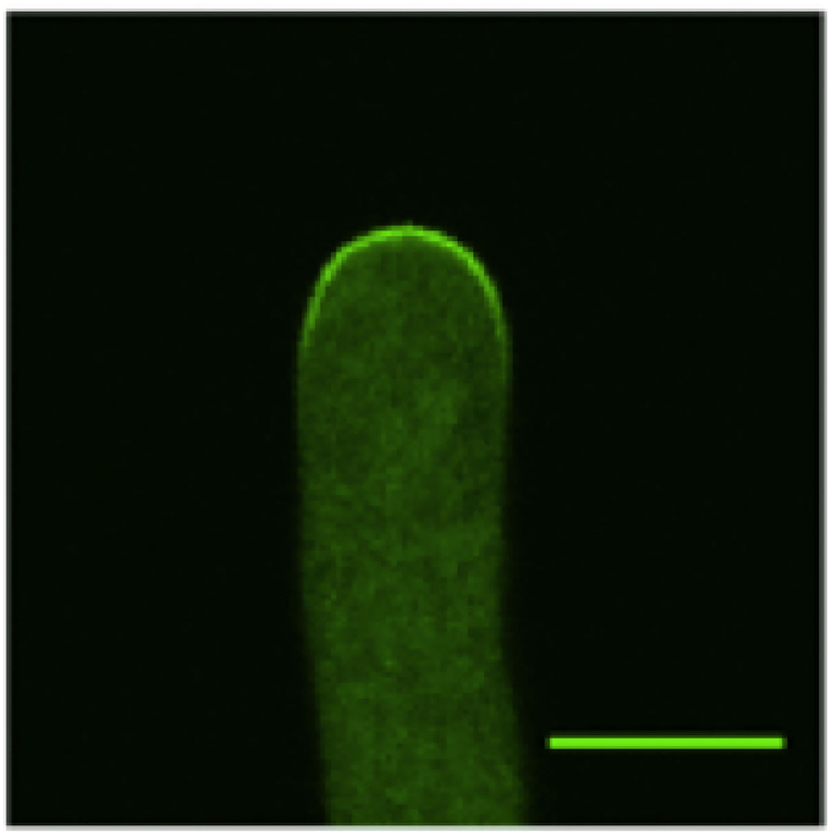
Figure 1. Confocal microscopy image of a wild-type Arabidopsis pollen tube expressing CRIB4-GFP that shows the distribution of the active ROP1. Only the tip region of the pollen tube is shown (The bar is 7 μm).
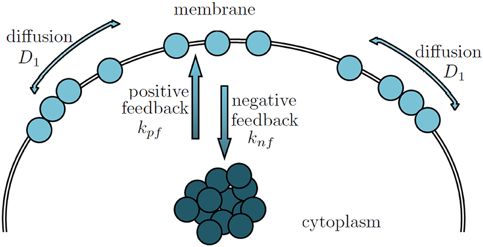
Figure 2. The formation of ROP1 polarity is determined by the positive, negative feedbacks and the lateral diffusion.
Luo et al. (2017) proposed a model of pollen tube tip growth that consists of two parts: the exocytosis-ROP1 polarization (ERP) module and the Exocytosis-Wall Extension module. In the ERP module, they proposed a system of evolutionary partial differential equation (PDE) to simulate the spatiotemporal dynamics of active ROP1 determined by the aforementioned three processes and to predict how the shape of pollen tubes changes when there is a change in positive feedback strength, negative feedback strength, or degrees of deficiency in exocytosis that regulates both positive feedback and negative feedback. Altering either one can result in pollen tubes with different widths (refer to Luo et al., 2017; Figures 1, 2 and Supplementary Figure 3). For example, a mutant with a loss of ROP1 deactivator REN1 is predicted to have an 80% reduction in negative feedback strength and therefore produces a wider tip and makes slower and smoother turnings to the guidance signal when compared to a wild type (Luo et al., 2017; Figure 1b). A weak mutant for an exocyst subunit gene SEC8 treated with 50 nM of Latrunculin B is predicted to have 43% reduction in exocytosis and therefore shows a broader distribution of active ROP1 and increased tube width when compared to a wild type. The strengths of positive and negative feedback loops in ERP module were not measurable and thus were computed using a trial-and-error method so that active ROP1 distribution can be simulated based on their evolutionary PDE model. As they pointed out, however, constructing a realistic mathematical model for pollen tube tip growth with testable and robust predictive powers requires accurately determining the strengths of positive and negative feedback loops.
Following Luo et al. (2017), we propose a similar integro-differential equation (IDE) model to describe the interplay among the aforementioned three processes that lead to ROP1 polarity formation at a steady state. Different from Luo et al. (2017), we devote our effort to estimating the strengths of positive feedback and negative feedback in the IDE model based on steady state ROP1 data. Standard parameter estimation for ordinary differential equation (ODE), such as gradient matching or generalized profiling (Ramsay et al., 2007; Brunel, 2008; Wu and Chen, 2008; Brunel et al., 2014), might be adapted to IDE under appropriate regularity assumptions (Lakshmikantham, 1995), but with challenging two identifiability issues (Miao et al., 2011). One is whether the solution of the nonlinear IDE exists and is unique (Gutenkunst et al., 2007; Transtrum et al., 2011). The other is whether the observed data are sufficient to estimate the parameters in the model (related to the Fisher Information Matrix).
Integro-differential equations of positive integer order have been widely used in many scientific areas (Bohner et al., 2021), and it is very important to investigate the qualitative properties of solutions (Tunç and Tunç, 2018). Recently, Tunç and Tunç (2018) presented sufficient and necessary conditions on the stability of the solutions to the non-linear scalar Volterra IDE and Volterra integro-differential systems of the first order. They further studied the qualitative properties of solutions to nonlinear Volterra IDE with Caputo fractional derivative, multiple kernels, and multiple constant delays and derived new sufficient conditions related to the stabilities and boundedness of solutions (Bohner et al., 2021).
Recently, there are growing applications of fractional differential equations and fractional integro differential equations in various fields such as engineering (Baleanu et al., 2020a; Bohner et al., 2021; Thabet et al., 2021) and biology (Baleanu et al., 2020c; Mohammadi et al., 2021). The Caputo and Riemann-Liouville Derivatives are the two most famous fractional derivatives that are introduced in order to take into account non-locality behavior in the phenomena of interest. The equations involved in the papers (Aydogan et al., 2018; Baleanu et al., 2019a,b, 2020a,b,c; Alizadeh et al., 2020; Matar et al., 2021; Mohammadi et al., 2021; Thabet et al., 2021) are mixed relations between integral and derivatives of the functions. While all these papers successfully addressed the critical problem of proving the existence and uniqueness of a solution to these new models, it also shows that general results for existence and uniqueness in IDE are still not found, and a careful and adapted proof should be derived on a case by case basis. The papers mentioned above use a variety of different techniques for constructing the solution: for instance, Laplace Transforms and Picard iterations.
In this paper, we exploit the closeness of our IDE to the semilinear equation, in order to apply the results of the theory of standard semilinear PDE to our case. We provide sufficient and necessary conditions for the existence and uniqueness of the solution to the proposed IDE. Furthermore, we integrate these conditions as constraints into our new Method of Moments (Lu and Meeker, 1993) estimation procedure to allow estimating positive feedback rate and negative feedback rate in a single tube IDE model or a multiple tube IDE model. For the latter case, we naturally use the framework of mixed-models (Li et al., 2002; Putter et al., 2002; Huang and Wu, 2006; Guedj et al., 2007; Lu et al., 2011) for estimating the population parameters, but we avoid the use of the likelihood. The corresponding procedure is equivalent to estimating a mixed-effects ODE model with linear constraints. We show that the estimators are consistent with asymptotic distributions under general conditions. We also prove that the two parameters are identifiable given the data.
While we could possibly incorporate fractional derivatives in our model, such modifications of our model are not necessary at this stage because we already have a very good agreement between model predictions and data. Moreover, we dedicate a large portion of the paper to measuring the population variation and the observation error, and our objective is to identify the stability of the balance between positive and negative feedbacks.
The paper is organized as follows. In Section 2, we describe how our IDE model is derived in order to characterize the distribution of active ROP1 on the membrane at a steady-state. We provide sufficient and necessary conditions for the existence and uniqueness of the solution to the proposed IDE model with a tractable and generic expression. We then introduce the IDE-based statistical models for a single pollen tube and for multiple pollen tubes. We estimate the individual and population parameters in both models, based on a constrained method of moments (CMM) procedure, and derive the asymptotic properties of CMM. We also prove that the two parameters are identifiable given the data. We examine the performance of the proposed estimation procedures through simulation studies and real data analysis in Section 3. The paper is concluded in Section 4.
2. Methods
2.1. An IDE Model for a Steady-State Distribution of Active ROP1
In this paper, we aim at deriving a mechanistic and interpretable model for distribution functions x ↦ R(x), defined on an interval [−L0, L0], where L0 ≤ +∞. The function x ↦ R(x) denotes the active ROP1 concentration at the location x on the membrane, and the function is centered such that the apical tip is obtained at the location x = 0 (as shown in Figure 3). The tube membrane is indexed by its curvilinear abscissa x, and its total length is 2 × L0. The function R is positive, bounded and the integral is equal to the quantity of ROP1 along the segment [a, b], −L0 < a < b < L0. This implies that the function R could be almost considered a non-normalized density function.
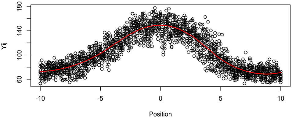
Figure 3. Imputated Data ỹij for all tubes at all locations. The red line is loess smoother.
Following the approach developed in Luo et al. (2017) and Altschuler et al. (2008), we consider a stationary PDE model that describes the equilibrium among the three competing forces that lead to ROP1 polarity formation: ROP1 activation through positive feedback with rate kpf > 0, deactivation through negative feedback with rate knf > 0, and diffusion with coefficient D1 > 0 (as shown in Figure 2). A general semilinear elliptic equation with Dirichlet conditions (Cazenave and Haraux, 1998; Badiale and Serra, 2010) can be used to describe such a stationary PDE
The rate of ROP1 lateral diffusion D1 on the plasma membrane can be measured by fluorescence recovery after photobleaching (FRAP) (Luo et al., 2017). kpf and knf are determined by ROP1-independent constants linking ROP1 activity to the local rate of exocytosis and exocytosis-independent constants determined by the enzyme activity and expression levels of GEF and GAP (Luo et al., 2017). While knf and kpf are not experimentally measurable, they can be estimated from observed active ROP1 concentration on the membrane at the steady state. Model (1) gives a direct measure of the relative importance of the different mechanisms in the system.
The functions gn and gp are positive functions that describe the laws of the underlying mechanisms. When the exact physical or chemical mechanisms are known (such as the law of mass action, or Michaelis-Menten kinetics), we can give exact functional expression. But in general, the mechanisms are often partially known and we can only consider qualitative behaviors. Typically, standard assumptions are that gn and gp are both smooth increasing functions. The linearity assumption gn(u) = u for the negative feedback is common in numerous models used in applications (Altschuler et al., 2008; Badiale and Serra, 2010; Luo et al., 2017). Remarkably, the existence and uniqueness of a positive solution (different from the trivial solution R = 0) is guaranteed under general conditions (Lions, 1982). In addition, under very general conditions on gp, this positive solution is symmetric around 0 and decreasing on [0, L0] (see Theorem 1 in Gidas et al., 1979). These results indicate that all the solutions R of the PDE models (1) share surprisingly the same qualitative properties: they are bell-shaped and even functions that vanish at the boundaries and therefore can characterize well the ROP1 distribution on the membrane as revealed in Figure 1. This typically reduces the interest in exploring the use of refined functions gp as they will provide the same pattern for R. As a consequence, we concentrate on the case of a superlinear gp, defined as , i.e., it grows faster than a linear function when u tends to infinity.
An obvious limitation of the model (1) is that the two competing positive and negative forces do not exhibit any saturation or depletion effect, as both functions gp and gn are assumed to be nondecreasing for any u > 0. For the negative feedback, it is standard to assume that the negative feedback is linear and does not depend on the actual quantity u. However, the monotonicity of the positive feedback is questionable. Indeed, the positive feedback is prone to be limited by the depletion of the available material. A standard assumption as used in the logistic equation (Murray, 2007) should be that the rate decreases with the ratio of available ROP1 in the cytosole, i.e., , where Rtot is total free ROP1 in the cell.
Putting all together, we refine the stationary PDE (1) as the following stationary IDE
Here D1 is diffusion coefficient. kpf and knf are positive feedback rate and negative feedback rate, respectively. α determines how faster the positive feedback function grows than the negative feedback function when the active ROP1 concentration goes to infinity.
Remark 1: A similar model for cell polarity was introduced in Altschuler et al. (2008), except that their model includes a spontaneous association term and α is assumed to be 1. The nonlinearity in our model comes from the product of Rα with α > 1 and the fraction of “available” ROP1 particles .
Remark 2: While the fraction plays a prominent role in a specific dynamics driven by a particular ODE in Altschuler et al. (2008), we consider directly an IDE that describes the intertwined dynamics of R and .
Remark:3 The total number of ROP1 on the membrane must be lower than the total free ROP1 Rtot in the cell, which will be an important constraint to satisfy in our model for the existence of a solution.
2.2. Identifiability of Solution R
For the reference nondimensionalized model (3) below, we can prove the existence and uniqueness of the positive solutions Uα and its limited sensitivity to α and c (see Lemma 1 in Web Appendix),
As a result, there exists unique positive solution(s) Rλ, μ(x) = λUα(μx) to the IDE (2) with and λ being the positive root(s) of the following equation
if and only if
See Proposition 1 in Web Appendix for details. Upon checking condition (5), the solution Rλ,μ(x) can be obtained as follows:
1. Solve the semilinear elliptic equation (3) on and obtain the solution Uα, compute |Uα|.
2. Compute the discriminant function Λ(·).
3. If Λ(·) = 0, compute and the unique root λ* of Equation (4) where , and compute the solution .
4. If Λ(·) < 0, compute and the positive roots and of Equation (4), and compute the solutions and . Note: In practice, the solution R closer to the experimental data will be chosen.
By solving Equation (4), we see that if Rλ,μ is a solution to the IDE (2) and Λ < 0, we have necessarily and . Consequently, with a given solution Rλ,μ, we cannot recover knf, kpf, and Rtot, because we cannot compute kpf and Rtot from a unique λ, μ. The biological implication is that we cannot recover the total free number of ROP1 in the cell by observing only ROP1 on the cell membrane. For this reason, we need to fix Rtot to be a constant. In the case of Λ = 0, we still have while is not impacted by Rtot anymore.
Let denote the fraction of active ROP1 on the membrane. The existence of positive solution Rλ,μ to IDE (2) suggests that rα−1(1 − r) ≤ (α − 1)α−1/αα, i.e., the fractions of active ROP1 on the membrane and inactive ROP1 in the cytosol at the steady state are controlled by the nonlinear growth of positive feedback force (determined by α) competing with the linear growth of the negative feedback force.
Without an integral part in IDE (2), the solutions are still of the form Rλ,μ. The parameters knf, kpf, and D1 in the equation can freely vary and the shape (height) of the solution changes with . The introduction of the saturation effect through the integral part in IDE (2) only changes the height of the peak λUα(0) (see Remark 2 in Web Appendix) with . Obviously, is an important quantity that controls the height of the peak. Recall that , the integral term implies that knf, kpf, and D1 are linked together, and that link is controlled by Rtot.
2.3. Parameter Estimation
Note that the diffusion coefficient D1 is a positive quantity that can be experimentally measured: D1 = 0.2μm (Luo et al., 2017). In order to reduce the identifiability problem between α and μ (i.e., knf, see Web Supplementary Figure 2), α is fixed at 1.2 in this paper. There is also a limited sensitivity of the solution R to α and L0 as discussed in Section 3. Furthermore, we cannot recover biologically the total free number of ROP1 (Rtot) in the cell by observing only ROP1 on the cell membrane. Adding all together, D1, α, L0, and Rtot are all assumed to be known constants and will be dropped from Λ(·) throughout this paper, and our interest lies in the estimation of the parameters kpf and knf under the constraint that the solution R of IDE (2) exists, i.e., Λ(kpf, knf) ≤ 0.
In this section, we first consider estimating knf and kpf in a constrained nonlinear fixed effect model using a single pollen tube data. We then further extend to estimate knf and kpf in a constrained nonlinear mixed effect model using multiple pollen tube data. Proposition 2 (see Web Appendix) ensures that knf and kpf can be estimated using noisy data (Miao et al., 2011) obtained either from a single pollen tube or from multiple pollen tubes.
2.3.1. Single Pollen Tube and Constrained Nonlinear Fixed Effect Model
For a single pollen tube, let Yj be the observed ROP1 intensity at a location Xj (Xj is randomly sampled from a distribution such as a uniform distribution) on the membrane at a steady state, and
where R(X; ·) is the solution of the IDE (2) and ϵj are i.i.d. random measurement errors following a certain distribution with mean 0 and variance σ2. As shown in Section 2.2, R(X; ·) exists if and only if the discriminant function Λ(knf, kpf) is non-positive. Therefore, the IDE based model (6) is subject to the following constraints
The constrained nonlinear model (6) can be reparametrized into the following model (7) with μ and λ subject to the linear constraints (8)
where and λ is the root of Equation (4). See Proposition 3 in the Web Appendix for proof. The choice of λ has been discussed in Section 2.2. We can simply estimate λ and μ first and then transpose them back to knf and kpf.
With the observations at locations obtained from the pollen tube tip growth experiment, we propose the following constrained nonlinear least square (CNLS) estimation method.
1. Compute Uα(x)
2. Estimate μ and λ by minimizing (9) under the constraints (8)
3. Convert and to and by
4. Estimate σ2 by
In step 1, Uα can be obtained by numerically solving a boundary value problem using many methods, such as the shooting method (Soetaert, 2009; Soetaert et al., 2010), the mono-implicit Runge-Kutta (MIRK) method (Cash and Mazzia, 2005), and the collocation method (Bader and Ascher, 1987) available in the R package “bvpSolve.”
To handle the linear constraint μRtot − λ|Uα| > 0 in the nonlinear least-squares minimization in the second step, we introduce a new parametrization with variable . As a result, the constrained minimization function is simplified as follows, which can be more efficiently solved by the Levenberg-Marquardt algorithm (Bertsekas et al., 1998), coded in the R package NLSR.
Among other possible choices, we propose to use the following raw estimates of the parameters as the initial values,
where ỹ0 is the closest observed value to x = 0, and δi = x(i) − x(i−1) is the step size of the sorted observations xi. Here, we exploit the fact R(0;knf, kpf) = λUα(0), and we estimate the integral directly from the data by where y(i) is the observation corresponding to x(i).
Let θ = (μ, λ)T be the parameter vector, θ0 be the true value of θ, and be the CNLS estimator with n sample measurements. For the general NLS estimator, the asymptotic properties have been established by Jennrich (1969). Wang (1996) states that the constraints have no impact on the asymptotic properties, and we have a standard normal distribution. Nevertheless, for the sake of completeness, we also consider the case when the true parameter values θ0 are on the boundary of the constrained set and give a more general result (see Proposition 4 in Web Appendix). This latter situation corresponds to the case where , i.e., all the available ROP1 is activated, and the strength of negative feedback knf is overwhelmed by a high kpf. However, this case has not been observed on real data.
2.3.2. Multiple Pollen Tube and Constrained Nonlinear Mixed Effect Model
As discussed in the introduction, our objective is to estimate at the population level the strength of the positive feedback and negative feedback processes that contribute to the ROP1 distribution and polarity formation at a steady state. In Section 3, we present data on ROP1 intensities collected from experiments on 12 different pollen tubes. For each pollen tube, we can fit the constrained nonlinear fixed effect model as described in Section 2.3.1 to the data associated with the tube and obtain the CNLS estimators. The estimated parameters are plotted in Figure 4. We can see some variability of λ and μ and a strong correlation between the two, and an even higher correlation between the original parameters knf and kpf as shown in Figure 5. For this reason, we propose to model this individual variability with a mixed model. We extend the models (6) and (7) by considering Yij, the ROP1 intensity observed for tube i at location Xij on the membrane, as follows:
where ϵij is i.i.d with mean 0 and variance σ2. We further assume that
where is a density on the constraint set , such that the mean and variance V(θi) = Σ0, for i = 1, 2, ⋯ , m. If there is no constraint, all the parameters can be estimated by several existing methods such as Ke and Wang (2001) and Wolfinger and Lin (1997). Due to the specific form of the constraint set , and the absence of “natural" assumptions on the population distribution, we only assume the existence of the first two moments: the mean θ0 and variance Σ0. The density does not need to be completely specified for population inference (typically can be a truncated Gaussian distribution on ).
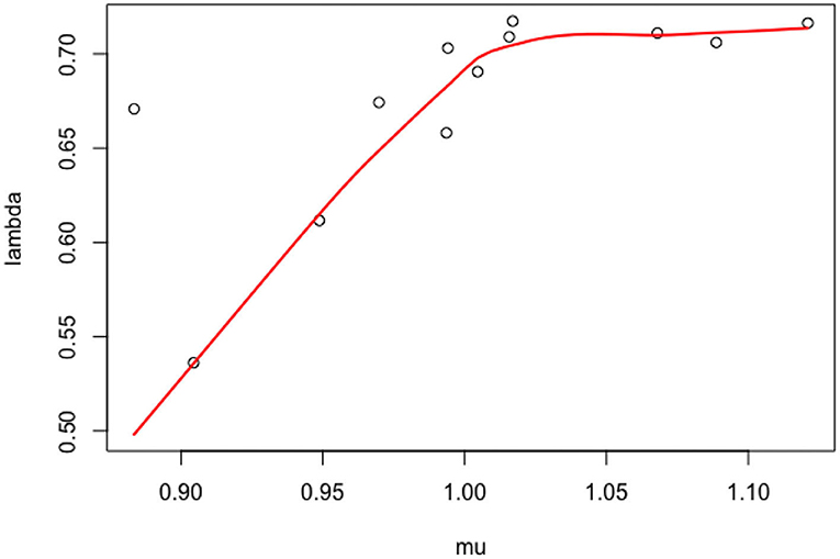
Figure 4. Scatter plot of the individual parameters (knf,i, kpf,i).
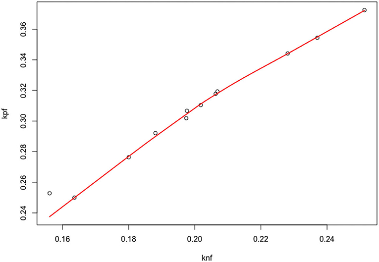
Figure 5. Scatter plot of the individual parameters (μi, λi).
Denote the experimental data to be {yij} and {xij} with i = 1, ⋯ , m and j = 1, ⋯ , ni. We assume that the mean θ0 is not on the boundary (i.e., the individual parameters θi have a null probability of being on the boundary). We first extend the CNLS procedure and propose a new procedure called CMM to estimate the nonlinear mixed effect model as follows:
1. Compute Uα(x) from Equation (3)
2. For each pollen tube i, estimate θi by minimizing least squares
under the constraints and θi > 0
3. Estimate θ0 by
4. Estimate σ2 by
5. Estimate Σ0 by , where and
6. Modify the estimator of Σ0 by
where Ψ+ is a diagonal matrix whose diagonal elements Ψii = max(ψi, 0), where ψi is the eigenvalue of , and Q is a 2 × 2 matrix whose ith columns is the eigenvector qi associated with ψi.
7. Convert to and .
This procedure is motivated by the MM proposed by Lu and Meeker (1993), and we extend it to the constrained case. The asymptotic normalities of the CMM estimators , are proved in the Web Appendix (Proposition 6).
Remark 4: If ni is sufficiently large, then the estimators θi are closed enough to the true parameters so that even with a small m, the mean (our population estimator) will be also very close to the θ0. In addition, because of the independence of the tubes, the quasi-normality of each estimator for big n implies that the population estimator will be also almost Gaussian, as a simple mean. However, if ni is not large enough, then it requires sufficiently large m to obtain a close estimate, or (approximate) Gaussianity.
We consider now the estimator of the population parameter defined as and . Let be the estimator of ϕ0. By the delta-method, we can prove the asymptotic normality of (see Corollary 2 in Web Appendix).
3. Results
3.1. Simulation Studies
In this section, our simulation studies demonstrate that the proposed methods can provide robust and accurate estimates of kpf and knf based on data from either single pollen tube or multiple pollen tubes, an important step toward a deeper understanding of the tip growth of normal and mutant pollen tubes. All the estimation procedures were implemented in R.
To evaluate the performance of the CNLS procedure, we simulated data using the values α = 1.2, D1 = 0.2, Rtot = 30, L0 = 15, knf = 0.2, and kpf = 0.3. These values were obtained empirically from real wild type Arabidopisis pollen tube data, which are also similar as those in the Supplementary Table 2 in Luo et al. (2017). Accordingly, μ = 1, λ = 0.6, and . Although our knf and kpf values are different from those used in Luo et al. (2017), our ratio of 1.5 is close to their ratio of 30 * 0.028/0.5081 = 1.65. Note that our kpf/knf is roughly equivalent to their kpf/knf × Rtot. As we mentioned earlier, it is the ratio that determines the height of the peak. The solution of Uα is solved by the collocation method (Bader and Ascher, 1987) in R package “bvpSolve.” Recall that Uα(x) is a positive and even function that achieves its maximum at x = 0. With α = 1.2, Uα(x) is close to at |x| = 5 and is close to 0 at |x| ≥ 15. Therefore, R(x) = λUα(μx) with μ = 1 in the simulation studies were generated from |x| < 15, and the range of R(x) is [0, 0.9663].
For each measurement error σ = 0.2, 0.4, we generated 10,000 data sets of size n = 51, 101, 301, i.e., x were picked along [−15, 15] with step size of 0.1, 0.3, and 0.6. CNLS based estimates of the parameters were obtained for each of the 10,000 data sets, based on which the relative bias and SD were computed as shown in Supplementary Table 1. We could see the CNLS procedure works quite well and is quite robust against noise when the size of data is fairly large. We also followed Proposition 4 to compute asymptotical variances and construct the coverage probability as shown in Supplementary Table 1. in Proposition 4 cannot be computed analytically. However, when n ≥ 300, it can be well approximated by its sample mean according to our simulation. We could see that the asymptotical variances computed based on Proposition 4 are close to those computed based on simulation, and the observed coverage appears to be approximately equivalent to the nominal confidence level.
To evaluate the performance of the CMM procedure, we generated data for each m pollen tubes with associated (μi, λi) simulate from MVN((μ, λ)T, Σ). The true values of parameters used for the simulation were knf = 0.2, kpf = 0.3, μ = 1, λ = 0.6, σ = 0.2, and Σ is a diagonal matrix with , , and .
We considered three cases. In case 1, m = 10, x is uniformly sampled from –15 to 15 with step size 0.6 and n = 51. In case 2, m = 10, x is uniformly sampled from –15 to 15 with step size 0.3 and n = 101. In case 3, m = 50, x is uniformly sampled from –15 to 15 with step size 0.1 and n = 301. Each simulation was done 10,000 times. The relative bias, SD and coverage probability for the CMM procedure are shown in Supplementary Table 2, from which we can see that the CMM procedure performs well. In particular, the asymptotical variances computed based on Proposition 6 are close to those computed based on simulation, and the observed coverage appears to be approximately equivalent to the nominal confidence level. Similar results were also observed by Yang (2001).
3.2. Pollen Tube Data Analysis
3.2.1. Data Preprocessing
In this section, we analyze data from real pollen tubes. We have measured the ROP1 intensities of 12 pollen tubes of Arabidopsis on a reference regular grid defined on (−10μm, 10μm) with a step size of 0.1205μm, therefore, m = 12 and n = 173. In order to remove outliers and to reduce excessive noise while taking into account the correlations among the 12 tubes, we replace the data with their projections on the most significant axis of a Principal Component Analysis (PCA). We select 9 axes for reconstructing the data in all the tubes (instead of 12 axes for exact reconstruction), which represent 98% of the total variance, as shown in Figure 3. Nevertheless, the tubes are not observed at all the same points xj of the reference grid, and the observed grid (xij) may vary with tube i. In order to deal with the random locations (on a common grid), we consider that the tubes have missing values (around 25% of missing values for the whole dataset) and we use the R package missMDA (Josse and Husson, 2016) for computing the axis and PCA. As a by-product of the PCA, we impute also the observations at all the locations of the reference grid, for all the tubes. For simplicity, although our mixed-effect estimator is consistent for tubes with random designs, we compute the individual and population estimators with the imputed data, so that the data are defined on the same uniform grid, for all the tubes.
As the ROP1 intensities ỹij in tubes are measured by relative intensity, it cannot represent the modeled true intensities. In particular, nonparametric smoothing estimates suggest that the functions cannot vanish at the boundaries. For this reason, we standardize the data with respect to the boundaries (where is the mean of the boundary values), in order to get ROP1 intensities that can vanish at the boundaries, as shown in Figure 6. The estimated SD of the noise is then 0.146. Figure 7 shows the normalized tubes and the smoothed estimate (in red) of Ri for i = 1, …, 12.
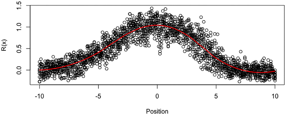
Figure 6. Normalized data yij for all tubes at all locations. Red line is loess smoother.
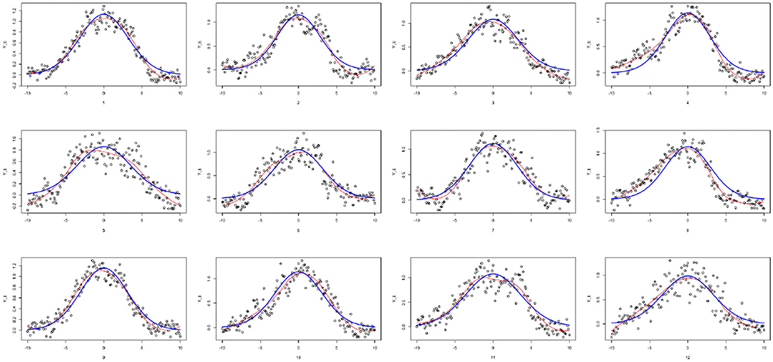
Figure 7. Individually fitted curves for each tube: loess-smoothed curves (in red), IDE solution Rλ,μ (in blue).
As the functions Ri can be written as Ri(x) = λiUα(μix), this means that any renormalization by a given constant R0 only impacts λi. If , then the normalized distribution has corresponding parameters and it satisfies the IDE
where , and the corresponding parameters are simply shifted in the following way , and the ratio is changed accordingly . This ratio is an important quantity in the IDE as it controls the height of the peak.
Note that the Equation (2) or the normalized Equation (16) are the mathematical models we construct for the ROP1 data y. The difference between its solution Ri and yij, j = 1, ⋯ , 173 for each i, i = 1, ⋯ , 12, is caused by random error as described in Equation (6) for signle pollen tube and Equation (13) for multiple pollent tube. We then apply estimation procedure detailed in Section 2.
3.2.2. Estimation of Individual Parameters
Following the results of paper (Luo et al., 2017), we assume that the diffusion parameter is D1 = 0.2, the shape parameter α = 1.2, and Rtot = 30. Moreover, as the data does not vanish exactly at the boundaries, we select L0 = 15 which permits to deal with a function that will not be exactly 0 for x = ±10. For i = 1, …, 12, we compute a rough estimate of based on the nonparametric smoother of Figure 7. We find that is between 7 and 9.5, i.e., the percentage of active ROP1 on the membrane is around 23% to 30% of Rtot. For each tube, we compute the CNLS estimates of (λi, μi) and , and σ (see Table 1). Table 1 suggests that although we have a non-negligible tube to tube variation, we can obtain pretty robust and consistent estimate for the ratio (and λ as well). This is consistent with our observation that all 12 pollen tubes have similar shapes and heights (as shown in Figure 7).
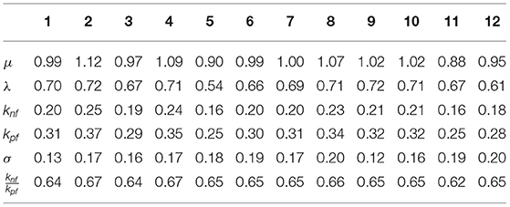
Table 1. The individual parameter estimates with constrained nonlinear least square (CNLS) for tubes i = 1, …, 12.
This suggests that estimating individual using each single pollen tube data can reveal whether the pollen tubes are undergoing the same mechanism of polarity formation or not and potentially discover new mutants with new mechanisms.
3.2.3. Estimation of the Population Parameters
If all pollen tubes are from the same population (e.g., the 12 tubes we are analyzing in this paper), we can use the constrained mixed model's approach to obtain the population parameter estimates (95% confidence interval is [0.96, 1.03]) and (95% confidence interval [0.59, 0.66]), with a SD for the noise . From these estimates, we derive the population parameter estimates for (95% Confidence Interval is [0.18, 0.21]) and (95% Confidence Interval is [0.28;0.32]).
The SD in the population are and , with an estimated correlation . The estimated correlation indicates that there is a quasi-linear relationship between knf, kpf. Above all, the mixed model permits us to estimate the correlation between the parameters and explains the strong relationship observed in Figure 5.
The multiple tube analysis and the introduction of a flexible (semi)-parametric model on the geometric properties of the densities has permitted us to infer the remarkable relationships between knf and kpf. We believe that this link is deeply related to the growth process of pollen tubes. In fact, in Luo et al. (2017), the mathematical model used shows that the tube geometry (tube width) is related to the values of the ratio , and we refer to the Web Appendix of Luo et al. (2017) in which the Figure 3a relates a given ratio to the width of pollen tubes. Our mixed-model then gives a way to measure this link through the population covariance.
4. Discussion
In this paper, we propose a statistical estimation procedure for an IDE model. Such models are quite difficult to analyze and estimate in general, as the existence of a solution and the qualitative behavior can be very specific. Nevertheless, we have shown through a mathematical analysis that the space of solutions can be reparametrized in a much more efficient manner. We have derived a versatile parametrization of the solution that links the shape of the distribution R (described with parameters μ, λ) to the competition between positive and negative feedback loops knf, kpf. Based on this relationship, we have derived an estimator with its complete statistical properties, by taking into account individual variability with a mixed model approach and asymptotic arguments. Thanks to the properties of CNLS, we can derive an estimator with few parametric assumptions on the distribution of the possible shapes of the densities Ri (we only specify the first two moments of ). Indeed, from the available data, it is arguable to assume standard parametric assumptions on , such as a Gaussian distribution—as shown in Figure 5: in our analysis, we rely instead on the asymptotic normality of the CNLS estimators. In addition, the (degenerated) deterministic relationship between knf and kpf is also very hard to introduce directly in a mixed-effects model. On the contrary, the multiple tube analysis and the introduction of a flexible (semi)-parametric model on the geometric properties of the densities has permitted to infer the remarkable relationships between knf and kpf. We think that this link is deeply related to the growth process of pollen tubes.
Oscillatory spatiotemporal Ca2+ signals have been observed in experiments, and it is identified as an important driving force of the polar cell growth in Arabidopsis pollen tubes (Luo et al., 2017). Tian et al. (2019) proposed a new reaction-diffusion model of ROP1 and Ca2+ interaction on the plasma membrane which incorporates knf,kpf, D1, and Ca2+. Estimating knf and kpf using ROP1 data at steady state proposed in this paper can provide reasonable initial values for knf and kpf in Tian et al. (2019)'s PDE model to facilitate a more complete and realistic description of the tube geometry to have better estimates, or to introduce other characteristics of the ROP1 distribution that could be related to the trade-off between negative and positive feedbacks.
The mathematical tools (in particular the theory of semilinear diffusion equation) used for deriving the existence of a solution could provide ways for deriving a tractable parametrization of the solutions set, amenable for statistical estimation. Another challenging situation is also the presence of (existence) constraints that may be reached with real data. We give in the Web Appendix the corresponding asymptotics in that situation, but the impact of reaching such constraints during estimation may have a consequence on the validity of the model and might be used for model selection. Nevertheless, in our case, the linear constraints are far from being saturated, and we always accept the NLS estimator.
Data Availability Statement
The data analyzed in this study is subject to the following licenses/restrictions: The dataset is available upon request. Requests to access these datasets should be directed to eWFuZ0B1Y3IuZWR1.
Author Contributions
XC and ZY initiated the project. ZX, NB, and XC developed the methods, theories, and wrote the paper. ZX and CT performed simulations. ZX and NB performed real data analysis. JG helped the real data analysis and interpretation. All authors contributed to the article and approved the submitted version.
Funding
This work was partially supported by the United States Department of Agriculture (USDA) National Institute of Food and Agriculture (NIFA) Hatch Project AES-CE award (CA-R-STA-7132-H) (XC) and NSF DMS 185369 (XC, ZY, and JG).
Conflict of Interest
The authors declare that the research was conducted in the absence of any commercial or financial relationships that could be construed as a potential conflict of interest.
Publisher's Note
All claims expressed in this article are solely those of the authors and do not necessarily represent those of their affiliated organizations, or those of the publisher, the editors and the reviewers. Any product that may be evaluated in this article, or claim that may be made by its manufacturer, is not guaranteed or endorsed by the publisher.
Supplementary Material
The Supplementary Material for this article can be found online at: https://www.frontiersin.org/articles/10.3389/fpls.2022.847671/full#supplementary-material
References
Alizadeh, S., Baleanu, D., and Rezapour, S. (2020). Analyzing transient response of the parallel rcl circuit by using the caputo-fabrizio fractional derivative. Adv. Diff. Equat. 2020, 55. doi: 10.1186/s13662-020-2527-0
Altschuler, S. J., Angenent, S. B., Wang, Y., and Wu, L. (2008). On the spontaneous emergence of cell polarity. Nature 454, 886–889. doi: 10.1038/nature07119
Aydogan, M., Baleanu, D., Mousalou, A., and Rezapour, S. (2018). On high order fractional integro-differential equations including the caputo-fabrizio derivative. Boundary Value Problems 2018, 90. doi: 10.1186/s13661-018-1008-9
Bader, G., and Ascher, U. (1987). A new basis implementation for a mixed order boundary value ode solver. SIAM J. Sci. Stat. Comput. 8, 483–500. doi: 10.1137/0908047
Badiale, M., and Serra, E. (2010). Semilinear Elliptic Equations for Beginners: Existence Results via the Variational Approach. London: Springer Science & Business Media.
Baleanu, D., Etemad, S., Pourrazi, S., and Rezapour, S. (2019a). On the new fractional hybrid boundary value problems with three-point integral hybrid conditions. Adv. Diff. Equat. 2019, 473. doi: 10.1186/s13662-019-2407-7
Baleanu, D., Etemad, S., and Rezapour, S. (2020a). A hybrid caputo fractional modeling for thermostat with hybrid boundary value conditions. Bound. Value Probl. 2020, 64. doi: 10.1186/s13661-020-01361-0
Baleanu, D., Etemad, S., and Rezapour, S. (2020b). On a fractional hybrid integro-differential equation with mixed hybrid integral boundary value conditions by using three operators. Alexandria Eng. J. 59, 3019–3027. doi: 10.1016/j.aej.2020.04.053
Baleanu, D., Mohammadi, H., and Rezapour, S. (2020c). Analysis of the model of hiv-1 infection of cd4+ t-cell with a new approach of fractional derivative. Adv. Diff. Equat. 2020, 71. doi: 10.1186/s13662-020-02544-w
Baleanu, D., Rezapour, S., and Saberpour, Z. (2019b). On fractional integro-differential inclusions via the extended fractional caputo-fabrizio derivation. Bound Value Probl. 2019, 79. doi: 10.1186/s13661-019-1194-0
Bassilana, M., Puerner, C., and Arkowitz, A. R. (2020). External signal - mediated polarized growth in fungi. Curr. Opin. Cell Biol. 62, 150–158. doi: 10.1016/j.ceb.2019.11.001
Bertsekas, D. P., Hager, W., and Mangasarian, O. (1998). Nonlinear Programming. Belmont, MA: Athena Scientific.
Bohner, M., Tunç, O., and Tunç, C. (2021). Qualitative analysis of caputo fractional integro-differential equations with constant delays. Comp. Appl. Math. 40, 1–17. doi: 10.1007/s40314-021-01595-3
Brunel, N. (2008). Parameter estimation of ODE's via nonparametric estimators. Electron. J. Stat. 2, 1242–1267. doi: 10.1214/07-EJS132
Brunel, N., Clairon, Q., and Dlche, F. (2014). Parametric estimation of ordinary differential equations with orthogonality conditions. J. Am. Stat. Assoc. 109, 173–185. doi: 10.1080/01621459.2013.841583
Campas, O., and Mahadevan, L. (2009). Shape and dynamics of tip-growing cells. Curr. Biol. 19, 2102–2107. doi: 10.1016/j.cub.2009.10.075
Cash, J., and Mazzia, F. (2005). A new mesh selection algorithm, based on conditioning, for two-point boundary value codes. J. Comput. Appl. Math. 184, 362–381. doi: 10.1016/j.cam.2005.01.016
Cazenave, T., and Haraux, A. (1998). An Introduction to Semilinear Evolution Equations, Volume 13 of Oxford Lecture Series in Mathematics and Its Applications. New York, NY: The Clarendon Press Oxford University Press.
Dumais, J., Shaw, S., Steele, C., Long, S., and Ray, P. (2006). An anisotropic-viscoplastic model of plant cell morphogenesis by tip growth. Int. J. Dev. Biol. 50, 209–222. doi: 10.1387/ijdb.052066jd
Fayant, P., Girlanda, O., Chebli, Y., Aubin, C., Villemure, I., and Geitmann, A. (2010). Finite element model of polar growth in pollen tubes. Plant Cell. 22, 2579–2593. doi: 10.1105/tpc.110.075754
Gidas, B., Ni, W., and Nirenberg, L. (1979). Symmetry and related properties via the maximum principle. Commun. Math. Phys. 68, 209–243. doi: 10.1007/BF01221125
Gow, N. (1994). Growth and guidance of the fungal hypha. Microbiology 140, 3193–3205. doi: 10.1099/13500872-140-12-3193
Gow, N. A., Brown, A. J. P., and Odds, F. C. (2002). Fungal morphogenesis and host invasion. Curr. Opin. Microbiol. 5, 366–371. doi: 10.1016/S1369-5274(02)00338-7
Gu, Y., Vernoud, V., Fu, Y., and Yang, Z. (2003). Rop gtpase regulation of pollen tube growth through the dynamics of tip-localized f-actin. J. Exp. Bot. 54, 93–101. doi: 10.1093/jxb/erg035
Guedj, J., Thiebaut, R., and Commenges, D. (2007). Maximum likelihood estimation in dynamical models of hiv. Biometrics 63, 1198–1206. doi: 10.1111/j.1541-0420.2007.00812.x
Guo, J., and Yang, Z. (2020). Exocytosis and endocytosis: coordinating and fine-tuning the polar tip growth domain in pollen tubes. J. Exp. Bot. 71, 2428–2438. doi: 10.1093/jxb/eraa134
Gutenkunst, R. N., Waterfall, J. J., Casey, F. P., Brown, K. S., Myers, C. R., and Sethna, J. P. (2007). Universally sloppy parameter sensitivities in systems biology models. PLoS Comput. Biol. 3, e189. doi: 10.1371/journal.pcbi.0030189
Hepler, P., Vidali, L., and Cheung, A. (2001). Polarized cell growth in higher plants. Annu. Rev. Cell Dev. Biol. 17, 159–187. doi: 10.1146/annurev.cellbio.17.1.159
Huang, Y., and Wu, H. (2006). A bayesian approach for estimating antiviral efficacy in hiv dynamic models. J. Appl. Stat. 33, 155–174. doi: 10.1080/02664760500250552
Hwang, J., Wu, G., Yan, A., Lee, Y., Grierson, C., and Yang, Z. (2010). Pollen-tube tip growth requires a balance of lateral propagation and global inhibition of rho-family gtpase activity. J. Cell Sci. 123, 340–350. doi: 10.1242/jcs.039180
Jennrich, R. I. (1969). Asymptotic properties of non-linear least squares estimators. Ann. Math. Stat. 40, 633–643. doi: 10.1214/aoms/1177697731
Josse, J., and Husson, F. (2016). Missmda: a package for handling missing values in multivariate data analysis. J. Stat. Softw. 70, 1–31. doi: 10.18637/jss.v070.i01
Ke, C., and Wang, Y. (2001). Semiparametric nonlinear mixed-effects models and their applications. J. Am. Stat. Assoc. 96, 1272–1298. doi: 10.1198/016214501753381913
Kroeger, J. H., Geitmann, A., and Grant, M. (2008). Model for calcium dependent oscillatory growth in pollen tubes. J. Theor. Biol. 253, 363–374. doi: 10.1016/j.jtbi.2008.02.042
Lee, Y., and Yang, Z. (2008). Tip growth: Signaling in the apical dome. Curr. Opin. Plant Biol. 11, 662–671. doi: 10.1016/j.pbi.2008.10.002
Li, H., Wu, G., Ware, D., Davis, K., and Yang, Z. (1998). Arabidopsis rho-related gtpases: differential gene expression in pollen and polar localization in fission yeast. Plant Physiol. 118, 407–417. doi: 10.1104/pp.118.2.407
Li, L., Brown, M., Lee, K., and Gupta, S. (2002). Estimation and inference for a spline-enhanced population pharmacokinetic model. Biometrics 58, 601–611. doi: 10.1111/j.0006-341X.2002.00601.x
Lin, Y., Wang, Y., Zhu, J., and Yang, Z. (1996). Localization of a rho gtpase implies a role in tip growth and movement of the generative cell in pollen tubes. Plant Cell 8, 293–303. doi: 10.2307/3870272
Lions, P. L. (1982). On the existence of positive solutions of semilinear elliptic equations. SIAM Rev. 24, 441–467. doi: 10.1137/1024101
Lowery, L., and Vanvactor, D. (2009). The trip of the tip: understanding the growth cone machinery. Nat. Rev. Mol. Cell Biol. 10, 332–343. doi: 10.1038/nrm2679
Lu, C. J., and Meeker, W. Q. (1993). Using degradation measures to estimate a time-to-failure distribution. Technometrics 35, 161–174. doi: 10.1080/00401706.1993.10485038
Lu, T., Liang, H., Li, H., and Wu, H. (2011). High dimensional odes coupled with mixed-effects modeling techniques for dynamic gene regulatory network identification. J. Am. Stat. Assoc. 106, 1242–1258. doi: 10.1198/jasa.2011.ap10194
Luo, N., Yan, A., Liu, G., Guo, J., Rong, D., Kanaoka, M., et al. (2017). Exocytosis-coordinated mechanisms for tip growth underlie pollen tube growth guidance. Nat. Commun. 8, 1687. doi: 10.1038/s41467-017-01452-0
Matar, M., Abbas, M., Alzabut, J., Kaabar, M., Eternad, S., and Rezapour, S. (2021). Investigation of the p-laplacian nonperiodic nonlinear boundary value problem via generalized caputo fractional derivatives. Adv. Diff. Equat. 2021, 68. doi: 10.1186/s13662-021-03228-9
Miao, H., Xia, X., Perelson, A., and Wu, H. (2011). On identifiability of nonlinear ode models with application in viral dynamics. SIAM Rev. 53, 3–39. doi: 10.1137/090757009
Mohammadi, H., Kumar, S., Rezapour, S., and Etemad, S. (2021). A theoretical study of the caputo—fabrizio fractional modeling for hearing loss due to mumps virus with optimal control. Chaos Solitons Fractals 144, 110668. doi: 10.1016/j.chaos.2021.110668
Murray, J. D. (2007). Mathematical Biology: I. An introduction, volume 17. New York, NY: Springer Science & Business Media.
Palanivelu, R., and Preuss, D. (2000). Pollen tube targeting and axon guidance: parallels in tip growth mechanisms. Trends Cell Biol. 10, 517–524. doi: 10.1016/S0962-8924(00)01849-3
Putter, S. H., Heisterkamp, J. M. A. L., and de Wolf, F. (2002). A bayesian approach to parameter estimation in hiv dynamical models. Stat. Med. 21, 2199–2214. doi: 10.1002/sim.1211
Qin, Y., and Yang, Z. (2011). Rapid tip growth: insights from pollen tubes. Sem. Cell Dev. Biol. 22, 816–824. doi: 10.1016/j.semcdb.2011.06.004
Ramsay, J. O., Hooker, G., Campbell, D., and Cao, J. (2007). Parameter estimation for differential equations: a generalized smoothing approach. J. R. Stat. Soc. B 69, 741–796. doi: 10.1111/j.1467-9868.2007.00610.x
Soetaert, K. (2009). rootSolve: Nonlinear root finding, equilibrium and steady-state analysis of ordinary differential equations. R package 1.6.
Soetaert, K., Petzoldt, T., and Setzer, R. W. (2010). Solving differential equations in r: Package desolve. J. Stat. Softw. 33, 1–25. doi: 10.18637/jss.v033.i09
Takano, T., Funahashi, Y., and Kaibuchi, K. (2019). Neuronal polarity - positive and negative feedback signals. Front. Cell Dev. Biol. 7, 69. doi: 10.3389/fcell.2019.00069
Thabet, S., Etemad, S., and Rezapour, S. (2021). On a coupled caputo conformable system of pantograph problems. Turkish J. Math. 2021, 496–519. doi: 10.3906/mat-2010-70
Tian, C., Shi, Q., Cui, X., Guo, J., Yang, Z., and Shi, J. (2019). Spatiotemporal dynamics of a reaction-diffusion model of pollen tube tip growth. J. Math. Biol. 79, 1319–1355. doi: 10.1007/s00285-019-01396-7
Transtrum, M. K., Machta, B. B., and Sethna, J. P. (2011). Geometry of nonlinear least squares with applications to sloppy models and optimization. Phys. Rev. E 83, 036701. doi: 10.1103/PhysRevE.83.036701
Tunç, C., and Tunç, O. (2018). New qualitative criteria for solutions of volterra integro-differential equations. Arab J. Basic Appl. Sci. 25, 158–165. doi: 10.1080/25765299.2018.1509554
Wang, J. (1996). Asymptotics of least-squares estimators for constrained nonlinear regression. Ann. Stat. 24, 1316–1326. doi: 10.1214/aos/1032526971
Wen, Z., and Zheng, J.-Q. (2006). Directional guidance of nerve growth cones. Curr. Opin. Neurobiol. 16, 52–58. doi: 10.1016/j.conb.2005.12.005
Wolfinger, R., and Lin, X. (1997). Two taylor-series approximation methods for nonlinear mixed models. Comput. Stat. Data Anal. 25, 465–490. doi: 10.1016/S0167-9473(97)00012-1
Wu, H., and Chen, J. (2008). Estimation of time-varying parameters in deterministic dynamic models. J. Am. Stat. Assoc. 103, 369–384. doi: 10.1198/016214507000001382
Yang, M. A.-Z. S. (2001). An approximate em algorithm for nonlinear mixed effects models. Biometr. J. 43, 881–893. doi: 10.1002/1521-4036(200111)43:7<881::AID-BIMJ881>3.0.CO;2-S
Yang, Z. (1998). Signaling tip growth in plants. Curr. Opin. Plant Biol. 1, 523–530. doi: 10.1016/S1369-5266(98)80046-0
Keywords: cell polarity, constrained semiparametric regression, identifiability, integro-differential equation, method of moments, semilinear elliptic equation
Citation: Xiao Z, Brunel N, Tian C, Guo J, Yang Z and Cui X (2022) Constrained Nonlinear and Mixed Effects Integral Differential Equation Models for Dynamic Cell Polarity Signaling. Front. Plant Sci. 13:847671. doi: 10.3389/fpls.2022.847671
Received: 18 January 2022; Accepted: 08 April 2022;
Published: 25 May 2022.
Edited by:
Ingo Dreyer, University of Talca, ChileReviewed by:
Cemil Tunç, Yznc Yıl University, TurkeyShahram Rezapour, Azarbaijan Shahid Madani University, Iran
Copyright © 2022 Xiao, Brunel, Tian, Guo, Yang and Cui. This is an open-access article distributed under the terms of the Creative Commons Attribution License (CC BY). The use, distribution or reproduction in other forums is permitted, provided the original author(s) and the copyright owner(s) are credited and that the original publication in this journal is cited, in accordance with accepted academic practice. No use, distribution or reproduction is permitted which does not comply with these terms.
*Correspondence: Xinping Cui, eHBjdWlAdWNyLmVkdQ==