Methane dynamics from a mixed plantation of north China: Observation using closed-path eddy covariance method

Although an important greenhouse gas, methane flux in hilly forest ecosystems remains unclear. By using closed-path eddy covariance systems, methane flux was measured continuously from 2017 to 2019 in a mixed plantation in the Xiaolangdi area of the Yellow River in North China. The methane flux footprint and its diurnal and monthly variations were analysed, and its characteristics on rainy days are discussed. The results showed that: (a) the observation data were reliable with good spatial representation (b) The methane flux in the mixed plantation ecosystem had obvious diurnal and seasonal variations: the monthly average diurnal variation of the methane flux had a single-peak; the methane flux value was source in the daytime and sink at night. The daily mean maximum value of methane flux in growing season was lower than that in non-growing season with the maximum value appearing in March, and the minimum value in October. (c) The forest is an atmospheric CH₄ source with the annual emission in 2017 of (3.31 g C·m^-2·year ^-1) >2019 (2.94 g C·m^-2·year^-1) >2018 (2.81 g C·m^-2·year ^-1), and the main influencing factor was precipitation. Rainfall affected CH₄ flux with a lag period of approximately three days. Rainfall also changed the balance of CH₄ flux between sink or source according to precipitation intensity and frequency.

1 Introduction

CH₄ is the third largest greenhouse gas after water vapour and CO₂, but its greenhouse effect over 100 years is 28 times that of CO₂ (IPCC, 2013). On the global scale, approximately 10 Tg·a^-1 of CH₄ emissions are from unexplained sources (Megonigal and Guenther, 2008). The attribution of these emissions to particular sources and sinks is still an unresolved issue for the scientific community. Forest ecosystems cover most continental regions, and any sink-to-source transitions could have a non-negligible impact on global atmospheric CH₄ budgets. Therefore, it is important to understand CH₄ dynamics in forest ecosystems and CH₄ exchange between the atmosphere and forests.

Considering that a major portion of forest soil is water-unsaturated, forests are generally assumed to be an insignificant atmospheric CH₄ sink, representing about 6% of the global sink (Machacova et al, 2016). However, studies have revealed that forest ecosystems are not always CH₄ sinks. Some global inversions of CH₄ have indicated that broadleaf evergreen forests and tropical forests might be important CH₄ sources (Frankenberg et al., 2005), contrary to the traditional view that forests always absorb atmospheric CH₄. These results suggest that CH₄ originates from a wider range of sources than previously considered. All biological surfaces in a forest, including living and dead wood, can exchange CH₄, usually emitting CH₄ (Covey and Megonigal, 2018; Pitz and Megonigal, 2017), indicative of a reduced sink and even a CH₄ source in forest ecosystems. It is important to quantify CH₄ fluxes in forest ecosystems (Shoemaker et al., 2014; Ueyama et al., 2018).

Ecosystem scale CH₄ sources and sinks are uncertain in different forests. Smeets et al. (2009) revealed the Ponderosa pine forest ecosystem was a CH₄ sink, while Miyama et al. (2010) had observed no CH₄ flux changes from an oak-holly mixed forest in the warm temperate zone. Spatial heterogeneity of CH₄ sources and sinks exist in the forest ecosystem, and while the forest is a CH₄ source at the canopy scale, the forest ground surface absorbs CH₄ (Simpson et al., 1999; Miyama et al., 2010; Mikkelsen et al., 2012; CoveyMegonigal, 2018; Nakai et al., 2020). The diurnal dynamic reflects a CH₄ sink at the annual scale and in the growth season but indicates a CH₄ sink during daytime and in the non-growth season (Ueyama et al., 2013; Sundqvist et al., 2015; Gao et al., 2016). Consequently, the underlying surface is complex due to diverse climates and forest types, consequently the aforementioned studies lack generalizability. In contrast to CO₂ fluxes, there are relatively few studies on CH₄ fluxes in forest ecosystems, and the published papers usually have relatively short durations of observation and data collection, making it impossible to evaluate and predict the global forest CH₄ budget accurately, and the source-sink transition pattern and its role in the CH₄ cycle are still not well understood.

Eddy covariance technology provides a reliable approach to measuring the CH₄ fluxes. This study focuses on the methane flux dynamics at daily, seasonal, and interannual time scales based on 3 years (2017–2019) of eddy covariance flux observation in a mixed plantation of north China. The specific objectives of this study are to (1) identify CH₄ dynamics at different time scales, and (2) clarify CH₄ changes during the rainy days and provide a scientific foundation for accurately estimating CH₄ fluxes.

2 Materials and methods

2.1 Site description

This experiment was conducted at the Xiaolangdi forest research station, Chinese Academy of Forestry Sciences. The station is located at Jiyuan County, Henan, China (35°01′ N, 112°28′ E; elevation 410 m), south of Taihang mountain and north of the Yellow River Basin. It has a warm-temperate continental monsoon climate. The average annual air temperature was 13.4°C. The annual mean rainfall was 642 mm, with an average growing season (April–October) rainfall of approximately 438 mm, making up approximately 60% of the whole year. The average annual sunshine hours are 2377.7 h. The stand is dominated by cork oak (Quercus variabilis Blume), which was planted in 1973, with a mean height of 10.5 m. The other trees include black locust (Robinia pseudoacacia L.) and arborvitae (Platycladus orientalis), with ages of 28 and 30 years and heights of 9.3 m and 8.2 m, respectively. The planting density was 1905 stems ha^-1, and the stand coverage was 96%. The understory is sparse and mainly composed of sour jujube [Ziziphus jujuba Mill. var. inermis (Bunge) Rehd.], Bunge’s hackberry (Celtis bungeana BI), and green bristlegrass [Setaria viridis (L.) Beauv.]. The soil was principally brown loam, with an average thickness of 0.4 m. The flux observation tower (36 m) is situated at the centre of a large plantation area (7210 ha). The mean LAI of the mixed plantation is 6.3 during the growing season. The mean slope around the flux observation tower is 14° (Tong et al., 2012).

2.2 Methane flux and microclimate measurements

The closed-path eddy covariance (CPEC) system consists of a 3-D sonic anemometer (Model CSAT3; Campbell Scientific), a closed-path fast greenhouse gas analyser (FGGA; Los Gatos Research, Mountain View, CA, USA) and a dry vacuum scroll pump (XDS35i; BOC Edwards, Crawley, UK), requiring 520 W of power. All instruments were installed at a height of 30 m. Raw data were collected at 10 Hz and recorded by a CR5000 datalogger (Campbell Scientific).

In the CPEC system, an inlet tube situated at the same height as the anemometer, with a separation of 15 cm, was used to draw air into the FGGA. This analyser measures CH₄, CO₂ and H₂O concentrations by off-axis integrated cavity ringdown spectroscopy (Baer et al., 2002). During the experiment, the pump drew the sample air through a 40-m tube (inner diameter: 5 mm) at flow rates of about 40 L min⁻¹ into the measuring cell under an operating pressure of approximately 19 kPa. The air passed through an initial filter with a pore size of 100 μm to prevent dust and insects from entering the system, as well as through 5 μm and 2 μm external plum sharp filters at the end of the tube, and finally through two 2 μm metal filters (one internal and one external) before entering the measuring cell. The 100 μm filter is replaced every 6 months, while the external plum sharp filters and porous filters are replaced every 3 months to maintain clean optics and avoid inflow restrictions. Because the pump and the gas analyser have a high power requirement, the CPEC system ran on AC power during the measurement period.

2.3 Data processing

Processing of the raw EC data was performed using EddyPro 6.2 (LI-COR; available at www.licor.com/eddypro ). De-spiking and absolute limit determinations were included in the preliminary processing of raw signals (Vickers and Mahrt, 1997). At this preliminary stage, outliers also were discarded. This involves filtering for spikes and linear detrending. Double coordinate rotations were performed to align the mean vertical velocity measurements normal to the mean wind streamlines before carrying out scalar flux calculations (Wilczak et al., 2001). Using the covariance maximisation method (relative to the vertical velocity of temperature), the time lag was determined for each 30-min period. Half-hourly fluxes of CH₄ were calculated as the mean covariance of vertical wind velocity and scalar fluctuations in CH₄ concentrations. The Webb–Pearman–Leuning correction for density fluctuations arising from variations in water vapour was applied as described in Ibrom et al. (2007b). Low-pass filtering effects were assessed and corrected using the method of Ibrom et al. (2007a), based on in situ determination of water vapour attenuation and a model for the corresponding spectral correction factor. Quality control criteria according to Mauder and Foken (2004) were used to reject abnormal data. In addition, data were excluded when the pump stopped working, during maintenance or high temperature in summer, or when the sonic anemometer signal was degraded during heavy rain. The data from June to September in 2017 were used to determine the friction velocity (u*) threshold using R package ‘REddyProc’ (https://github.com/bgctw/REddyProc ). The average flux increased along with u* until it tended to level off and be independent of u* at around 0.1 m s^-1. Data collected during weak turbulence were removed from analyses by filtering out all half-hourly flux measurements with a friction velocity (u*) below 0.1 m s^-1. Time delays were calculated through the use of a cross-correlation function of the scalar fluctuation and the vertical wind velocity. The lag time was set as 8 s by comparing with an open-path eddy covariance system (Yuan et al., 2019). Atmospheric stability has a direct impact on the distribution of flux footprint, which is subsequently affected by wind speed, atmospheric temperature, and properties of the underlying surface. Therefore, the atmosphere was divided into stable state (Zm/L>0) and unstable state (Zm<0) according to the atmospheric stability Zm/L, where Zm is the height observed by instrument and L is the Obukhov length. The footprint model was used to analyse the source distribution of the flux signal. The data separated by more than three times the variance from the average were regarded as abnormal. Moreover, abnormal data reflecting instrument malfunction or unfavourable meteorological conditions (rain and dew) were also eliminated. A linear method was used to fill the gaps when data were missing, within 2 h. The larger gaps in the daytime and night-time were filled using the mean diurnal variation (MDV) and nonlinear regression methods, respectively (Falge et al., 2001). The finial calculation of CH₄ fluxes value is positive which represent the methane source, and the value is negative with methane sink.

3 Result

3.1. Characteristics of CH₄ flux footprint in Ecosystem

In this study, the eddy covariance flux data between 2017 and 2019 were analysed. A contour map of the flux footprint was drawn using Footprint software, taking the 90% flux footprint as the measurement target. The area was calculated by the grid area method and was used to analyse the changes of CH₄ flux footprint.

Analyses of the wind direction and speed data between 2017 and 2019 showed that the measurement area experienced easterly wind (at 90°) and west-south-westerly wind (between 225° and 270°) (Figure 1). This is consistent with the measurements obtained from previous years, which showed that winds in this area were predominantly east-north-easterly and west-south-westerly (Zheng et al, 2010). The maximum wind speeds in 2017, 2018, and 2019 were respectively 10.8 m·s^-1, 12.3 m·s^-1, and 10.6 m·s^-1, while the average wind speeds were respectively 3.2 m·s^-1, 3.2 m·s^-1, and 3.1 m·s^-1.

FIGURE 1

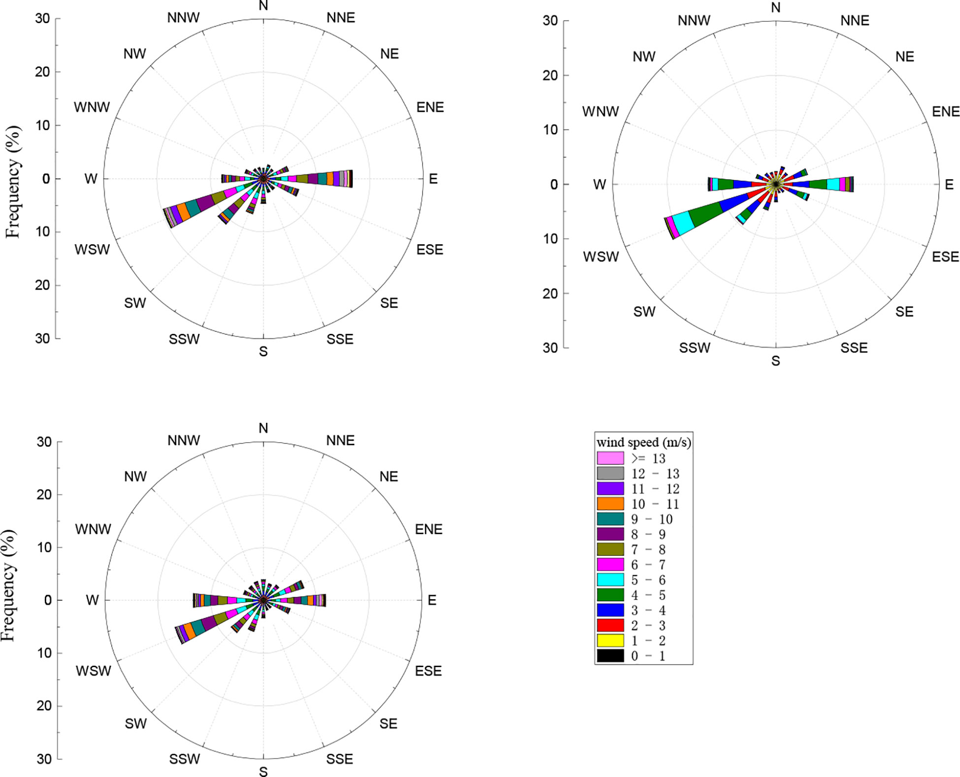
Figure 1 2017–2019 wind roses.

Figure 2 shows the flux footprint under different conditions of atmospheric stability during the growth (August) and non-growth seasons (December) in 2017. The footprint was taken 80% as the target, regardless of season (growth or non-growth), the footprint was consistently smaller without atmospheric stability, owing to the intense material exchange between canopy and atmosphere when the atmosphere is unstable. In addition, flux information captured by the sensor mainly came from upwind of the sensor. Moreover, the footprint was smaller during the growth season because the flux measurements were from the underlying surface further to windward of the sensor, as the leaf area index is greater during the growth season and is influenced by the underlying surface.

FIGURE 2

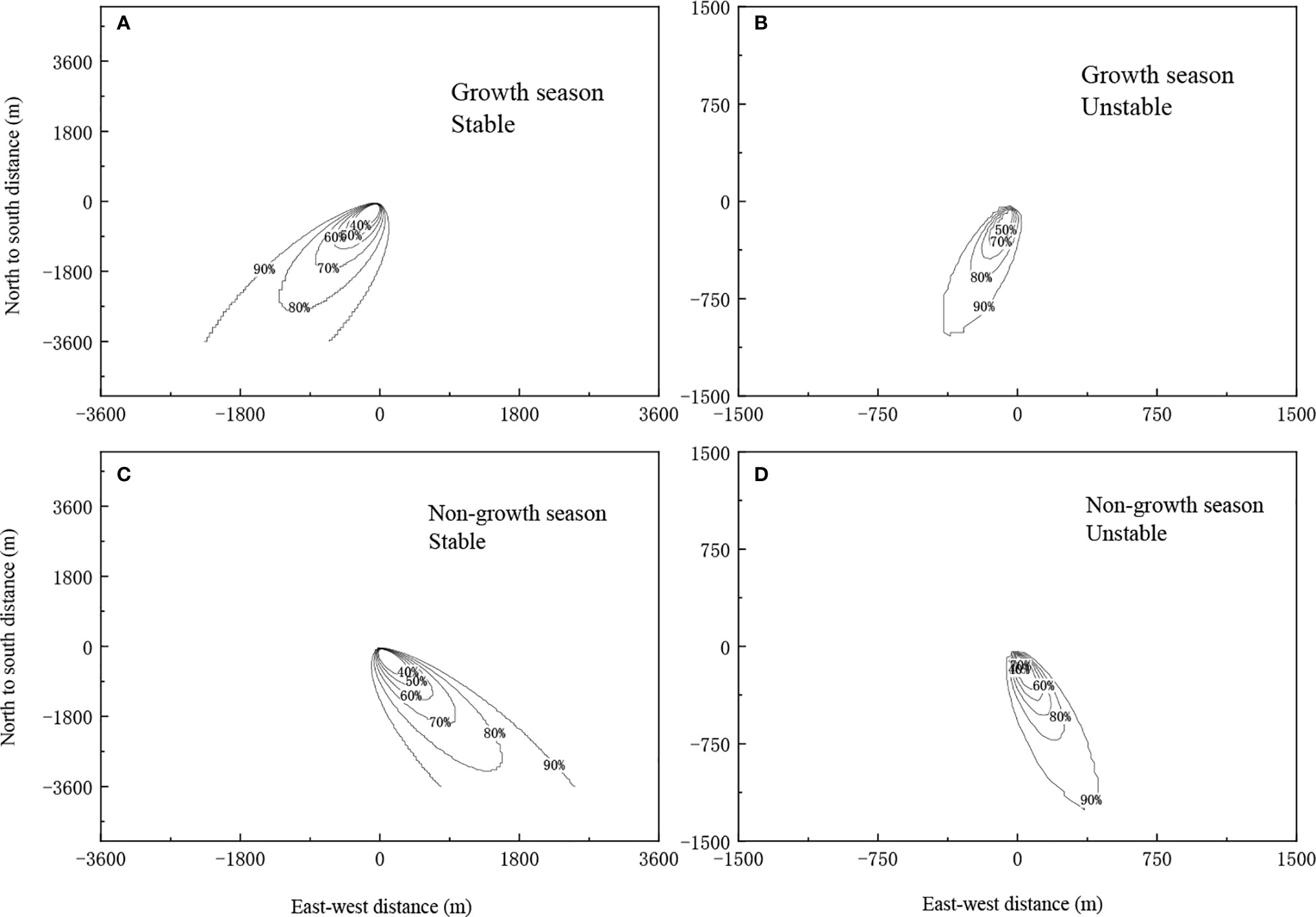
Figure 2 The footprint under different stability conditions during the growth and non-growth seasons of 2017.(A) Growth season, Stable. (B) Growth season, Unstable. (C) Non-growth season, Stable. (D) Non-growth season, Unstable.

The flux footprint throughout August 8^th, 2017, which was a typical sunny day, was analysed taking 3 h as the time interval. The distribution was non-uniform, and the flux changes throughout the day can be easily observed in Figure 3. At 3:00, the flux footprint was approximately 3000 m east to west and 600 m north to south, accounting for an area of 1.26 km²; at 9:00, the flux footprint was approximately 2520 m east to west and 720 m north to south, accounting for an area of 1.04 km²; at 15:00, the flux footprint was approximately 600 m east to west and 150 m north to south, accounting for an area of 0.06 km²; and at 21:00 was approximately 1300 m east to west and 900 m north to south, accounting for an area of 0.28 km². Throughout the day, the flux footprint was in general consistently distributed to windward. In summary, the eddy covariance measurement system measures the size of the windward flux footprint, and the data represented the flux of the study area well.

FIGURE 3

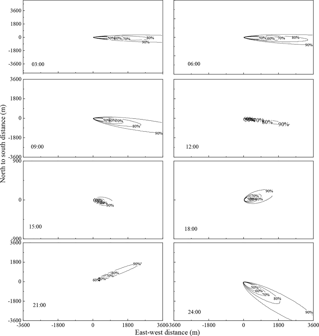
Figure 3 Changes in flux footprint over time within a typical sunny day (August 8^th, 2017).

3.2 Characteristics of CH₄ flux changes with time in ecosystem

3.2.1 Daily change in CH₄ flux

3.2.1.1 Diurnal variation in CH₄ flux averaged by month

The CH₄ flux in the ecosystem showed obvious changes throughout a day (Figure 4). For each month, the average within-day changes in CH₄ flux followed an inverted U-shape pattern: CH₄ flux changed from negative to positive after sunrise due to the increase in radiation and temperature, and the ecosystem served as a CH₄ source in the atmosphere, the CH₄ flux reached its maximum value at 15:00, after which it decreased gradually as the radiation and temperature decreased. The CH₄ flux became negative around sunset, causing the ecosystem to become a CH₄ sink for the atmosphere. The CH₄ flux remained unchanged during the night, due to the influence of weak turbulence.

FIGURE 4

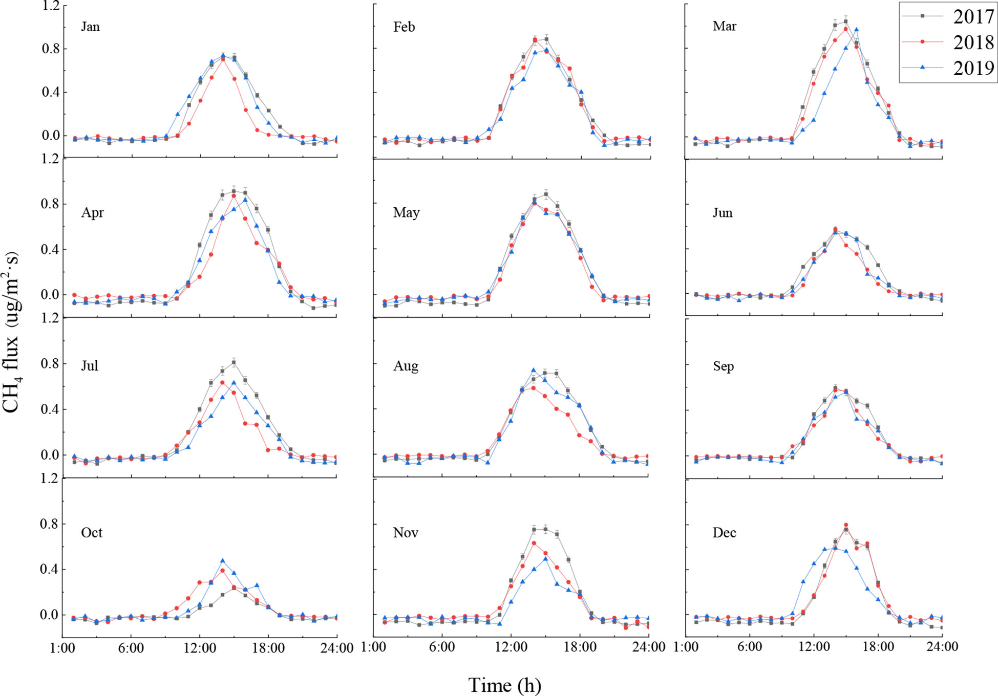
Figure 4 Average within-day CH₄ flux of the ecosystem by month. Error bars show standard deviation.

The CH₄ flux of the ecosystem showed similar obvious within-day changes across months, with some months showing slightly different changes (Figure 4). The average within-day CH₄ flux was highest in March, reaching 1.11 μg·m^-2·s^-1, 0.97 μg·m^-2·s^-1, and 0.99 μg·m^-2·s^-1 respectively in 2017, 2018, and 2019. The average within-day CH₄ flux was lowest in October, reaching 0.26 μg·m^-2·s^-1, 0.42 μg·m^-2·s^-1, and 0.48 μg·m^-2·s^-1 respectively in 2017, 2018, and 2019, which differed markedly from the CH₄ flux in March. The CH₄ flux changed from negative to positive at the earliest in July (at around 8:30) and at the latest in November (at around 10:00). The CH₄ flux changed from positive to negative around July to August at the latest (at around 19:30), and this change gradually became earlier from September until it reached its earliest around 18:00 in December. As a result, the CH₄ flux remained positive for the longest period in July (11 h), and the shortest period in October (8 h) (Figure 4). Radiation and temperature reached their maximum values around June each year in the current study area, yet the CH₄ flux (both daily maximum and daily average) of the ecosystem was less than in adjacent months, owing to the high temperature and small precipitation in June.

The CH₄ flux of the ecosystem during the growth and non-growth seasons during the study period was positive during the day and did not change much during the night (Figure 5). During the growth season, the CH₄ flux increased rapidly from 10:00 to 14:00, and decreased slowly from 14:00 to 20:00. During the non-growth season, the CH₄ flux also increased rapidly from 10:00 to 14:00 and to a higher peak, and decreased from 14:00 to 20:00 (Figure 5). This is consistent with the results reported by Tong et al. (2012) on the CO₂ flux of the same ecosystem. This can be explained by the relatively high temperature in the afternoon in spring and summer, causing VPD to be relatively large.

FIGURE 5

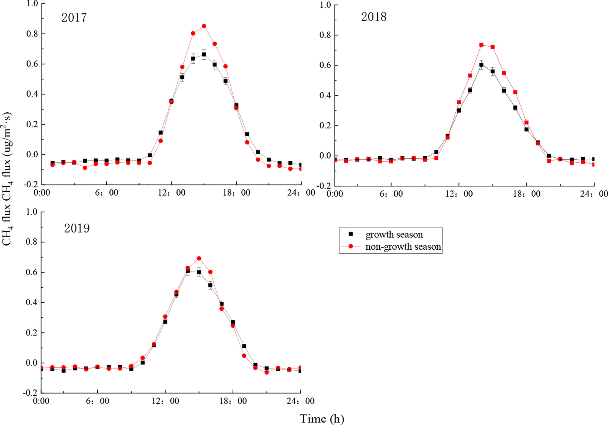
Figure 5 Changes in average within-day CH₄ flux by month during the growth and non-growth seasons. Error bars show standard deviation.

The daily maximum of CH₄ flux was lower during the growth season than during the non-growth season (Figure 5), mainly because precipitation is high during the growth season. As the growth season transitions into the non-growth season (November to March), radiation and temperature gradually decrease, and the forest soil serves as a CH₄ source as most trees, except for coniferous species such as Platycladus orientalis, experience withering and leaf fall (Zhuang et al, 2016). Therefore, CH₄ flux is lower in the growth season.

3.2.1.2 Diurnal variation of CH₄ flux on sunny and rainy days

Typical sunny days (April 27^th, 2017; December 6^th, 2017; February 22^nd, 2018; September 7^th, 2018; May 22^nd, 2019; November 14^th, 2019) and rainy days (May 22^nd, 2017; November 28^th, 2017; February 18^th, 2018; August 20^th, 2018; May 29^th, 2019; November 12^th, 2019) in the growth and non-growth seasons were selected to analyse the within-day changes in the CH₄ flux of the ecosystem. These CH₄ fluxes all followed an inverted U-shape pattern, where the CH₄ flux was positive during the day and showed significant changes, and the changes were more complicated on rainy days (Figure 6). On a sunny day, as radiation and temperature increased after sunrise, CH₄ flux also gradually increased until reaching its maximum value around 13:30. In contrast, when the atmosphere was relatively stable during the night and the air turbulence was weak, CH₄ flux showed no significant changes.

FIGURE 6

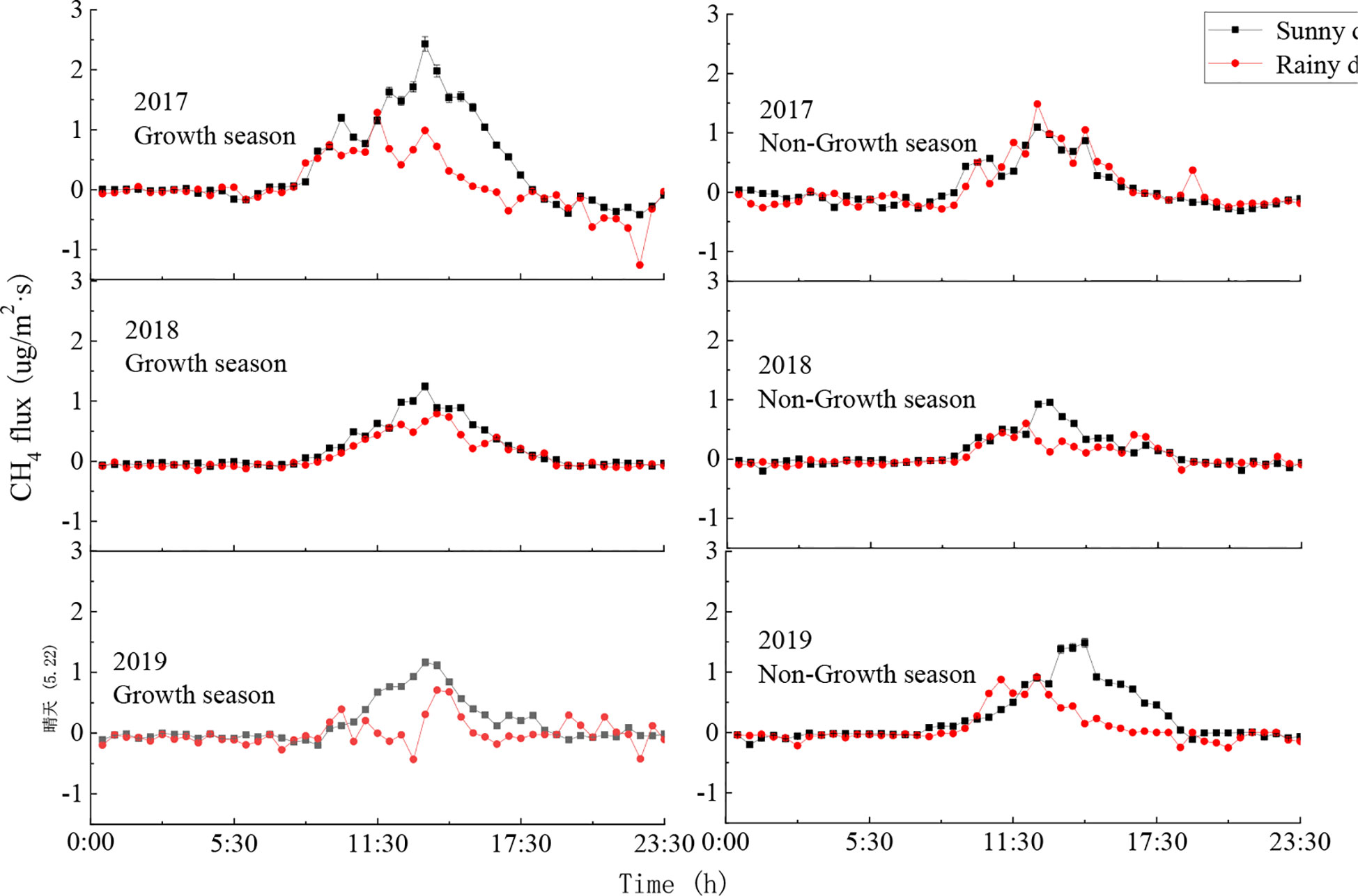
Figure 6 Diurnal variations of CH₄ flux on sunny and rainy days. Error bars show standard deviation.

During the growth season, CH₄ flux was positive during the day and showed no significant changes during the night. The daily average CH₄ fluxes on a typical sunny day in 2017, 2018, and 2019 were respectively 0.38 μg·m^-2·s^-1, 0.12 μg·m^-2·s^-1, and 0.16 μg·m^-2·s^-1, while the daily average CH₄ fluxes on a typical rainy day were respectively 0.06 μg·m^-2·s^-1, 0.05 μg·m^-2·s^-1, and 0.27 μg·m^-2·s^-1. During the non-growth season, the daily average CH₄ fluxes on a typical sunny day in 2017, 2018, and 2019 were respectively 0.07 μg·m^-2·s^-1, 0.19 μg·m^-2·s^-1, and 0.25 μg·m^-2·s^-1, while the daily average CH₄ fluxes on a typical rainy day were respectively 0.08 μg·m^-2·s^-1, 0.10 μg·m^-2·s^-1, and 0.08 μg·m^-2·s^-1. The CH₄ fluxes were higher on sunny days than on rainy days and reached maximum values in the afternoons on sunny days. In contrast, the CH₄ flux on a rainy day reached its maximum value before noon.

Typical sunny days showed generally consistent changes in CH₄ flux throughout the day, while the flux changes on rainy days differed depending on precipitation intensity and amount. During the growth season, the CH₄ flux on sunny days was slightly higher than on rainy days due to the larger leaf area caused by rainfall. During the non-growth season, both duration and amount of rainfall were reduced, such that CH₄ flux did not differ significantly between rainy and sunny days. Overall, CH₄ flux during the day was positive, making the ecosystem a CH₄ source, and CH₄ flux at night was negative, making the ecosystem a CH₄ sink.

3.2.1.3 Diurnal variations of CH₄ flux during continuous rain

CH₄ fluxes before, during, and after periods of continuous rain in 2017, 2018, and 2019 were summarised. The precipitations in these periods were respectively 127.2 mm, 77.7 mm, and 220.5 mm. Figure 7 shows the diurnal cycle of CH₄ flux for each continuous rainfall period.

FIGURE 7

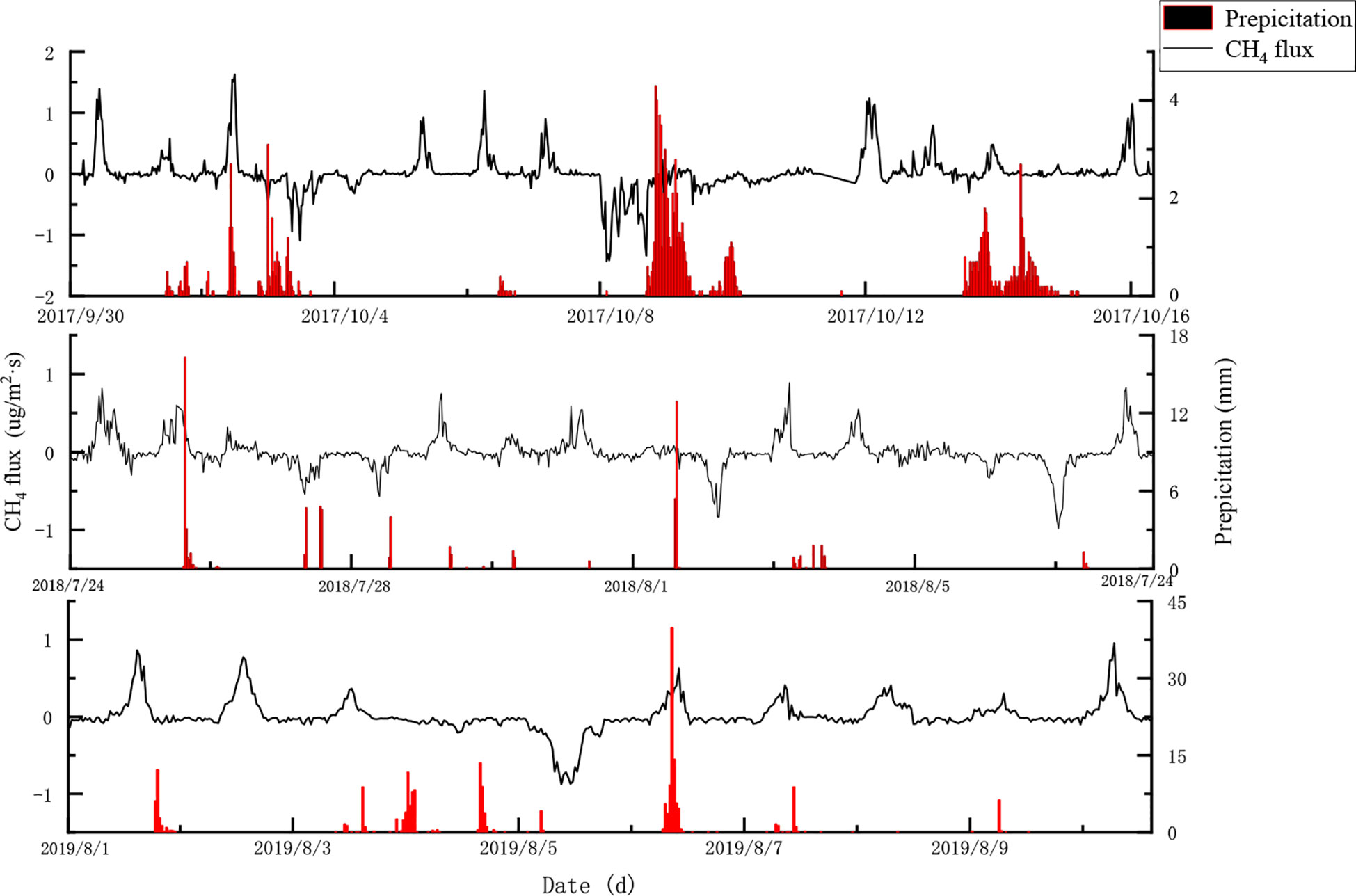
Figure 7 Within-day changes in CH₄ flux of ecosystem during periods of continuous rainfall.

Considering the period before the rain began (to Sep 30^th) and after rainfall (Oct 16^th) were sunny days, the diurnal variation in CH₄ flux was consistent with the forest being a CH₄ source in the daytime and a CH₄ sink at night. At the beginning of the continuous rainfall period (Oct 1^st to 2^nd), CH₄ flux had no change with a precipitation of 12.8 mm; however, the CH₄ flux exhibited a U-shaped pattern and became a CH₄ sink during Oct 3^rd and 4^th (precipitation 13.6 mm). The CH₄ flux on October 5^th to 7^th (precipitation 1.6 mm) again changed consistently to become a CH₄ source. The CH₄ flux again exhibited a U-shaped pattern on October 8^th (precipitation 0.1 mm) and served as a CH₄ sink, but showed no significant changes from October 9^th to 11^th (precipitation 62.7 mm). With precipitation 0.1 mm on October 12^th, CH₄ flux showed the same pattern as on a sunny day, while during October 13^th to 15^th it changed a little (precipitation 36.3 mm). The diurnal dynamic of CH₄ flux showed similarities with June 24^th to August 9^th in 2018 and August 1^st to 10^th in 2019 and exhibited an alternation of source/sink.

The continuous rainfall had a significant impact on the within-day changes of CH₄ flux, through influences on atmospheric temperature, air humidity, soil temperature, and soil humidity. There was a lag of approximately 3 to 4 days between the rainfall and its influence on CH₄ flux which ultimately led to the source-sink transition of the ecosystem. This means that if the rainfall continued for 3 to 4 days, the ecosystem transformed from a CH₄ source to a CH₄ sink. The intensity and duration of the rainfall had a coupled effect on the CH₄ flux, which further influenced the CH₄ source-sink transition of the ecosystem.

3.2.2 Seasonal changes in the CH₄ flux of the ecosystem

The CH₄ flux of the ecosystem showed obvious seasonal changes (Figure 8). It increased from November to March the following year, and gradually decreased thereafter, reaching a minimum in June, and again increased during July and August, and decreased in September until it reached the year-round minimum in October. These changes are mainly due to the radiation, temperature, precipitation, and vegetation growth during the different months. For example, between January and March in 2017, which is the non-growth season, soil and vegetation branches released CH₄, causing the forest ecosystem to serve as a CH₄ source from which the maximum emission of CH₄ was reached in March (4.47 g·m^-2·month^-1). Between April and June in 2017, due to the increase in solar radiation, temperature, and hence leaf area, the CH₄ flux of the ecosystem gradually reduced, until it reached the first minimum value in June (2.55 g·m^-2·month^-1, 1.857 g·m^-2·month^-1). July was the start of the rainy season, a period during which the soil moisture increased, causing CH₄ flux to increase accordingly. It reached a maximum in August (3.5 g·m^-2·month^-1). Subsequently, CH₄ flux decreased as the intensity and frequency of precipitation reduced, until the year-round minimum was reached in October (0.33 g·m^-2·month^-1).

FIGURE 8

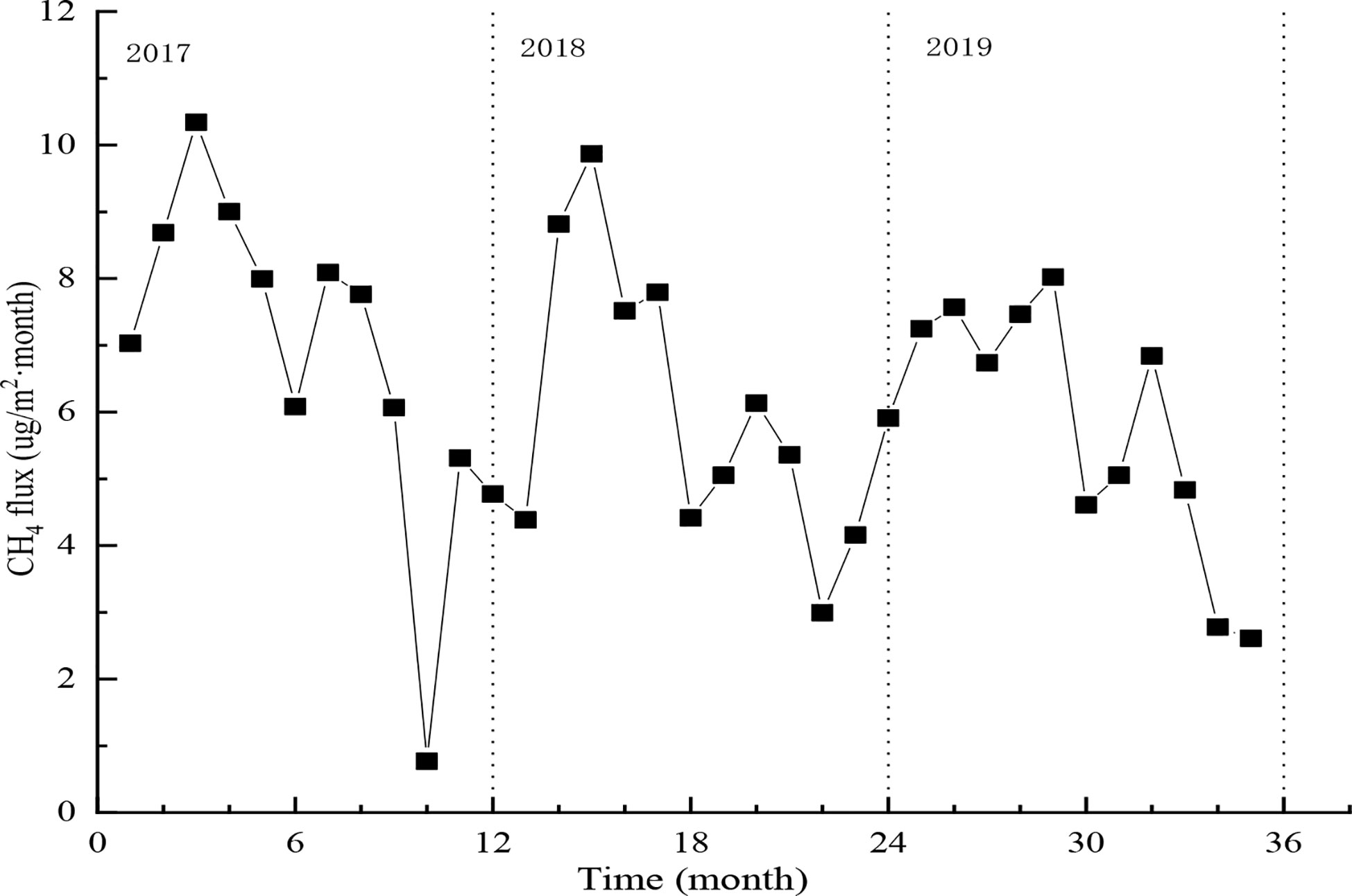
Figure 8 Seasonal changes in CH₄ flux of ecosystem.

The ranges of CH₄ emissions were 0.008–0.108 g C·m^-2·month^-1, 0.031–0.103 g C·m^-2·month^-1, and 0.027–0.084 g C·m^-2·month^-1 respectively in 2017, 2018, and 2019, with the year-round change in CH₄ emissions being respectively 3.31 g C·m^-2·year ^-1, 2.81 g C·m^-2·year ^-1, and 2.94 g C·m^-2·year^-1, corresponding to an annual average of 3.02 g C·m^-2·year^-1. Total annual emissions of CH₄ were lowest in 2018, mainly due to the higher precipitation of that year (647.8 mm) in comparison to 2017 and 2019.

4 Discussion

According to micro-meteorological theory, CH₄ flux data taken from locations with a wide underlying surface of flat terrain and uniform canopy can reflect the actual average CH₄ flux of the ecosystem. However, most observation locations do not have the ideal underlying surface, making it necessary to analyse the spatial representation of the flux observation of the complex underlying surface in the flux data. Therefore, quantitative evaluation of the flux footprint is the basis for a correct understanding of the data; this can be achieved by using the eddy covariance method. An in-depth understanding of the spatial representation of the flux towers and an accurate evaluation of the spatiotemporal distribution of flux footprints can help to obtain a more thorough understanding of the CH₄ flux sources in the ecosystem.

The flux footprint was heavily influenced by environmental factors such as atmospheric stability, wind speed and direction, atmospheric temperature, underlying surface roughness, and zero plane displacement (Leclerc and Thurtell, 1990; Kljun et al., 2002). In particular, atmospheric stability directly affects the distribution of flux footprint. In this chapter, the results of analysis of wind direction and speed data from 2017 to 2019 were described. These revealed that the study area mainly experienced east and west-south-westerly winds. Regardless of growth or non-growth season, the footprint was smaller when the atmosphere was unstable. This can be explained by the turbulent airflow between the underlying surface and the atmosphere. and the fast exchange of material in the vertical direction, which cause the flux measurements from the windward sites to be greatly affected by the underlying surface. However, the leaf area index is lower during the non-growth season, causing the flux measurements to be taken from sites further downwind, and as a result, the footprint during the non-growth season was larger than that during the growth season. This result is consistent with the results from other ecosystems such as farmland, desert, and grassland (Zhou et al., 2014; Feng et al., 2017; Zhou et al., 2018).

A variety of evidence now makes it clear that all biological surfaces in upland forests have the potential to exchange CH₄. This included reports of novel sources of CH4 emissions in nominally upland ecosystems, eddy flux evidence of hot spots or hot moments of forest CH₄ emissions. Clear CH₄ diurnal variation of the ecosystem exchange showed an inverted U-shape pattern. The CH₄ flux of the ecosystem after sunrise were a CH₄ source for the atmosphere due to the increase in radiation and temperature, and reached its maximum around 15:00. While after sunset, the CH₄ flux showed a CH₄ sink and had a little change due to the weak turbulence at night. This trend is consistent with the results published by Nakai et al. (2020), but the opposite of what Ueyama et al, 2013 had discovered. Covey and Megonigal (2018) and Pitz and Megonigal (2017) found that tree branches, live or dead alike, were potential CH₄ sources in montane forests. Machacova et al. (2016) suggested that the branches and stems of mature Pinus sylvestris in southern Finland emit CH₄. The current study found that CH₄ emissions increased sharply before noon and decreased gradually in the afternoon during spring and summer as the temperature in the afternoon was higher, which is consistent with the results published by Korkiakoski et al., 2017. Without atmospheric stability, CH₄ flux is related to temperature to a certain extent. In addition, CH₄ flux during daytime is also dependent on factors such as soil moisture. Precipitation is greater during the growth season, causing the daily average CH₄ fluxes during the growth season to be greater than those during the non-growth season. The daily average CH₄ flux was greatest in March and lowest in October. The CH₄ flux changed from sink to source around 8:30 each day in July, which was the earliest among all months, and around 10:00 in November, which was the latest among all months. The CH₄ flux changed from source to sink around 19:30 during July and August, which was the latest among all months. This change became earlier starting from September, until the transition took place around 18:00 in December. Consequently, the duration that the CH₄ flux remained positive was longest in July (11 h) and shortest in October (8 h). This finding is similar to the results published by Querino et al. (2011), who discovered that the duration of positive CH₄ flux was longer than in a tropical forest ecosystem after sunrise (5 h). Gao et al. (2016) found that positive CH₄ flux was measured during the daytime during some months in a floodplain plantation ecosystem, which may have been due to the CH₄ gas stored in the canopy during night-time being released into the atmosphere after sunrise.

The diurnal variations of CH₄ fluxes in this ecosystem showed obvious trends during the growth and non-growth seasons, being positive during daytime and with non-significant changes at night. This indicates that the CH₄ flux showed significant changes only when the atmosphere was unstable and the turbulent airflow was strong; at night, when the atmosphere was stable and the turbulent airflow was weak, the CH₄ flux showed no significant changes. This is consistent with research on night-time CH₄ flux in farmland and wetland ecosystems (Song et al., 2019; Zhang et al., 2019). The maximum values of diurnal average CH₄ fluxes during the growth season were all less than those of the non-growth season, mainly because of the larger precipitation and net radiation, the latter of which enhanced plants’ activities and reduced the oxidation of CH₄ (Praeg et al., 2019). Obvious daily changes were observed during the sunny days in both the growth and the non-growth season. The CH₄ fluxes were greater on a sunny day than on a rainy day, and the maximum value appeared in the afternoon; in contrast, CH₄ flux changed in complicated ways on rainy days, when the maximum value appeared before noon, and the daily average was slightly lower. Although soil appears to be a CH₄ sink during the growth season (Zhuang et al, 2016), the emissions from plants may have offset the effect of the soil CH₄ sink (Pitz and Megonigal, 2017; LeMer and Roger, 2001).

The comparison of diurnal variations of CH₄ flux before, during, and after continuous rainfall indicated that the intensity and frequency of rainfall, as well as extreme precipitation events, influenced the CH₄ source-sink transition. Before and after the rainfall, the CH₄ flux changed in the same manner as on a typical sunny day. Due to the lag in the influence of rainfall on the CH₄ flux, the daily patterns of CH₄ flux only began to change on the third or fourth day of continuous rainfall. They then followed a U-shaped pattern with a negative value during daytime, causing the ecosystem to serve as a CH₄ sink. As the rainfall continued for more days, the CH₄ source-sink transition happened approximately every three days. This can be explained by the change in effective dynamic characteristics of soil moisture according to water intake; this being most affected by limited water intake, while the more frequently precipitation events occur, the more dependent soil moisture is on water intake (Zhao et al., 2015).

The CH₄ flux of this ecosystem showed obvious seasonal changes. As radiation and temperature increased, plants entered the growth season and the leaf area of the canopy increased, causing the CH₄ flux to gradually increase, reaching a year-round maximum in March. As the leaf area continued to increase with radiation, the CH₄ flux gradually decreased, until it reached the first minimum in June when the temperature is high and precipitation is low and the physiological activities of the plants can be affected. The rain season started in July or August, causing the soil moisture and hence the CH₄ flux to increase. Both radiation and temperature decreased after August, and the CH₄ flux decreased correspondingly. In October, due to the continuous rainfall, the CH₄ flux reached a year-round minimum. The magnitude of the CH₄ flux among the seasons was observed in the order of spring > summer > winter > autumn, which is consistent with the results reported by Zona et al. (2013). Zhang et al. (2019) studied the poplar plantations in the Hongze Lake area and found that weak CH₄ absorption was observed during the growth season, while weak CH₄ emissions were observed during the non-growth season, causing the ecosystem to serve as a weak CH₄ sink in a year overall. However, the CH₄ flux of the ecosystem studied between 2017 and 2019 and reported in this paper had an average of 3.02 g C·m^-2·year^-1, indicating that the ecosystem was a weak CH₄ source, which is inconsistent with the results by Zhang et al. (2019). This inconsistency may be due to the length of study period, climate, and types of trees.

The study revealed that the mixed plantation forest ecosystem in warm temperate continental is methane source, which is consistent with the results of the boreal forests in the United State (Nakai et al., 2020). During the period of 2016 to 2019, the average daily and annual CH₄ flux was 0.019g C·m^-2·day^-1 lower than that of tropical Alan Batu forest, temperate boreal forest ecosystem, subtropical Pinus ponderosa forest and temperate black spruce forest ecosystem (Wong et al., 2018; Nakai et al., 2020; Iwata et al., 2015; Smeets et al., 2009), similar to subtropical plantation ecosystem in China (Gao et al., 2016). It was higher than temperate boreal forest (Ueyama et al., 2013), with the mainly because of the observation methods (Table 1). Climate, soil and tree species in different regions are important reasons for CH₄ fluxes, as well as differences in measurement methods and CH₄ source intensity or magnitude.

TABLE 1

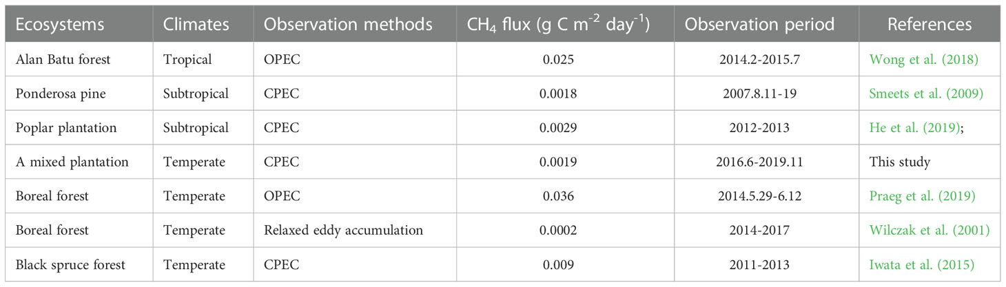
Table 1 Mean daily CH₄ flux measured using the eddy covariance method from different ecosystems in Ameirco, Europe, and Asia.

5 Conclusion

The flux footprint showed non-uniform changes throughout a day and were smaller in the growth season and daytime, reaching a minimum at noon and a maximum at 3 am. The eddy covariance measurement system measures the size of the windward flux footprint, and the data represented the flux of the study area well.

The CH₄ flux showed obvious patterns in its daily changes. The within-day changes in CH₄ flux by month followed an inverted U-shape pattern which was source during daytime and a CH₄ sink at night. The largest daily average CH₄ flux appeared in March, and the smallest appeared in October.

The CH₄ flux also showed obvious seasonal changes. The CH₄ flux reached its maximum in spring, and the first minimum of the year was observed in summer, followed by the year-round minimum in autumn. The flux gradually increased in winter but was still lower than in summer.

Precipitation events affected the CH₄ source-sink transition with a time lag. The changes in within-day CH₄ flux began on the third and fourth day of continuous rainfall, and were negative during the daytime (i.e., it was a CH₄ sink). As rainfall continued, the CH₄ source-sink transition alternated approximately every three days.

The CH₄ source-sink status of the ecosystem was relatively complicated. Overall, the ecosystem was a weak CH₄ source, while the source-sink transition occurred on a daily basis.

Based on the observation data of three years, this paper reports on analyses of the characteristics of changes in the CH₄ fluxes in the ecosystem. To reduce the uncertainty in evaluating the CH₄ flux of the ecosystem, continuous observation and measurement are required.

Data availability statement

The raw data supporting the conclusions of this article will be made available by the authors, without undue reservation.

Author contributions

WY and HH carried out the data processing and analysis and wrote the manuscript; JZ, PM, JL, and TW contributed to the conception and design of the study; FZ and QP organised the data and performed the statistical analysis. All authors participated in the manuscript editing and approved the final version.

Funding

This research was financially supported by the Special Project on National Science and Technology Basic Resources Investigation of China (2021FY100701).

Acknowledgments

We thank Dr. Ning Zheng and Mr. Quan Yang for their assistance with field measurements and instrumentation maintenance.

Conflict of interest

The authors declare that the research was conducted in the absence of any commercial or financial relationships that could be construed as a potential conflict of interest.

Publisher’s note

All claims expressed in this article are solely those of the authors and do not necessarily represent those of their affiliated organizations, or those of the publisher, the editors and the reviewers. Any product that may be evaluated in this article, or claim that may be made by its manufacturer, is not guaranteed or endorsed by the publisher.

References

Baer, D. S., Paul, J. B., Gupta, J. B., O'Keefe, A. (2002). Sensitive absorption measurements in the near-infrared region using off-axis integrated-cavity-output spectroscopy. Appl. Phys. B-Lasers Optics 75 (2-3), 261–265. doi: 10.1007/s00340-002-0971-z

CrossRef Full Text | Google Scholar

Covey, K. R., Megonigal, J. P. (2018). Methane production and emissions in trees and forests. New Phytol. 222, 35–51. doi: 10.1111/nph.15624

CrossRef Full Text | Google Scholar

Falge, E., Baldocchi, D., Olson, R., Anthoni, P., Aubinet, M., Bernhofer, C., et al (2001). Gap filling strategies for defensible annual sums of net ecosystem exchange. Agric. For. Meteorol. 107, 43–69. doi: 10.1016/S0168-1923(00)00225-2

CrossRef Full Text | Google Scholar

Feng, J. T., Hu, Z. H., Zhang, B. Z., Zhou, Q. Y., Peng, Z. G. (2017). Analyzing flux footprint of agro-ecosystem measured by the eddy covariance system. J. Irrigation Drainage 036, 49–56. doi: 10.13522/j.cnki.ggps.2017.06.010

CrossRef Full Text | Google Scholar

Frankenberg, C., Meirink, J. F., van Weele, M., Platt, U., Wagner, T. (2005). Assessing methane emissions from global space-bome observations. Science 308, 1010–1014. doi: 10.1126/science.1106644

PubMed Abstract | CrossRef Full Text | Google Scholar

Gao, S. H., Zhang, X. D., Tang, Y. X., Chen, J. Q., Tang, J., Sun, Q. X. (2016). Dynamics and regulation of CH4 flux in a poplar plantation on a floodplain. Acta Ecologica Sin. 36 (18), 5912–5921. doi: 10.5846/stxb201503220546

CrossRef Full Text | Google Scholar

He, F. J., Han, H. B., Ma, X. Q., Zhang, J. S., Sun, S. J. (2019). Characteristics and influence factors of CH4 flux in different areas of longbaotan marsh wetland. Ecol. Environ. Sci. 28 (4), 803–811. doi: 10.16258/j.cnki.1674-5906.2019.04.020

CrossRef Full Text | Google Scholar

Ibrom, A., Dellwik, E., Flyvbjerg, H., Jensen, N. O., Pilegaard, K. (2007a). Strong low-pass filtering effects on water vapour flux measurements with closed-path eddy correlation systems. Agric. For Meteorol 147, 140–156. doi: 10.1016/j.agrformet.2007.07.007

CrossRef Full Text | Google Scholar

Ibrom, A., Dellwik, E., Larsen, S. E., Pilegaard, K. (2007b). On the use of the Webb-Pearman-Leuning theory for closed-path eddy correlation measurements. Tellus 59B, 937–946. doi: 10.1111/j.1600-0889.2007.00311.x

CrossRef Full Text | Google Scholar

IPCC (2013). Climate change 2013: The physical science baswas. contribution of working group I to the fifth assessment report of the intergovernmental panel on climate change. Comput. Geometry [J] 18, 95–123.

Google Scholar

Iwata, H., Harazono, , Ueyama, Y. M., Sakabe, A., Nagano, H., Kosugi, Y., et al (2015). Methane exchange in a poorly-drained black spruce forest over permafrost observed using the eddy covariance technique. Agric. For. Meteorol. 214, 157–168. doi: 10.1016/j.agrformet.2015.08.252

CrossRef Full Text | Google Scholar

Kljun, N., Rotach, M. W., Schmid, H. P. (2002). A three-dimensional backward Lagrangian footprint model for a wide range of boundary-layer stratifications. Boundary-Layer Meteorology 103 (2), 205–226. doi: 10.1023/a:1014556300021

CrossRef Full Text | Google Scholar

Korkiakoski, M., Tuovinen, J. P., Aurela, M., Koskinen, M., Minkkinen, K., Ojanen, P., et al (2017). Methane exchange at the peatland forest floor -automatic chamber system exposes the dynamics of small fluxes. Biogeosciences 14, 1947–1967. doi: 10.5194/bg-14-1947-2017

CrossRef Full Text | Google Scholar

Leclerc, M. Y., Thurtell, G. W. (1990). Footprint prediction of scalar fluxes using a markovian analysis. Boundary-Layer Meteorology 52 (3), 247–258. doi: 10.1007/bf00122089

CrossRef Full Text | Google Scholar

LeMer, J., Roger, P. (2001). Production, oxidation, emission and consumption of methane by soils: a review. Eur. J. Soil Biol. 37, 25–50. doi: 10.1016/S1164-5563(01)01067-6

CrossRef Full Text | Google Scholar

Machacova, K., Back, J., Vanhatalo, A., Halmeenmäki, F., Kolari, P., Mammarella, I., et al (2016). Pinus sylvestras as a missing source of nitrous oxide and methane in boreal forest. Sci. Rep. 6, 23410. doi: 10.1038/srep23410

PubMed Abstract | CrossRef Full Text | Google Scholar

Mauder, M., Foken, T. (2004). Documentation and instruction manual of the eddy covariance software package tk2 (Tech. rep.) (Uni-versitt Bayreuth: Abt. Mikrometeorologie).

Google Scholar

Megonigal, J. P., Guenther, A. (2008). Methane emissions from upland forest soils and vegetation. Tree Physiol. 28, 491–498. doi: 10.1093/treephys/28.4.491

PubMed Abstract | CrossRef Full Text | Google Scholar

Mikkelsen, T. N., Bruhn, D., Ambus, P., Larsen, K. S., Ibrom, I., Pilegaard, K. (2012). Is methane released from the forest canopy? iForest - Biogeosciences Forestry 4 (5), 200–204. doi: 10.3832/ifor0591-004

CrossRef Full Text | Google Scholar

Miyama, T., Hadhimoto, T., Kominami, Y., Nakagawa, K., Okumura, M., Tohno, S. (2010). Temporal and spatial variations in CH4 concentrations in a Japanese warm-temperate mixed forest. J. Agric. Meteorology 66 (1), 1–9. doi: 10.2480/agrmet.66.1.1

CrossRef Full Text | Google Scholar

Nakai, T., Hiyama, T., Petrov, R. E., Kotani, A., Ohtaf, T., Maximovde, T. C. (2020). Application of an open-path eddy covariance methane flux measurement system to a larch forest in eastern Siberia. Agric. For. Meteorology 282-283, 107860. doi: 10.1016/j.agrformet.2019.107860

CrossRef Full Text | Google Scholar

Pitz, S., Megonigal, J. P. (2017). Temperate forest methane sink diminished by tree emissions. New Phytol. 214 (4), 1432–1439. doi: 10.1111/nph.14559

PubMed Abstract | CrossRef Full Text | Google Scholar

Praeg, N., Schwinghammer, L., Illmer, P. (2019). Larix decidua and additional light affect the methane balance of forest soil and the abundance of methanogenic and methanotrophic microorganisms. FEMS Microbiol. Lett. 366 (24), 1–10. doi: 10.1093/femsle/fnz259

CrossRef Full Text | Google Scholar

Querino, C., Smeets, C., Vigano, I., Holzinger, R., Moura, V., Gatti, L. V., et al (2011). Methane flux, vertical gradient and mixing ratio measurements in a tropical forest. Atmospheric Chem. Phys. 11 (15), 7943–7953. doi: 10.5194/acp-11-7943-2011

CrossRef Full Text | Google Scholar

Shoemaker, J. K., Keenan, T. F., Hollinger, D. Y., Richardson, A. D. (2014). Forest ecosystem changes from annual methane source to sink depending on late summer water balance. Geophys. Res. Lett. 41, 673–679. doi: 10.1002/2013GL058691

CrossRef Full Text | Google Scholar

Simpson, I. J., Edwards, G. C., Thurtell, G. W. (1999). Variations in methane and nitrous oxide mixing ratios at the southern boundary of a Canadian boreal forest. Atmospheric Environ. 33, 1141–1150. doi: 10.1016/s1352-2310(98)00235-0

CrossRef Full Text | Google Scholar

Smeets, C. J. P. P., Holzinger, R., Vigano, I., Goldstein, A. H., Röckmann, T. (2009). Eddy covariance methane measurements at a ponderosa pine plantation in California. Atmospheric Chem. Phys. 9 (21), 8365–8375. doi: 10.5194/acp-9-8365-2009

CrossRef Full Text | Google Scholar

Song, C. Q., Liu, W., Lu, H. B., Yuan, W. P. (2019). Characteristics and drivers of methane fluxes from a rice paddy based on the flux measurement. Adv. Earth Sci. 34 (11), 1141–1151. doi: 10.11867/j.issn.1001-8166.2019.11.1141

CrossRef Full Text | Google Scholar

Sundqvist, E., Mölder, M., Crill, P., Kljun, N., Lindroth, A. (2015). Methane exchange in arboreal forest estimated by gradient method. Tellus B 67, 26688. doi: 10.3402/tellusb.v67.26688

CrossRef Full Text | Google Scholar

Tong, X. J., Meng, P., Zhang, J. S., Li, J., Zheng, N., Huang, H. (2012). Ecosystem carbon exchange over a warm-temperate mixed plantation in the lithoid hilly area of the north China. Atmospheric Environ. 49, 257–267. doi: 10.1016/j.atmosenv.2011.11.049

CrossRef Full Text | Google Scholar

Ueyama, M., Takai, Y., Takahashi, Y., Ide, R., Hamotani, K., Kosugi, Y., et al (2013). High-precision measurements of the methane flux over a larch forest based on a hyperbolic relaxed eddy accumulation method using a laser spectrometer. Agric. For. Meteorology 178-179, 183–193. doi: 10.1016/j.agrformet.2013.04.029

CrossRef Full Text | Google Scholar

Ueyama, M., Yoshikawa, K., Takagi, K. (2018). A cool-temperate young larch plantation as a net methane source - a 4-year continuous hyperbolic relaxed eddy accumulation and chamber measurements. Atmos. Environ. 184, 110–120. doi: l0.1016/j.atmosenv.2018.04.025

Google Scholar

Vickers, D., Mahrt, L. (1997). Quality control and flux sampling problems for tower and aircraft data. J. Atmos Oceanic Technol. 14, 512–526. doi: 10.1175/1520-0426(1997)014<0512:QCAFSP>2.0.CO;2

CrossRef Full Text | Google Scholar

Wilczak, J. M., Onclcy, S. P., Stage, S. A. (2001). Sonic anemometer tilt correction algorithms. Bound. Lay. Meteorol 106, 85–106. doi: 10.1023/A:1018966204465

CrossRef Full Text | Google Scholar

Wong, G. X., Hirata, R., Hirano, T., Kiew, F., Aeries, E. B., Musin, K. K., et al (2018). Micrometeorological measurement of methane flux above a tropical peatswamp fores. Agric. For. Meteorol. 256, 353–361. doi: 10.1016/j.agrformet.2018.03.025

CrossRef Full Text | Google Scholar

Yuan, W., Zhang, J., Meng, P., Tong, X. J., Pan, Q. M., He, F. J., et al (2019). Comparison of CH4 flux measurement by open- and close- path eddy covariance system. Chin. J. Agrometeorology 40 (11), 669–677. doi: CNKI:SUN:ZGNY.0.2019-11-001

Google Scholar

Zhang, Y., Feng, H. L., Wang, W. F., Xue, J. H., Wu, Y. B., Yu, Y. Q. (2019). Diurnal and seasonal changes of fluxes over a poplar plantation in hongze lake basin. J. Nanjing Forestry Univ. (Natural Sci. Edition) 43 (5), 113–120. doi: 10.3969/j.issn.1000-2006.201806032

CrossRef Full Text | Google Scholar

Zhao, R., Li, X. J., Zhao, Y., Yang, T. H., Li, G. (2015). CO2 efflux from two types of biologically crusted soil in response to simulated precipitation pules in the tengger desert. J. Desert Res. 35 (2), 393–399. doi: 10.1016/s1002-0160(17)60307-2

CrossRef Full Text | Google Scholar

Zheng, N., Zhang, J. S., Meng, P., Huang, H., Gao, J., Jia, C. R., et al (2010). Distribution of flux source area and footprint for the scintillation method over a mixed plantation in the hilly zone of the north China. Adv. Earth Sci. 25 (11), 1175–1186. doi: 10.11867/j.issn.1001-8166.2010.11.1175

CrossRef Full Text | Google Scholar

Zhou, Q., Wang, P. H., Wang, Q., Zheng, C. L., Xu, L. (2014). A footprint analysis on a desert ecosystem in West China. J. Desert Res. 34 (1), 98–107. doi: 10.7522/j.issn.1000-694X.2013.00289

CrossRef Full Text | Google Scholar

Zhou, M., Zheng, W., Gao, Q. Z. (2018). Flux footprint analysis of suburban lawn in zhuhai city. Acta Scientiarum Naturalium Universitatis Sunyatseni 57 (03), 24–33. doi: 10.13471/j.cnki.acta.snus.2018.03.004

CrossRef Full Text | Google Scholar

Zhuang, J. J., Zhang, J. S., Meng, P., Zheng, N., Li, J. X. (2016). Change of soil CH4 fluxes of robinia pseudoacacia stand during non-growing season and the impact factors. For. Res. 29 (2), 274–282. doi: CNKI:SUN:LYKX.0.2016-02-021

Google Scholar

Zona, D., Janssens, I. A., Aubinet, M., Gioli, B., Vicca, S., Fichot, R., et al (2013). Fluxes of the greenhouse gases (CO2, CH4 and N2O) above a short-rotation poplar plantation after conversion from agricultural land. Agric. For. Meteorology 169, 100–110. doi: 10.1016/j.agrformet.2012.10.008

CrossRef Full Text | Google Scholar