Forecasting Root-Zone Electrical Conductivity of Nutrient Solutions in Closed-Loop Soilless Cultures via a Recurrent Neural Network Using Environmental and Cultivation Information

In existing closed-loop soilless cultures, nutrient solutions are controlled by the electrical conductivity (EC) of the solution. However, the EC of nutrient solutions is affected by both growth environments and crop growth, so it is hard to predict the EC of nutrient solution. The objective of this study was to predict the EC of root-zone nutrient solutions in closed-loop soilless cultures using recurrent neural network (RNN). In a test greenhouse with sweet peppers (Capsicum annuum L.), data were measured every 10 s from October 15 to December 31, 2014. Mean values for every hour were analyzed. Validation accuracy (R²) of a single-layer long short-term memory (LSTM) was 0.92 and root-mean-square error (RMSE) was 0.07, which were the best results among the different RNNs. The trained LSTM predicted the substrate EC accurately at all ranges. Test accuracy (R²) was 0.72 and RMSE was 0.08, which were lower than values for the validation. Deep learning algorithms were more accurate when more data were added for training. The addition of other environmental factors or plant growth data would improve model robustness. A trained LSTM can control the nutrient solutions in closed-loop soilless cultures based on predicted future EC. Therefore, the algorithm can make a planned management of nutrient solutions possible, reducing resource waste.

Introduction

Due to benefits including improved crop yield and quality, soilless cultures in greenhouses have been growing rapidly in popularity. However, most open-loop soilless cultures release drainage nutrient solutions without treatment, causing environmental pollution such as eutrophication and accumulation of heavy metals (Fargašová, 1994; Siddiqi et al., 1998; Le Bot et al., 2001; Nicoletto et al., 2017). To resolve this problem, closed-loop soilless cultures are being studied as sustainable crop cultivation systems. In commercialized closed-loop soilless cultures, nutrient solutions are controlled based on electrical conductivity (EC) because it is easily measured by sensors. Since EC of solutions shows a linear relationship with total equivalents of ions in solutions (Griffin and Jurinak, 1973), EC-based systems have been used to control nutrient solution supply.

In soilless culture systems, root-zone EC should be controlled within target range because it significantly influences the growth and quality of crops (Sonneveld and Voogt, 2009). In general, root-zone EC dynamically varies due to environmental changes and can be controlled by adjusting the concentration of nutrient solutions. In open-loop soilless culture, these EC control processes only consider the resource usage of the system (Ku and Hershey, 1991). However, in closed-loop soilless culture, the discharge of drainage is restricted. Therefore, changes in the EC and the drainage amount are directly affected by the available concentration range of supplying nutrient solutions and the amounts of water and stock solutions for replenishment (Savvas and Manos, 1999). In the EC-based closed-loop soilless culture, which conducts minimal nutrient calibration with EC, these features may affect the stability of nutrient control (Savvas and Manos, 1999; Savvas, 2002; Massa et al., 2011). In order to maintain system reliability under these limited conditions, current control processes should be determined based on the prediction of future changes, which requires an appropriate predictive model (Draeger et al., 1995). Therefore, predicting EC is important for nutrient management of closed soilless cultures.

Although various prediction methods have been developed, nutrient control systems are usually based on contemporary EC monitoring and are vulnerable to ion balance in root-zone nutrient solutions (Neto et al., 2014; Kinoshita et al., 2016). These limits result from crops influencing changes in EC and from growth environments (Dewir et al., 2005; Stutte, 2006; Shin and Son, 2016). Because root-zone nutrient solutions are affected by environmental changes within greenhouses, predicting future changes in the EC of root-zone nutrient solutions is not easy. Prediction of EC needs various environmental data and system parameters; however, EC is greatly affected by environments in a wide range of climate changes (Savvas and Manos, 1999; Savvas, 2002; Lykas et al., 2006; Massa et al., 2011; Shin et al., 2016). It is difficult to apply a control system developed in a specific region to another region of different climate conditions. In fact, no studies have attempted to predict and forecast future EC in various climate conditions.

Deep learning has been used to draw meaningful interpretations from complicated nonlinear data (Mnih et al., 2015; Silver et al., 2016). Deep learning can be used for high-level abstraction from raw data (LeCun et al., 2015). As a part of deep learning, recurrent neural networks (RNNs) are used to analyze chronological data such as for voice and video recognition and natural language processing; this method shows better accuracy than previous algorithms (Adavanne et al., 2017; Ororbia et al., 2017).

Recurrent neural network has an advantage of inputting big data of relatively long period and the length of output values is also unlimited theoretically (Hochreiter and Schmidhuber, 1997). EC in soilless culture is a chronological factor which is difficult to predict because the future EC changes are affected by the accumulation data of past environments and plant growth. To improve EC-based nutrient controls in various climate conditions, prediction of EC should be conducted based on previous environmental factors in closed-loop soilless culture systems. The objective of this study was to predict the EC of root-zone nutrient solutions in closed-loop soilless cultures using RNN algorithms.

Materials and Methods

Cultivation Conditions

A Venlo-type greenhouse at the experimental farm of Seoul National University, Suwon, Korea (37.3° N 127.0° E) was used for experiments. Three sweet pepper (Capsicum annuum L.) plants were grown in a rockwool slab and seven slabs were used per row. In this study, four cultivation lines were installed in the greenhouse, each of which is an independent closed-loop soilless culture system having mixing tank, drainage tank, and stock solutions (Figure 1). The stock solution was divided into A and B based on the PBG nutrient solution of Netherlands. One of the cultivation lines was used for the experiment. In the greenhouse, daytime temperature was maintained at 25–35°C and nighttime temperature at 17–22°C (Figure 2). Outside temperature during the experiment was at -10.8–23°C. EC of nutrient solutions was maintained at 2.6–3.0 dS⋅m^-1 and pH at 5.5–6.5. Integrated solar radiation method was applied for irrigation control. Nutrient solutions’ composition was 14.17 meq⋅L^-1 of ${\mathrm{NO}}_{\mathrm{3}}^{\mathrm{–}}$, 1.14 meq⋅L^-1 of H₂${\mathrm{PO}}_{\mathrm{4}}^{\mathrm{–}}$, 5.92 meq⋅L^-1 of K⁺, 8.85 meq⋅L^-1 of Ca²⁺, 3.17 meq⋅L^-1 of Mg²⁺, and 3.20 meq⋅L^-1 of ${\mathrm{SO}}_{\mathrm{4}}^{\mathrm{2–}}$ as macro elements; and 0.038 meq⋅L^-1 of Fe²⁺, 0.020 meq⋅L^-1 of Zn²⁺, 0.003 meq⋅L^-1 of Cu²⁺, 0.021 meq⋅L^-1 of Mn²⁺, and 0.001 meq⋅L^-1 of ${\mathrm{MoO}}_{\mathrm{4}}^{\mathrm{2–}}$ as micro elements. After irrigation event, the drainage was returned to the reservoir tank (52 cm × 26 cm × 26 cm). EC and pH in the reservoir tanks were monitored every 3 days by using a multimeter (Multi 3420 SET C, WTW, Germany). EC and water content in the root media were measured by using a TDR sensor (Grodan, WCM-control, Denmark). EC and pH of fresh water were 0.17 dS⋅m^-1 and 7.11, respectively, containing 0.21 meq⋅L^-1 of Na²⁺, 0.29 meq⋅L^-1 of Cl^-, 0.04 meq⋅L^-1 of K⁺, 0.71 meq⋅L^-1 of Ca²⁺, 0.21 meq⋅L^-1 of Mg²⁺, 0.19 meq⋅L^-1 of ${\mathrm{SO}}_{\mathrm{4}}^{\mathrm{2–}}$, 0.39 meq⋅L^-1 of ${\mathrm{NO}}_{\mathrm{3}}^{\mathrm{–}}$, and 0.04 meq⋅L^-1 of ${\mathrm{PO}}_{\mathrm{4}}^{\mathrm{3–}}$. Drainage ratios were maintained at 20–30% during experimental period. Plants were grown to maintain two main stems, which were vertically trellized to a “V” canopy system (Jovicich et al., 2004).

FIGURE 1

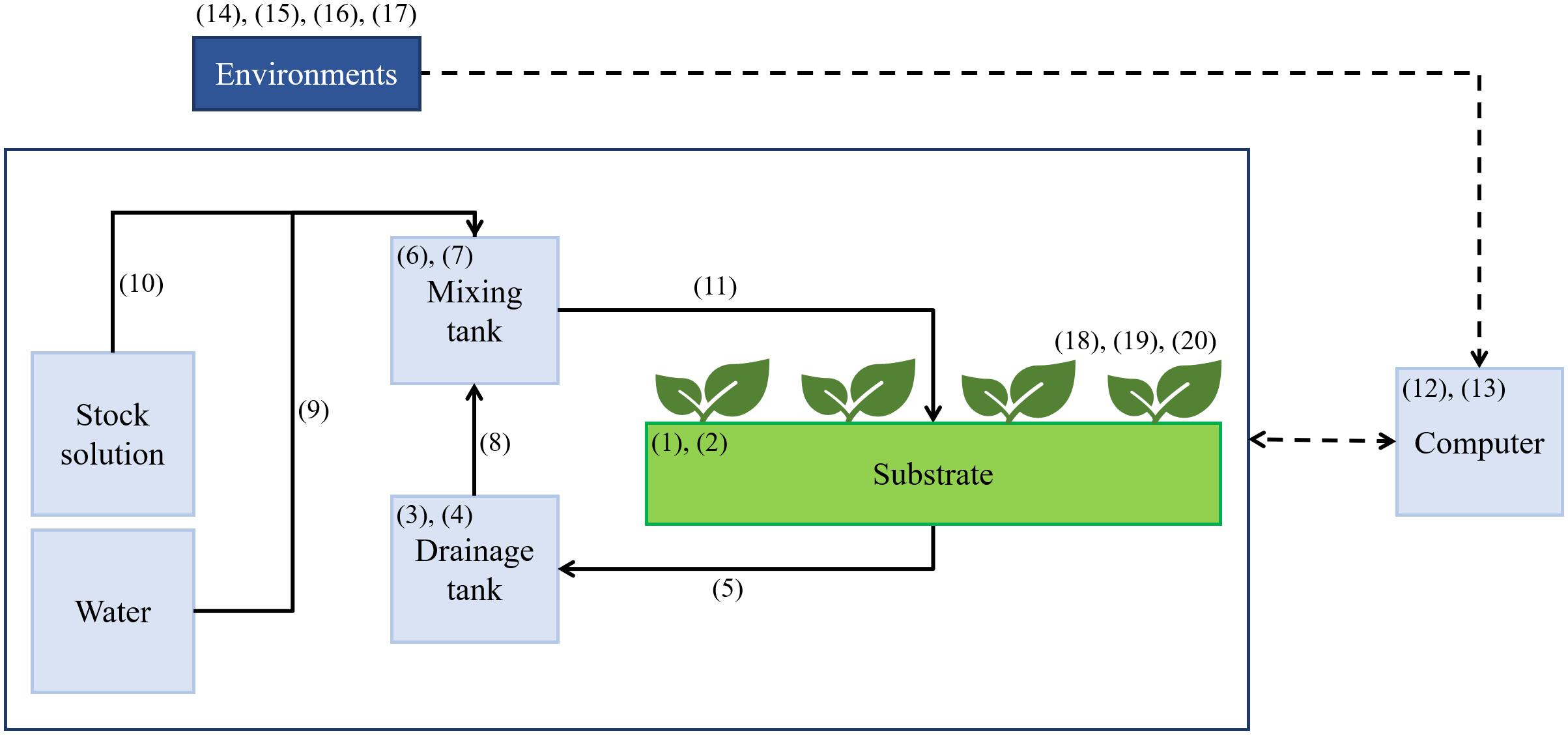
FIGURE 1. A diagram of a closed-loop soilless culture system and measured data of nutrient solutions and growth environments. Refer to Table 1 for the measured data (1–20).

FIGURE 2

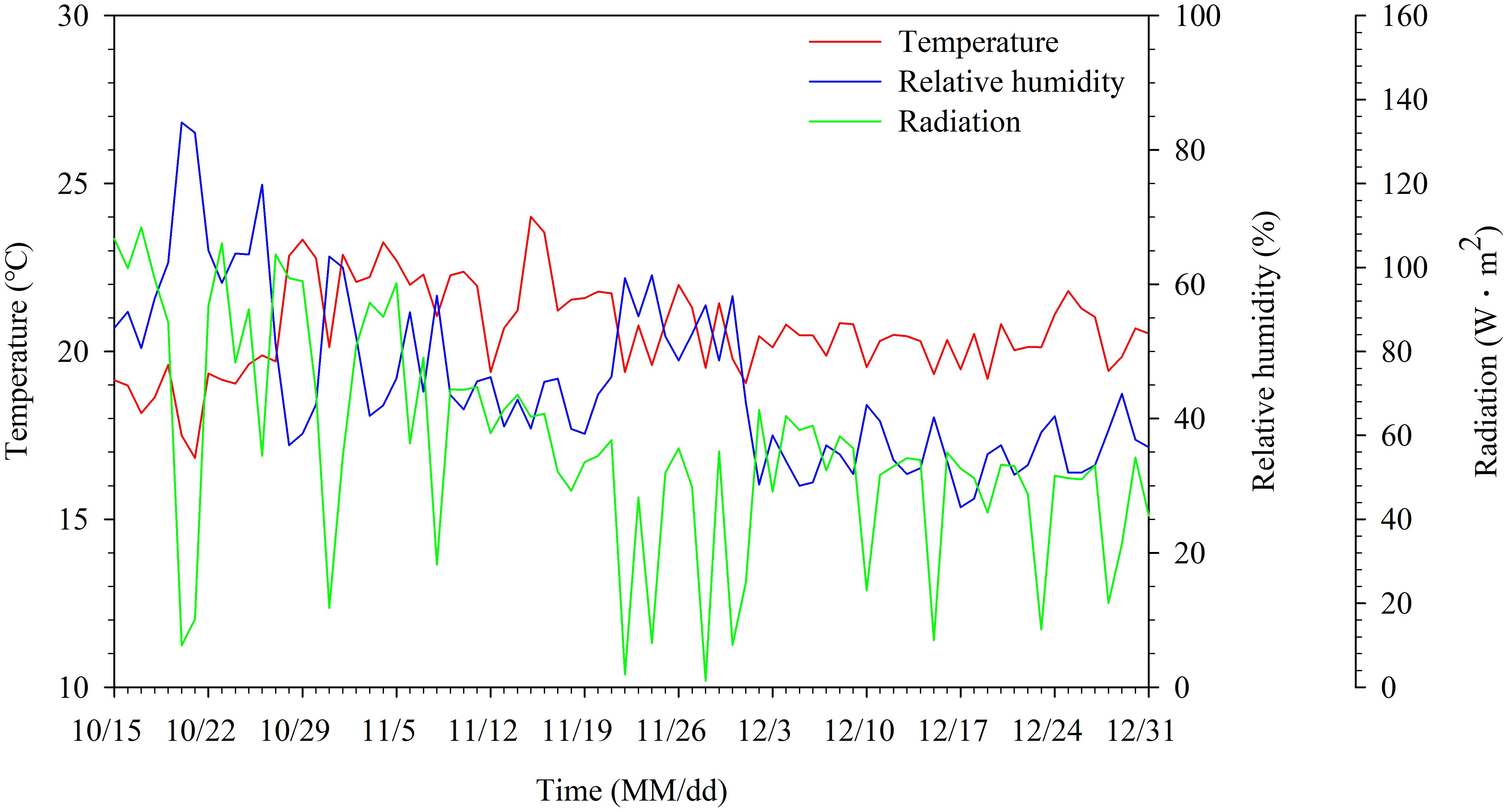
FIGURE 2. Daily averages of temperature, relative humidity, and radiation in the greenhouse from 15 October to 31 December. Zeros were excluded when radiation was averaged.

Data Collection

Data on nutrient solutions and growth environments were measured to train the algorithm (Table 1). The ECs of nutrient solutions in the mixing tank and drainage tank were measured by EC sensors (SCF-01A, DIK, Korea). The EC and moisture content of substrates were measured by a FDR sensor (CoCo 100B, Mirae Sensor, Korea). CO₂ concentration and light intensity in the greenhouse were measured by using a nondispersive infrared CO₂ sensor (KCD-AN300, Sensecube, Korea) and by a pyranometer (SP-110, Apogee, United States), respectively. Data were measured every 10 s from October 15 to December 31, 2014. Mean values for every hour were used. A total of 1,416 data points was used for this study.

TABLE 1

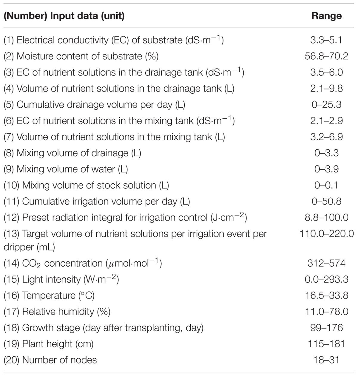
TABLE 1. Ranges of measured input data in closed-loop soilless cultures.

Recurrent Neural Network

Recurrent neural network algorithms deal with chronological data with a returning cycle. Long short-term memory (LSTM), an RNN algorithm, can solve the vanishing gradient problem of RNN (Hochreiter and Schmidhuber, 1997). This means that LSTM remembers the data of a long previous sequence. The core of LSTM algorithm is a cell with several gates (Figure 3). LSTM accepts previous data with addition operation, so vanishing gradient or exploding gradient problem is not occurred. Therefore, LSTM can analyze long time data than simple RNN.

FIGURE 3

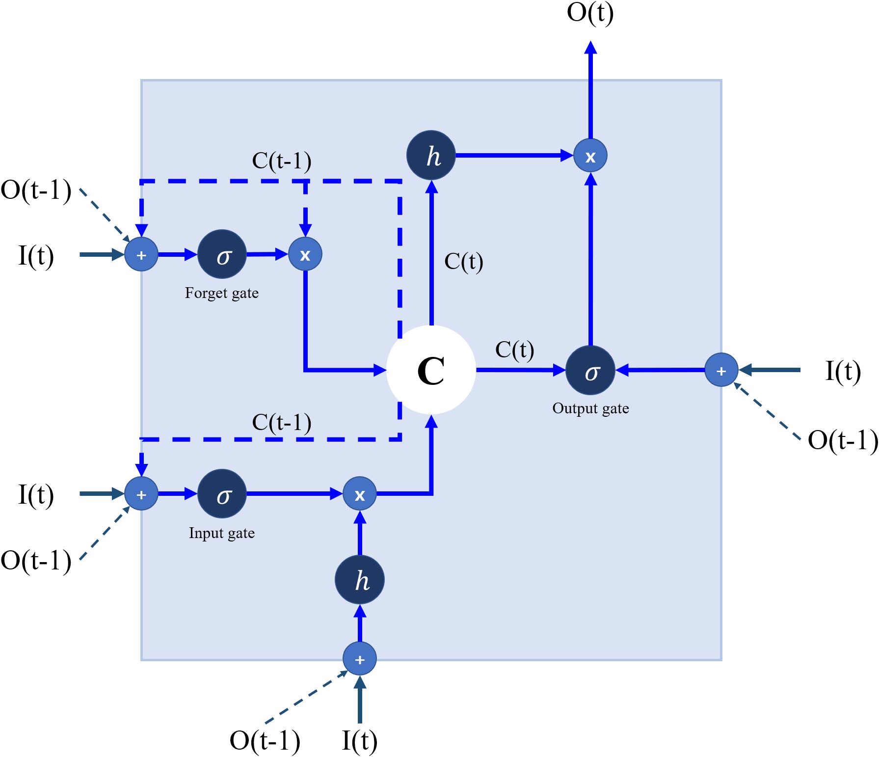
FIGURE 3. A structure of a long short-term memory (LSTM). I, input vectors; O, output vectors; C, cell state; h, tanh for input and output activation function; σ, sigmoidal function for gate activation function; t and t–1, current and previous times, respectively. Refer to Table 1 for the input (I) and output (O).

Long short-term memory cells can retain, save, and load information about previous data. LSTM receives current input and previous output simultaneously, and the received information is operated through the gates. Previous information is saved as cell state, so sequenced data can be analyzed based on cell state. Gates are divided into three parts: input, forget, and output. The input gate determines how to select the data. The forget gate decides how much data should be forgotten and passes suitably forgotten previous data through a hyperbolic tangent function. The output gate combines cell state and input data and the combined output is sent to the next cell. The final output is printed when the predetermined time step is reached.

A modified LSTM algorithm called a gated recurrent unit (GRU) was developed (Cho et al., 2014). GRU has a similar structure to LSTM, except that it consists of update and reset gates. Since GRU has only two gates, it reduces computational complexity while retaining the advantages of LSTM. A specific RNN algorithm does not always yield the best prediction in all situations (Greff et al., 2015; Jozefowicz et al., 2015). Therefore, LSTM and GRU, the most well-known RNN algorithms, were compared. Similar to ordinary artificial neural networks (ANNs), RNN has hidden layers of perceptrons with activation function. In this study, input and output activation functions were set to hyperbolic tangent function, and gate activation function was set to sigmoidal function. The number of perceptrons and layers were variously combined to determine the optimal neural network structure.

Long short-term memory was adjusted to receive previous changes in environmental data and to predict the next hourly changes in substrate EC. The time step of LSTM was set every 6 h from 6 to 72 h and the output length set every 1 h from 1 to 24 h. The maximum time settings of output were used when comparing RNN structures. Then, input data were excluded one by one to determine which environment factors affect the change in root-zone EC.

To train the RNNs, the AdamOptimizer was used (Kingma and Ba, 2014). The hyperparameters for the LSTM and AdamOptimizer were set to commonly used values (Table 2). The GRU has the same hyperparameters as the AdamOptimizer, but forget bias does not need to be set. In the optimization process, neural networks are optimized to minimize cost (Rumelhart et al., 1988). In this study, mean square error (MSE) was used as a cost. Empirically, regressions based on ANNs usually use MSE instead of root-mean-square error (RMSE) as a cost for reducing computation (Esfe et al., 2016; Wang F. et al., 2017). The coefficient of determination (R²) was used for training and test accuracy. RMSE was also used for verifying model robustness. TensorFlow (v. 1.2.1, Python Deep Learning Library, Google, Menlo Park, CA, United States) was used for the experiments.

TABLE 2

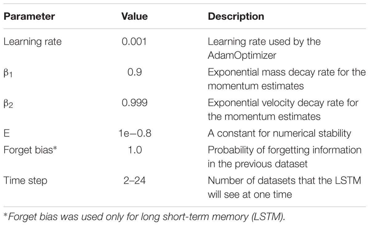
TABLE 2. Hyperparameters for recurrent neural network (RNN) and AdamOptimizer.

Data Preprocessing

Since RNNs use tangent functions and sigmoid functions internally, input data had to be normalized from 0 to 1 to improve training efficiency. In this study, RNN algorithms had the maximum time step of 72 h in environmental changes (input) and maximum output length of 24 h in EC changes (output). Both were trained after being combined into a single dataset. Data from 15 October to 24 December were randomly divided into training and validation datasets, and the rest of the data from December 25–31 were used to test the trained RNNs. Among the total datasets, 900 were used for training, 396 for validation, and 120 for test.

Results

Accuracy of the Trained Models

Among all RNN structures, an LSTM of a single layer with 64 perceptrons showed the highest accuracy (Table 3). Although the RMSE of all structures ranged from 0.08 to 0.09, the single-layered LSTM showed the highest test accuracy with R² = 0.72. Multi-layers did not improve the accuracy of RNN models. Regardless of the number of layers, LSTM showed the higher accuracy than GRU. For the same training condition, which had multi-inputs and -outputs, conventional algorithms such as ARIMA model, multivariate regression, or multi-layer perceptrons could not be trained. With the validation datasets, R² was 0.92 and RMSE was 0.07 with the LSTM (Figure 4A), which was much higher than the test accuracy with R² = 0.72 and RMSE = 0.08 (Figure 4B). Because each 24-long output was a result of one calculation, the average of each predicted and measured values was compared.

TABLE 3

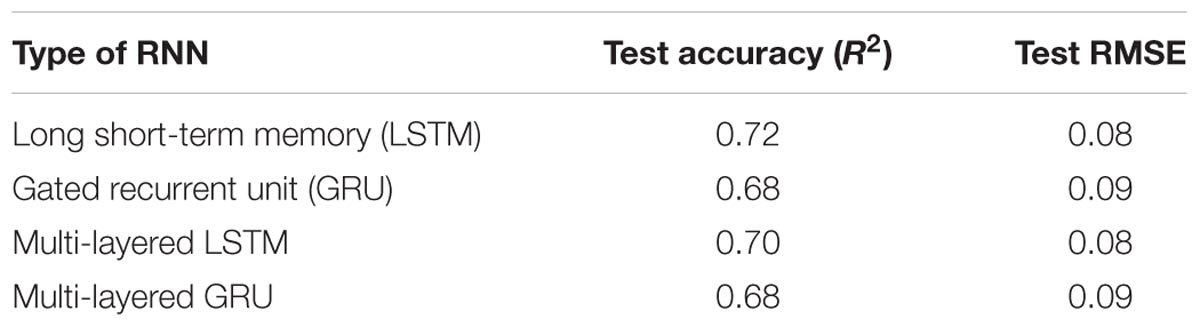
TABLE 3. Test accuracies and root mean square errors (RMSEs) of trained recurrent neural network (RNN) algorithms.

FIGURE 4

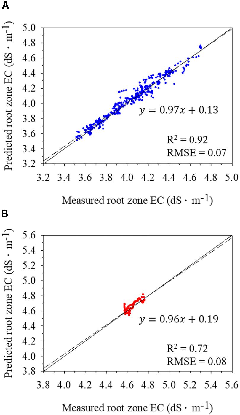
FIGURE 4. Comparisons of predicted and measured root-zone electrical conductivities (ECs) of nutrient solutions using validation (A) and test (B) datasets. Solid and dashed lines represent 1:1 line and regression line, respectively. The average of each 24-long output was presented.

Optimization of Model Parameters

The accuracy of LSTM tended to increase with extension of time step and reduction of output length. The accuracy of LSTM was highest when the time step was set to maximum. R² for the test datasets was no less than 0.65 when the time step was longer than 12 h (Figure 5A). The time step longer than 24 h did not improve the accuracy. Meanwhile, R² was lowest when output length was 24 h, but all R²s were no less than 0.72 (Figure 5B).

FIGURE 5

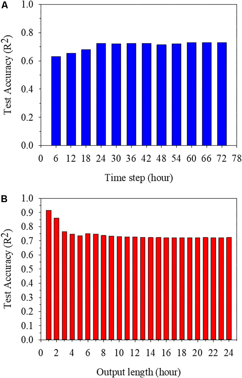
FIGURE 5. Test accuracies of trained long short-term memory (LSTM) algorithms at different time steps (A) and output lengths (B).

Among the input data, the EC of nutrient solutions in the drainage tank and cumulative irrigation volume per day most affected the substrate EC (Table 4). Both inputs reduced the test accuracy by 0.05. Substrate EC was the least influential factor in accuracy because the accuracy was rarely lowered even without substrate EC. For all inputs, the average value of reduction was 0.0295.

TABLE 4

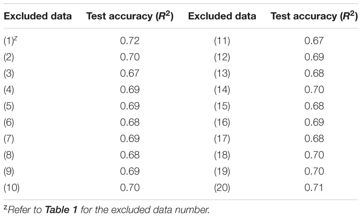
TABLE 4. Test accuracies of the long short-term memory (LSTM) after excluding input data.

Chronological Comparisons of Prediction

Trained LSTM detected the tendency and predicted the changes in EC, although there is little deviation between predicted and measured values (Figure 6). Prediction results followed the fluctuation of root-zone EC, even though variations from actual values occurred. The prediction of future 24-h EC showed different RMSEs (Figure 7). In particular, the first 3-h prediction showed lower RMSEs than the total validation RMSE. The RMSE tended to be higher in the data before 12-h, which was the beginning of the forecast. Especially, the RMSEs were lower in the first 3 h and became higher for 4–8 h. However, there was no large gap by time.

FIGURE 6

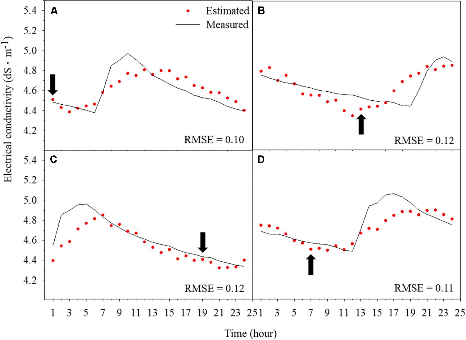
FIGURE 6. Chronological comparisons of predicted root-zone electrical conductivity (EC) via trained long short-term memory (LSTM) and measured data from 0:00 to 23:00 on December 25 (A), from 6:00 on December 26 to 5:00 on December 27 (B), from 12:00 on December 27 to 11:00 on December 28 (C), and from 18:00 on December 29 to 17:00 on December 30 (D). Arrows represent the point of 00:00.

FIGURE 7

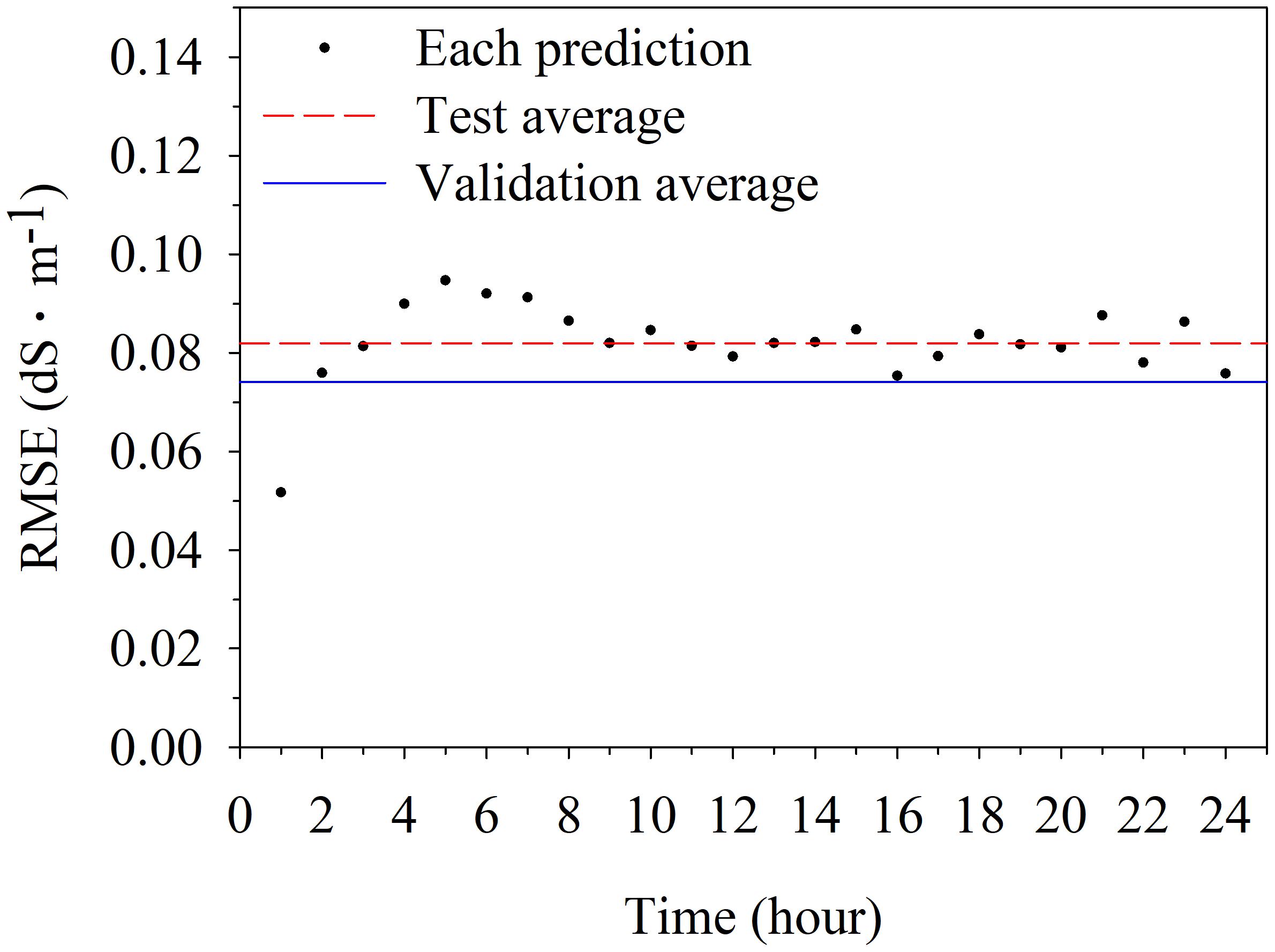
FIGURE 7. Root mean square errors (RMSEs) of electrical conductivity (EC) of nutrient solutions. RMSEs separately calculated based on each prediction for 1 h were compared with total validation and test RMSEs.

Discussion

In this study, RNN showed the test R² of 0.72, indicating that RNN had a possibility of predicting future tendency of EC changes (Figure 4). The trained RNNs with relatively shallow layers showed better accuracies in this study (Table 3). Recently, neural networks have deep structure in general (Ioffe and Szegedy, 2015; Silver et al., 2016) and RNNs have a very deep structure over time and therefore do not require fully connected multilayers in most cases (Jozefowicz et al., 2015). If the number of layers is the same, LSTM has more complex structure than GRU and has more parameters (Chung et al., 2014), resulting in higher accuracy. However, in case that the number of parameters should be small due to computational limitation, GRU can be used because the accuracy is not much different. Although ARIMA model is an algorithm to analyze chronological data, it could not predict future substrate EC. Since ARIMA model uses only target factor changes as input, it seems that the change in substrate EC itself did not show a definite periodicity. On the other hand, RNN can use other environmental factors as input, so it can correlate environmental changes with root-zone EC changes. Moreover, RNN has a unique structure and deals with huge sizes of input and output, so it is difficult to compare RNN with conventional algorithms or models.

Considering the accuracies in recent deep learning applications, the test R² of 0.72 in this study is not high and would be due to the relatively short estimation period (Figure 4). The period was a fraction of the cropping season and the data used for prediction was from 99 days after transplanting. Therefore, the earlier age of the plants could not be used because it was out of the trained ranges. However, deep learning algorithms can be more accurate when tested with big data of long periods to generalize to all possible conditions (Lopez et al., 2001). Other agricultural studies using deep learning have been conducted with big datasets with long collecting periods to cover almost all possibilities, such as seasonal influences (Trejo-Perea et al., 2009; Wang H. et al., 2017). Therefore, all datasets of other periods could improve model robustness. Adding more environmental and plant growth data to input elements can also increase the accuracy. Virtual conditions via simulation could be helpful for training the neural network (Beltramo et al., 2016). Moreover, if data are collected by similar methods used in this study, the trained LSTM can be applied to other periods or other plants using transfer learning (Gao et al., 2014; Shin et al., 2016).

EC interacts with crops and ambient environments continuously, so previous environments are related with EC changes. Therefore, the accuracy was improved with increasing time step, which represents the length of previous information (Figure 5A). However, since the nutrient solution was closed and controlled, the previous information more than 24 h did not affect the prediction accuracy. Therefore, 24-h time step is an appropriate input length. Meanwhile, the accuracy was deteriorated with increasing output lengths due to the increase in computation (Figure 5B). Obviously, the accuracy was better because the values to be predicted were reduced when the output length was shorter. However, output lengths that are too short cannot be used to help control nutrient solutions through EC forecasting. EC should be predictable from sunrise, at least when transpiration begins because transpiration and water have a significant interaction (Kramer, 1937; Greenwood and Beresford, 1979). Therefore, the maximum output length should be selected to predict the hourly changing tendency of EC in a day by using changes in environmental factors from the morning and previous day.

Through excluding input elements, it was found that the drainage nutrient solutions were highly related with the substrate EC (Table 4). However, the accuracy was not changed even if the substrate EC was eliminated from the input elements. LSTM uses the cell state to transmit the information of previous output (Greff et al., 2015; Heffernan et al., 2017). The information about the substrate EC, which is the output, could be included in the cell state. However, the accuracy was reduced by excluding water-related environments in Table 1. The changes in EC are also affected by water content (Rhoades et al., 1976; Medrano et al., 2005). Therefore, water-related data were important to predict the substrate EC. However, it can be said that all input factors were appropriate because the accuracy does not collapse by exclusion of certain factors.

The difference between accuracies resulted from generalizing the entire range of data (Figure 6). Predicting EC changes during the day was difficult because the plants disturbed the water and nutrient environments by transpiration. Underestimated or overestimated predictions between about 6 and 12 a.m. could be resulted from the increasing transpiration. In addition, transpiration significantly affects the uptake of nutrients, which is related with the change in root-zone EC and varies with growth stage (Van Noordwijk, 1990; Baille et al., 1994; Le Bot et al., 1998). Therefore, variation of the root-zone EC can be larger depending on growth stage even when the drainage rate is controlled (Massa et al., 2011; Shin and Son, 2016). In the study, the data were acquired in the latter part of the cultivation (Table 1). Since the crops were sufficiently grown, a relatively large change in the substrate EC was observed. Therefore, the trained LSTM showed a low test accuracy, but it was acceptable performance.

The RMSE showed that the trained LSTM was able to predict the entire range with even accuracy (Figure 7). Due to the nature of LSTM, which is a black box modeling, it is impossible to understand exactly what affected the RMSEs. It would not be the effect of EC change at a specific time slot because the model predicted the substrate EC at 10-min intervals. Further studies about RNN structure are needed to reveal the reason of slight differences in accuracy. However, the principle of EC-based nutrient control is maintaining the EC of nutrient solutions at a set point (Ahn et al., 2010). Therefore, predicting whether the EC will increase or decrease in the future can help with sophisticated nutrient control. Because nutrient solution control depends on a contemporary EC in current soilless cultures (Neto et al., 2014; Kinoshita et al., 2016), predicted 3-h EC might improve the accuracy of nutrient control. In addition, since the RMSE did not change much near the test accuracy of 0.08 after the 9 h, it can be said that stable forecasts during a day are possible.

Comprehensively, LSTM showed acceptable accuracies in predicting substrate EC. In addition, it is known that EC and pH can be predicted together using ANNs (Ferentinos and Albright, 2002). In this study, the pH data were not used for model training, but the pH of nutrient solution could be predicted using the LSTM. Therefore, if pH and EC can be predicted together, growers could be able to cope with rapid changes in nutrient concentration caused by environmental changes. Furthermore, LSTM, which is effective in analyzing chronological data, could predict plant environments influenced by the accumulations of previous situations, such as plant growth and ion concentration of nutrient solutions.

Conclusion

Prediction models used in this study were based on a deep learning algorithm, RNN. Among the most popular RNN algorithms, a single-layered LSTM showed the highest test accuracy (R² = 0.72). The trained LSTM could be applied to control nutrient solutions in closed-loop soilless cultures based on prediction of future EC. Therefore, the algorithm could make planned management of nutrient solutions possible, reducing resource wastes. Prediction accuracy could be higher with additional data. Deep learning algorithms could be more accurate with additional data, so other environmental factors or plant growth data could improve model robustness. In particular, the LSTM can be extended to predict various factors which are influenced by the accumulations of previous situations. Further research on long-period control using LSTM is required.

Author Contributions

TM constructed the artificial neural network, analyzed the root-zone EC, and wrote the manuscript. TIA developed the open-loop soilless culture system and measured the environment and growth data. JES designed and supervised the experiment and wrote the manuscript.

Funding

This research was supported by the MSIT (Ministry of Science and ICT), Korea, under the ITRC (Information Technology Research Center) support program (IITP-2017-2013-0-00877) supervised by the IITP (Institute for Information and Communications Technology Promotion).

Conflict of Interest Statement

The authors declare that the research was conducted in the absence of any commercial or financial relationships that could be construed as a potential conflict of interest.

The reviewer AC and the handling editor declared their shared affiliation.

References

Adavanne, S., Pertilä, P., and Virtanen, T. (2017). Sound event detection using spatial features and convolutional recurrent neural network. arXiv:1706.02291 [Preprint].

Ahn, T. I., Shin, J. W., and Son, J. E. (2010). Analysis of changes in ion concentration with time and drainage ratio under EC-based nutrient control in closed-loop soilless culture for sweet pepper plants (Capsicum annum L.’Boogie’). J. Bioenviron. Cont. 19, 298–304.

Google Scholar

Baille, M., Baille, A., and Laury, J. C. (1994). A simplified model for predicting evapotranspiration rate of nine ornamental species vs. climate factors and leaf area. Sci. Hortic. 59, 217–232. doi: 10.1016/0304-4238(94)90015-9

CrossRef Full Text | Google Scholar

Beltramo, T., Ranzan, C., Hinrichs, J., and Hitzmann, B. (2016). Artificial neural network prediction of the biogas flow rate optimised with an ant colony algorithm. Biosyst. Eng. 143, 68–78. doi: 10.1016/j.biosystemseng.2016.01.006

CrossRef Full Text | Google Scholar

Cho, K., van Merriënboer, B., Gulcehre, C., Bahdanau, D., Bougares, F., Schwenk, H., et al. (2014). Learning phrase representations using RNN encoder-decoder for statistical machine translation. arXiv:1406.1078 [Preprint]. doi: 10.3115/v1/d14-1179

CrossRef Full Text

Chung, J., Gulcehre, C., Cho, K., and Bengio, Y. (2014). Empirical evaluation of gated recurrent neural networks on sequence modeling. arXiv:1412.3555 [Preprint].

Dewir, Y. H., Chakrabarty, D., Ali, M. B., Hahn, E. J., and Paek, K. Y. (2005). Effects of hydroponic solution EC, substrates, PPF and nutrient scheduling on growth and photosynthetic competence during acclimatization of micropropagated Spathiphyllum plantlets. Plant Growth Regul. 46, 241–251. doi: 10.1007/s10725-005-0161-1

CrossRef Full Text | Google Scholar

Draeger, A., Engell, S., and Ranke, H. (1995). Model predictive control using neural networks. IEEE Control Syst. 15, 61–66. doi: 10.1109/37.466261

CrossRef Full Text | Google Scholar

Esfe, M. H., Ahangar, M. R. H., Rejvani, M., Toghraie, D., and Hajmohammad, M. H. (2016). Designing an artificial neural network to predict dynamic viscosity of aqueous nanofluid of TiO2 using experimental data. Int. J. Heat Mass Transf. 75, 192–196. doi: 10.1016/j.icheatmasstransfer.2016.04.002

CrossRef Full Text | Google Scholar

Fargašová, A. (1994). Effect of Pb, Cd, Hg, As, and Cr on germination and root growth of Sinapis alba seeds. Bull. Environ. Contam. Toxicol. 52, 452–456. doi: 10.1007/BF00197836

PubMed Abstract | CrossRef Full Text | Google Scholar

Ferentinos, K. P., and Albright, L. D. (2002). Predictive neural network modeling of pH and electrical conductivity in deep–trough hydroponics. Trans. ASAE 45:007. doi: 10.13031/2013.11412

CrossRef Full Text | Google Scholar

Gao, J., Ling, H., Hu, W., and Xing, J. (2014). “Transfer learning based visual tracking with gaussian processes regression,” in Proceedings of the European Conference on Computer Vision, eds D. Fleet, T. Pajdla, B. Schiele, and T. Tuytelaars (Zurich: Springer), 188–203. doi: 10.1007/978-3-319-10578-9_13

CrossRef Full Text | Google Scholar

Greenwood, E. A. N., and Beresford, J. D. (1979). Evaporation from vegetation in landscapes developing secondary salinity using the ventilated-chamber technique: I. Comparative transpiration from juvenile Eucalyptus above saline groundwater seeps. J. Hydrol. 42, 369–382. doi: 10.1016/0022-1694(79)90056-8

CrossRef Full Text | Google Scholar

Greff, K., Srivastava, R. K., Koutník, J., Steunebrink, B. R., and Schmidhuber, J. (2015). LSTM: a search space odyssey. arXiv:1503.04069 [Preprint]. doi: 10.1109/tnnls.2016.2582924

PubMed Abstract | CrossRef Full Text

Griffin, B. A., and Jurinak, J. J. (1973). Estimation of activity coefficients from the electrical conductivity of natural aquatic systems and soil extracts. Soil Sci. 116, 26–30. doi: 10.1097/00010694-197307000-00005

CrossRef Full Text | Google Scholar

Heffernan, R., Yang, Y., Paliwal, K., and Zhou, Y. (2017). Capturing non-local interactions by long short-term memory bidirectional recurrent neural networks for improving prediction of protein secondary structure, backbone angles, contact numbers and solvent accessibility. Bioinformatics 33, 2842–2849. doi: 10.1093/bioinformatics/btx218

PubMed Abstract | CrossRef Full Text | Google Scholar

Hochreiter, S., and Schmidhuber, J. (1997). Long short-term memory. Neural Comput. 9, 1735–1780. doi: 10.1162/neco.1997.9.8.1735

CrossRef Full Text | Google Scholar

Ioffe, S., and Szegedy, C. (2015). Batch normalization: accelerating deep network training by reducing internal covariate shift. arXiv:1502.03167 [Preprint].

Jovicich, E., Cantliffe, D. J., and Stoffella, P. J. (2004). Fruit yield and quality of greenhouse-grown bell pepper as influenced by density, container, and trellis system. HortTechnology 14, 507–513.

Google Scholar

Jozefowicz, R., Zaremba, W., and Sutskever, I. (2015). “An empirical exploration of recurrent network architectures,” in Proceedings of the 32nd International Conference on Machine Learning, eds F. Bach and D. Blei, Lille, 2342–2350. Available at: http://proceedings.mlr.press/v37/ jozefowicz15.pdf

Google Scholar

Kingma, D. P., and Ba, J. (2014). Adam: a method for stochastic optimization. arXiv:1412.6980v9 [Preprint].

Kinoshita, T., Yamazaki, H., Inamoto, K., and Yamazaki, H. (2016). Analysis of yield components and dry matter production in a simplified soilless tomato culture system by using controlled-release fertilizers during summer–winter greenhouse production. Sci. Hortic. 202, 17–24. doi: 10.1016/j.scienta.2016.02.019

CrossRef Full Text | Google Scholar

Kramer, P. J. (1937). The relation between rate of transpiration and rate of absorption of water in plants. Am. J. Bot. 24, 10–15. doi: 10.2307/2436949

CrossRef Full Text | Google Scholar

Ku, C. S., and Hershey, D. R. (1991). Leachate electrical conductivity and growth of potted poinsettia with leaching fractions of 0 to 0.4. J. Am. Soc. Hortic. Sci. 116, 802–806.

Google Scholar

Le Bot, J., Adamowicz, S., and Robin, P. (1998). Modelling plant nutrition of horticultural crops: a review. Sci. Hortic. 74, 47–82. doi: 10.1016/S0304-4238(98)00082-X

CrossRef Full Text | Google Scholar

Le Bot, J., Jeannequin, B., and Fabre, R. (2001). Impacts of N-deprivation on the yield and nitrogen budget of rockwool grown tomatoes. Agronomie 21, 341–350. doi: 10.1051/agro:2001128

CrossRef Full Text | Google Scholar

LeCun, Y., Bengio, Y., and Hinton, G. (2015). Deep learning. Nature 521, 436–444. doi: 10.1038/nature14539

PubMed Abstract | CrossRef Full Text | Google Scholar

Lopez, G., Rubio, M. A., Martınez, M., and Batlles, F. J. (2001). Estimation of hourly global photosynthetically active radiation using artificial neural network models. Agric. For. Meteorol. 107, 279–291. doi: 10.1016/s0168-1923(01)00217-9

PubMed Abstract | CrossRef Full Text | Google Scholar

Lykas, C., Katsoulas, N., Giaglaras, P., and Kittas, C. (2006). Electrical conductivity and pH prediction in a recirculated nutrient solution of a greenhouse soilless rose crop. J. Plant Nutr. 29, 1585–1599. doi: 10.1080/01904160600848904

CrossRef Full Text | Google Scholar

Massa, D., Incrocci, L., Maggini, R., Bibbiani, C., Carmassi, G., Malorgio, F., et al. (2011). Simulation of crop water and mineral relations in greenhouse soilless culture. Environ. Modell. Softw. 26, 711–722. doi: 10.1016/j.envsoft.2011.01.004

CrossRef Full Text | Google Scholar

Medrano, E., Lorenzo, P., Sánchez-Guerrero, M. C., and Montero, J. I. (2005). Evaluation and modelling of greenhouse cucumber-crop transpiration under high and low radiation conditions. Sci. Hortic. 105, 163–175. doi: 10.1016/j.scienta.2005.01.024

CrossRef Full Text | Google Scholar

Mnih, V., Kavukcuoglu, K., Silver, D., Rusu, A. A., Veness, J., Bellemare, M. G., et al. (2015). Human-level control through deep reinforcement learning. Nature 518, 529–533. doi: 10.1038/nature14236

PubMed Abstract | CrossRef Full Text | Google Scholar

Neto, A. J. S., Zolnier, S., and de Carvalho Lopes, D. (2014). Development and evaluation of an automated system for fertigation control in soilless tomato production. Comput. Electron. Agric. 103, 17–25. doi: 10.1016/j.compag.2014.02.001

CrossRef Full Text | Google Scholar

Nicoletto, C., Maucieri, C., and Sambo, P. (2017). Effects on water management and quality characteristics of ozone application in chicory forcing process: a pilot system. Agronomy 7:29. doi: 10.3390/agronomy7020029

CrossRef Full Text | Google Scholar

Ororbia, I. I., Alexander, G., Mikolov, T., and Reitter, D. (2017). Learning simpler language models with the delta recurrent neural network framework. arXiv:1703.08864 [Preprint]. doi: 10.1162/neco_a_01017

PubMed Abstract | CrossRef Full Text

Rhoades, J. D., Raats, P. A. C., and Prather, R. J. (1976). Effects of liquid-phase electrical conductivity, water content, and surface conductivity on bulk soil electrical conductivity 1. Soil Sci. Soc. Am. J. 40, 651–655. doi: 10.2136/sssaj1976.03615995004000050017x

CrossRef Full Text | Google Scholar

Rumelhart, D. E., Hinton, G. E., and Williams, R. J. (1988). Learning representations by back-propagating errors. Cogn. Model. 5:1. doi: 10.1038/323533a0

CrossRef Full Text | Google Scholar

Savvas, D. (2002). SW—Soil and Water: automated replenishment of recycled greenhouse effluents with individual nutrients in hydroponics by means of two alternative models. Biosyst. Eng. 83, 225–236. doi: 10.1006/bioe.2002.0106

CrossRef Full Text | Google Scholar

Savvas, D., and Manos, G. (1999). Automated composition control of nutrient solution in closed soilless culture systems. J. Agric. Eng. Res. 73, 29–33. doi: 10.1006/jaer.1998.0389

CrossRef Full Text | Google Scholar

Shin, H. C., Roth, H. R., Gao, M., Lu, L., Xu, Z., Nogues, I., et al. (2016). Deep convolutional neural networks for computer-aided detection: CNN architectures, dataset characteristics and transfer learning. IEEE Trans. Med. Imaging 35, 1285–1298. doi: 10.1109/TMI.2016.2528162

PubMed Abstract | CrossRef Full Text | Google Scholar

Shin, J. H., and Son, J. E. (2016). Application of a modified irrigation method using compensated radiation integral, substrate moisture content, and electrical conductivity for soilless cultures of paprika. Sci. Hortic. 198, 170–175. doi: 10.1016/j.scienta.2015.11.015

CrossRef Full Text | Google Scholar

Siddiqi, M. Y., Kronzucker, H. J., Britto, D. T., and Glass, A. D. M. (1998). Growth of a tomato crop at reduced nutrient concentrations as a strategy to limit eutrophication. J. Plant Nutr. 21, 1879–1895. doi: 10.1080/01904169809365530

CrossRef Full Text | Google Scholar

Silver, D., Huang, A., Maddison, C. J., Guez, A., Sifre, L., Van Den Driessche, G., et al. (2016). Mastering the game of Go with deep neural networks and tree search. Nature 529, 484–489. doi: 10.1038/nature16961

PubMed Abstract | CrossRef Full Text | Google Scholar

Sonneveld, C., and Voogt, W. (2009). “Nutrient management in substrate systems,” in Proceedings of the Plant Nutrition of Greenhouse Crops, eds K. D. K. Sturm and F. Stampar (Dordrecht: Springer), 277–312. doi: 10.1007/978-90-481-2532-6_13

CrossRef Full Text | Google Scholar

Stutte, G. W. (2006). Process and product: recirculating hydroponics and bioactive compounds in a controlled environment. HortScience 41, 526–530.

Google Scholar

Trejo-Perea, M., Herrera-Ruiz, G., Rios-Moreno, J., Miranda, R. C., and Rivasaraiza, E. (2009). Greenhouse energy consumption prediction using neural networks models. Int. J. Agric. Biol. 11, 1–6. doi: 10.1007/s11356-017-9216-x

PubMed Abstract | CrossRef Full Text | Google Scholar

Van Noordwijk, M. (1990). “Synchronisation of supply and demand is necessary to increase efficiency of nutrient use in soilless horticulture,” in Plant Nutrition—Physiology and Applications (Dordrecht: Springer), 525–531. doi: 10.1007/978-94-009-0585-6_87

CrossRef Full Text | Google Scholar

Wang, F., Xiang, X., Liu, C., Tran, T. D., Reiter, A., Hager, G. D., et al. (2017). Transferring face verification nets to pain and expression regression. arXiv:1702.06925 [Preprint].

Wang, H., Sánchez-Molina, J. A., Li, M., Berenguel, M., Yang, X. T., and Bienvenido, J. F. (2017). Leaf area index estimation for a greenhouse transpiration model using external climate conditions based on genetics algorithms, back-propagation neural networks and nonlinear autoregressive exogenous models. Agric. Water Manage 183, 107–115. doi: 10.1016/j.agwat.2016.11.021

CrossRef Full Text | Google Scholar