Effects of extracellular metabolic acidosis on the homeostasis of intracellular pH in hippocampal neurons

This Hypothesis & Theory contribution accompanies the research paper by Bouyer et al. (Frontiers in Physiology 2024), the first to employ out-of-equilibrium (OOE) CO₂/HCO₃⁻ solutions to examine systematically the intracellular pH (pH_i) effects of extracellular (o) metabolic acidosis (MAc) and its components: an isolated decrease in pH_o (pure acidosis, pAc) and an isolated decrease in [HCO₃⁻]_o (pure metabolic/down, pMet↓). In this study, after reviewing various types of acid–base disturbances and the use of OOE solutions, we discuss pH_i “state” (ΔpH_i, in response to a single acid–base challenge) and “behavior” (the ΔpH_i transition observed between two successive challenges), along with approaches for quantifying state and behavior. We then discuss the molecular basis of how individual extracellular acid–base disturbances influence pH_i via effects on—and interactions among—acid–base transporters, acid–base sensors, and cellular constitution. Next, we examine the determinants of states and behaviors, their impact on the buffering of extracellular acid loads, and how variability in state and behavior might arise. We conclude with a consideration of how mathematical models—despite their inherent limitations—might assist in the interpretation of experiments and qualitative models presented in this study. Among the themes that emerge are (1) hippocampal neurons must have distinct sensors for pH_o and [HCO₃⁻]_o; (2) these pH_o- and [HCO₃⁻]_o-driven signal transduction pathways produce additive pH_i effects in naïve neurons (those not previously challenged by an acid–base disturbance); and (3) these pathways produce highly non-additive pH_i effects in neurons previously challenged by MAc.

Introduction

Virtually, all biological processes—including those of the central nervous system—are sensitive to changes in pH. Mammals regulate the pH of the blood and extracellular fluid by adjusting the ratio of the two members of the key buffer pair: CO₂ and HCO₃⁻. The lungs control [CO₂] by altering ventilation. The kidneys control [HCO₃⁻] by altering the rate at which they secrete H⁺ into the tubule fluid and simultaneously move HCO₃⁻ into the blood.

The acid–base status of the blood and extracellular fluid has a major influence on the pH inside the cells. Thus, we expect factors that disturb the extracellular [CO₂]/[HCO₃⁻] ratio to influence the acid–base status of cells, as discussed by Bouyer et al. (2024). Conversely, as cells attempt to stabilize their own pH, they move acid–base equivalents across the plasma membrane, thereby disrupting the acid–base status of the extracellular fluid.

A recent paper by Bouyer et al. (2024) explored how one particular extracellular acid–base disturbance, termed metabolic acidosis, affects the pH of rat hippocampal (HC) neurons in primary culture. As discussed in the following sections, metabolic acidosis involves a decrease in both extracellular pH and [HCO₃⁻]. Bouyer and his colleagues used techniques to independently lower each of these parameters and, in the process, made several interesting—and in one case, startling—observations about how single and successive bouts of metabolic acidosis (or its components) affect neuronal pH_i.

The purposes of this Hypothesis and Theory contribution are twofold: (1) to provide the readers of the Bouyer paper with some background for understanding the reported findings and (2) to offer potential explanations for the sometimes unexpected observations. Note that the general principles introduced in this study—for single rat HC neurons in the Bouyer paper—ought to apply to any individual eukaryotic cell, including those that are part of more complex systems such as neuron–glial co-cultures, brain slices, intact brains, diverse epithelia, and even more complex tissues like the renal cortex and blood–brain barrier. Each cell type (including different types of neurons) may require a unique set of parameters to account for their pH_i homeostatic mechanisms. Moreover, complex structures likely call for unique forms of cell–cell communication and, thus, control over transporters and sensors.

Acid–base disturbances

Metabolic acidosis (MAc) is a common and potentially life-threatening acid–base disorder in mammals, including humans. It is caused by a depletion of extracellular (o) HCO₃⁻, which leads to a decrease in both [HCO₃⁻]_o and pH_o. In a living animal, MAc generally triggers a compensatory increase in ventilation, which lowers [CO₂]_o and thereby mitigates the decrease in pH_o. Under these conditions, all three fundamental CO₂/HCO₃⁻ acid–base parameters underwent changes, making it difficult to attribute the effects of compensated MAc to decreased [HCO₃⁻]_o, decreased pH_o, or decreased [CO₂]_o—or some combination of the three.

In vitro, we can equilibrate artificial solutions with a known partial pressure of CO₂, thereby preventing changes in [CO₂]_o. Even under these conditions, however, MAc is usually associated with two altered parameters—a decrease in [HCO₃⁻]_o and a decrease in pH_o—therefore, it is still difficult to know whether the effects of MAc are due to the reduction in [HCO₃⁻]_o per se or pH_o per se.

In addition to MAc, the three other fundamental acid–base disturbances (see Boron, 2017) are metabolic alkalosis (MAlk), in which an increase in [HCO₃⁻]_o causes pH_o to increase; respiratory acidosis (RAc), in which an increase in [CO₂]_o causes pH_o to decrease; and respiratory alkalosis (RAlk), in which a decrease in [CO₂]_o causes pH_o to increase. In all of these cases, the disturbance in an intact animal leads to changes in all three acid–base parameters, along the lines discussed in the first paragraph. In the laboratory, it is possible—under equilibrium conditions—to change two at a time.

A breakthrough occurred in 1995 with the development of a rapid-mixing approach for generating out-of-equilibrium (OOE) CO₂/HCO₃⁻ solutions (Zhao et al., 1995), which—over a wide range of pH values—can have any combination of [CO₂]_o, [HCO₃⁻]_o, and pH_o.

The use of OOE solutions offers a promising approacht o determining the extent to which individual acid–base parameters contribute to the physiological effects of MAc. The first such study was by Zhao et al. (2003), who found—on a background of a normal CO₂/HCO₃⁻ solution—that the isolated removal of basolateral (BL; i.e., blood-side) HCO₃⁻ from isolated, perfused proximal tubules (PTs)—leaving [CO₂]_BL and pH_BL unchanged—caused the rate of transepithelial HCO₃⁻ reabsorption (J_HCO3), measured over ∼20 min, to increase. Thus, this challenge—the most extreme possible example of MAc but without acidosis—produced the appropriate compensatory response.

Extending the work of Zhao and her coworkers, Zhou et al. (2005) used OOE solutions in a study in which they systematically varied [CO₂]_BL between 0% and 20% (leaving [HCO₃⁻]_BL and pH_BL fixed), varied [HCO⁻₃]_BL from 0 mM to 44 mM (leaving [CO₂]_BL and pH_BL fixed), or varied pH_BL from 6.8 to 8.0 (leaving [CO₂]_BL and [HCO⁻₃]_BL fixed). Surprisingly, they found that acute¹ changes in pH_BL had no effect on J_HCO3 over the ∼20-min duration of the challenges. However, starting at conditions that mimicked the composition of normal arterial blood—[CO₂]_o = 5%, [HCO₃⁻]_o = 22 mM; pH_o = 7.40—isolated changes in [CO₂]_o or [HCO₃⁻]_o produced the appropriate compensatory effects:

(1) Isolated decrease in [HCO₃⁻]_o ([CO₂]_o and pH_o constant). Bouyer et al. (2024) named this disturbance “pure metabolic/down (pMet↓).” It is the metabolic part of MAc but without acidosis. Both Zhao et al. (2003) and Zhou et al. (2005) found that pMet↓ caused J_HCO3 to increase, which would tend to compensate for MAc.

(2) Isolated increase in [HCO₃⁻]_o ([CO₂]_o and pH_o constant). Bouyer et al. (2024) introduced the term “pure metabolic/up (pMet↑)” in their nomenclature to describe this disturbance. It is the metabolic part of MAlk but without alkalosis. Zhou et al. (2005) found that pMet↑ caused J_HCO3 to decrease, which would tend to compensate for MAlk.

(3) Isolated increase in [CO₂]_o ([HCO₃⁻]_o and pH_o constant). Bouyer et al. (2024) did not propose a name for this disturbance, but we suggest “pure respiratory/up (pResp↑),” where we understand the arrow as pertaining to [CO₂]_o. It is the respiratory part of RAc but without acidosis. Zhou et al. (2005) found that pResp↑ caused J_HCO3 to increase, which would tend to compensate for RAc.

(4) Isolated decrease in [CO₂]_o ([HCO₃⁻]_o and pH_o constant). Bouyer et al. (2024) did not propose a name for this disturbance, but we suggest “pure respiratory/down (pResp↓),” where we again understand the arrow as pertaining to [CO₂]_o. It is the respiratory part of RAlk but without alkalosis. Both Zhao et al. (2003) and Zhou et al. (2005) found that pResp↓ caused J_HCO3 to decrease, which would tend to compensate for RAlk.

In a somewhat different protocol, Bouyer et al. (2003) started with a rabbit PT exposed on both the apical (i.e., lumen) and basolateral sides to a CO₂/HCO₃⁻-free solution. Adding equilibrated CO₂/HCO₃⁻ to the basolateral side caused a rapid increase in [Ca²⁺]_i, whereas adding CO₂/HCO₃⁻ to the lumen had no effect on [Ca²⁺]_i. Switching to an OOE basolateral solution that contained physiological CO₂ but not HCO₃⁻ (“pure CO₂”) replicated the increase in [Ca²⁺]_i, whereas switching to an OOE basolateral solution that contained physiological HCO₃⁻ but not CO₂ (“pure HCO₃⁻”) had little effect on [Ca²⁺]_i. Thus, it may be that it is basolateral CO₂—in part acting through Ca²⁺—that triggers an increase in J_HCO3 in PTs. With our current knowledge of receptor protein tyrosine phosphatase γ (RPTPγ), we would now hypothesize that—if we started with equilibrated CO₂/HCO₃⁻ in the luminal and basolateral solutions—an isolated decrease in [HCO₃⁻]_o would have the same effect on [Ca²⁺]_i as would increasing [CO₂]_o.

The results of Zhao et al. (2003), Bouyer et al. (2003), and Zhou et al. (2005) were the first to unequivocally demonstrate that, independent of pH, each of the two components of the major blood buffer—CO₂ and HCO₃⁻—can act as acute, potent modulators of a biological function.

Neuronal pH_i homeostasis in the face of metabolic acidosis

In an earlier study of cultured rat neurons, Bouyer and colleagues (2004) examined the effects of all four fundamental acid–base disturbances on the pH_i of both medullary-raphé (MR) neurons and HC neurons. For MAlk, RAc, and RAlk (but not MAc), both MR and HC neurons exhibited fully reversible pH_i changes, with ΔpH_i/ΔpH_o ratios of ∼60%. For MAc, the responses were more intriguing. Although most MR neurons and some HC neurons exhibited a ΔpH_i/ΔpH_o of ∼65%, some MR neurons and most HC neurons exhibited a ΔpH_i/ΔpH_o of only ∼9% (Bouyer et al., 2004). Later, Salameh and colleagues (2014) coined the terms “MAc-sensitive” and “MAc-resistant” to describe cells like those reported by Bouyer in response to a single acid–base challenge. Interestingly, and apropos of the most recent paper by Bouyer et al. (2024), Bouyer’s 2004 neurons that we would now term MAc-resistant, when switched from a MAc solution to a control solution, they often exhibited a pH_i rebound to a value above the initial baseline pH_i. A theoretical analysis led Bouyer et al. (2004) to hypothesize that the MAc-resistant neurons have a sensor for extracellular HCO₃⁻ and that a decrease in [HCO₃⁻]_o triggers an immediate stimulation of neuronal acid–base transporters that minimizes the MAc-induced decrease in pH_i.

Salameh et al. (2014), based on observed MAc-induced pH_i changes in 10 cell types, proposed that the demarcation between MAc-resistant and MAc-sensitive is a (ΔpH_i)/(ΔpH_o) of 40%. They pointed out that any such quantitative criterion is somewhat arbitrary.

Salameh et al. (2014) also extended the protocol of Bouyer et al. (2004) by including two successive MAc challenges, MAc₁ and MAc₂, separated by a period of recovery in a control CO₂/HCO₃⁻ solution. Comparing the pH_i induced by MAc₂ vs. MAc₁, they categorized neurons as “adapting” to the MAc challenge when ΔpH_i during MAc₂—(ΔpH_i)_2/MAc—was sufficiently smaller in magnitude than (ΔpH_i)_1/MAc, being “consistent” if the two ΔpH_i values were reasonably close and “decompensating” if the magnitude of (ΔpH_i)_2/MAc was sufficiently greater than that of (ΔpH_i)_1/MAc.

In their recent paper, Bouyer et al. (2024) expanded upon previous work by examining substitutions of pAc or pMet↓ for MAc in HC rat neurons in primary culture. They referred to resistance and sensitivity as two relative “states” of neurons, defined for single challenges (e.g., MAc₁ and MAc₂). They also referred to adaptation, consistency, and decompensation, defined for the transition from the first to the second challenge, as three “behaviors.”

In her PhD dissertation, Taki (2024) examined the twin challenges of MAc and RAc in murine co-cultures of HC neurons and astrocytes. Analyzing their data along the lines of Bouyer et al. (2024), Taki et al. found that the global knockout of RPTPζ, a candidate sensor of [CO₂]_o and [HCO₃⁻]_o expressed mainly in the central nervous system (CNS), led to much larger acidifications than those observed in cells from WT mice.

In the following sections², we provide a more formal presentation of state and behavior, along with methods for assessing them.

Out-of-equilibrium solutions

“The basics”

In the paper by Bouyer et al. (2024), the major contribution is the use of OOE solutions to dissect the contributions of the two components of MAc: the decreased pH_o per se and the decreased [HCO₃⁻]_o per se. The key to understanding OOE technology is the fact that the interconversion between CO₂ and H₂O, on one hand, and H⁺ and HCO₃⁻, on the other hand, involves two reactions, one of which is very slow and the other is very fast. The OOE approach separates chemical species on opposite sides of the slow reaction in the following sequence:

${\text{CO}}_2+{\mathrm{H}}_2\mathrm{O}\stackrel{slow}{\rightleftharpoons }{\mathrm{H}}_2{\text{CO}}_3\stackrel{fast}{\rightleftharpoons }{\mathrm{H}}^{+}+{\text{HCO}}_3^{-}.(1)$

Although we can independently control [CO₂]_o, [H⁺]_o (i.e., pH_o), and [HCO₃⁻]_o per se, we have less influence over other chemical species that depend directly or indirectly on any of the entities in the preceding two-step reaction. An important example is [CO₃⁼]_o, which depends on both [H⁺]_o and [HCO₃⁻]_o:

${\text{HCO}}_3^{-}\rightleftharpoons {\mathrm{H}}^{+}+{\text{CO}}_3^{=}.(2)$

Moreover, the concentration of the NaCO₃⁻ ion pair depends on both [Na⁺]_o and [CO₃⁼]_o (as in Equation 3):

${\text{Na}}^{+}+{\text{CO}}_3^{=}\rightleftharpoons {\text{NaCO}}_3^{-},(3)$

${\text{CO}}_3^{=}$ and NaCO₃⁻ are important for pH_i homeostasis because they are potential substrates of Na⁺-coupled HCO₃⁻ transporters as our group suggested in the 1980s and 1990s (Boron and Boulpaep, 1983; Boron and Russell, 1983; Boron, 1985; Boron and Knakal, 1989; 1992). A combination of electrophysiological and mathematical modeling approaches now shows that either Na⁺ + CO₃⁼ or NaCO₃⁻ is the actual substrate of both the electrogenic Na/HCO₃ cotransporter NBCe1 and the Na⁺-driven Cl-HCO₃ exchanger NDCBE (Lee et al., 2023). Because both transporters—and closely related members of the “solute-linked carrier” 4 (SLC4) family—play important roles in pH_i regulation of both neurons and astrocytes, it is instructive to consider how our experimental challenges impact [CO₃⁼]_o.

If we assume for a moment that the second reaction in Equation 1 is infinitely slow—and if the reaction sequence in Equation 1 represents the only significant pathway between CO₂/H₂O and H⁺/HCO₃⁻—then it is easy to observe how we could control [CO₂] independently of [H⁺] and [HCO₃⁻] and vice versa. The “slow” reaction in Equation 1 is slow enough that we can exploit it to make OOE solutions. The principle behind the OOE approach is to mix, with sufficient speed, two dissimilar CO₂/HCO₃⁻/pH solutions.

Other reactions and considerations

In addition to the reactions shown in Equation 1, which is typically the pathway shown in textbooks (see Boron, 2017), a parallel mechanism also converts CO₂ to HCO₃⁻:

$\underset{0.0012\mathrm{M}}{\underbrace{{\text{CO}}_2}}+\underset{3.16\times {10}^{-7}\mathrm{M}}{\underbrace{{\text{OH}}^{-}}}{\displaystyle \underset{25{}^{\mathrm{o}}\mathrm{C}}{\stackrel{k_1=4\times {10}^3\mathrm{L}\cdot {\text{mol}}^{-1}\cdot {\mathrm{s}}^{-1}}{\to }}}{\text{HCO}}_3^{-}.(4)$

The concentration values below the braces approximately correspond to a physiological partial pressure of CO₂ (P_CO2) and a pH value of 7.5 at 25°C. Multiplying these concentration values by the forward rate constant yields a reaction velocity of

$v_{{\text{CO}}_2+{\text{OH}}^{-}}=\left(4\times {10}^3\mathrm{L}\cdot {\text{mol}}^{-1}\cdot {\mathrm{s}}^{-1}\right)\times \left(1.2\times {10}^{-3}\text{\hspace{0.17em}mol}\cdot {\mathrm{L}}^{-1}\right)\times \left(3.16\times {10}^{-7}\text{mol}\cdot {\mathrm{L}}^{-1}\right)$

$\cong 1.5\times {10}^{-6}\mathrm{M}\cdot {\mathrm{s}}^{-1}=1.5\times {10}^{-3}\text{mM}\cdot {\mathrm{s}}^{-1}.(5)$

In the case of the first reaction in Equation 1,

$\underset{0.0012\mathrm{M}}{\underbrace{{\text{CO}}_2}}+{\mathrm{H}}_2\mathrm{O}{\displaystyle \underset{25{}^{\mathrm{o}}\mathrm{C}}{\stackrel{k_1=0.036{\mathrm{s}}^{-1}}{\to }}}{\mathrm{H}}_2{\text{CO}}_3,(6)$

the forward rate constant predicts a reaction rate of

$v_{{\text{CO}}_2+{\mathrm{H}}_2\mathrm{O}}=\left(3.6\times {10}^{-2}{\mathrm{s}}^{-1}\right)\times \left(1.2\times {10}^{-3}\text{\hspace{0.17em}mol}\cdot {\mathrm{L}}^{-1}\right)$

$\cong 4.3\times {10}^{-5}\mathrm{M}\cdot {\mathrm{s}}^{-1}=4.3\times {10}^{-2}\text{mM}\cdot {\mathrm{s}}^{-1}.(7)$

H₂CO₃, the product of the “CO₂ + H₂O” reaction in Equation 6, would rapidly break down to form H⁺ and HCO₃⁻. Thus, it is reasonable to compare the velocity (Equation 7) of the “CO₂ + H₂O″ reaction in Equation 6 with that of the “CO₂ + OH⁻” reaction in Equation 4, which is only ∼3.5% as fast (Equation 5). This is why the OH⁻reaction in Equation 4 is generally ignored at physiological blood pH. However, the OH⁻pathway in Equation 4 is strikingly pH-sensitive because as pH increases, [OH⁻] increases exponentially. Thus, at a pH value of 9.0, the velocity of the “CO₂ + OH⁻” reaction in Equation 4 is already 11% greater than that of the “CO₂ + H₂O” reaction in Equation 6. At pH 10.0, it is 11-fold faster and so on.

The pH sensitivity of the OH⁻reaction has important implications for generating OOE solutions. Imagine that you wanted to generate a “pure CO₂ solution,” one with a physiological [CO₂] but almost no HCO₃⁻ at pH 7.4. You might be inclined to mix a CO₂ solution at low pH (e.g., 5.4, where most of the carbon would be in the form of CO₂) with a CO₂/HCO₃⁻-free solution at a very high pH (e.g., 10). However, you will find that your final [CO₂] will be much lower than expected, whereas your final [HCO₃⁻] will be much higher. The reason, it seems, is that the macroscopic mixing process described in Figure 1 initially generates microdomains that contain unmixed versions of the acidic/high-CO₂ solution and the very alkaline solution. At the interface, the reaction CO₂ + OH⁻ → HCO₃⁻ unexpectedly consumes your CO₂ and disrupts your anticipated near-HCO₃⁻-free state.

Figure 1

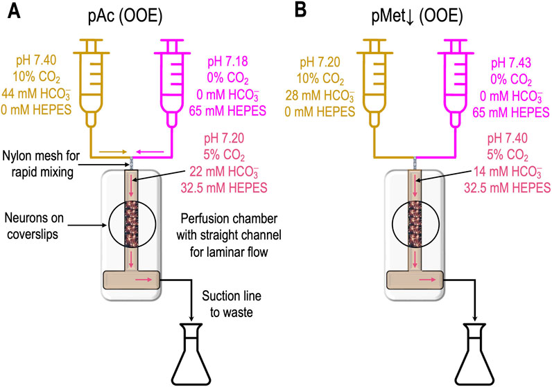
Figure 1. Generation of out-of-equilibrium solutions (A). A heavy-duty dual syringe pump drives (at identical rates) two syringes, the acid–base contents of which are summarized by the gold-colored and magenta labels. The blended gold/magenta labels indicate the composition of the solution at the instant of mixing. The continuously generated OOE solution flows past the neurons in the chamber, before being discarded into a waste receptacle and then suctioned into an external waste container. (B) Generation of a pure metabolic/down (pMet↓) solution. The approach is the same as in panel A except for the contents of the two syringes.

Another reaction can also wreak havoc with the creation of OOE solutions. Assume that you wanted to generate a “pure HCO₃⁻” solution, one with a physiological [HCO₃⁻] but almost no CO₂ at pH 7.4. You might be inclined to mix an HCO₃⁻ solution at a high pH value (e.g., 9.4, where most of the carbon would be in the form of HCO₃⁻ and CO₃⁼) with a CO₂/HCO₃⁻-free solution at a very low pH value (e.g., 5). However, you will find that your final [HCO₃⁻] will be much lower than expected, whereas your final [CO₂] will be much higher. The reason is that the hypothesized microdomains contain unmixed versions of the alkaline/high-HCO₃⁻ solution and the very acidic solution. At the interface, the reaction H⁺ + HCO₃⁻ → H₂CO₃ rapidly consumes HCO₃⁻ while increasing [H₂CO₃] to very high levels, whereupon the reaction H₂CO₃ → CO₂ + H₂O disrupts your anticipated near-CO₂-free state.

The challenges described in the preceding two paragraphs are discussed in conjunction with figure 1 in Zhao et al. (2003).

“Pure acidosis”

Figure 1A shows how to generate a “pure acidosis” (pAc) solution by rapidly mixing “solution 5a” and “solution 5b,” as defined in table³ 1 in the paper by Bouyer et al. (2024). At the instant the two solutions combine, the “mixture” comprises (except for pH, which is complicated by buffer reactions) ½ A and ½ B. By trial and error (and making small pH adjustments to solution 5b, which contains the non-HCO₃⁻ buffer HEPES), one can achieve the desired pH_o (i.e., 7.20 in the case of pAc) and the desired [CO₂]_o of (10% + 0%)/2 = 5% and the target [HCO₃⁻]_o of (44 mM + 0 mM)/2 + 22 mM.

The abovementioned solution is out of equilibrium at the instant of mixing but gradually degrades to equilibrium as the solution approaches the experimental chamber over a period of ∼100 ms. The [CO₂]_o/[HCO₃⁻]_o ratio dictates a pH value of 7.4, although the actual pH_o value is 7.20 (i.e., higher [H⁺]_o). Because [H⁺]_o is too high for the extant [CO₂]_o/[HCO₃⁻]_o ratio, the chemical reaction as decribed in Equation 8

${\mathrm{H}}^{+}+{\text{HCO}}_3^{-}\stackrel{fast}{\to }{\mathrm{H}}_2{\text{CO}}_3\stackrel{slow}{\to }{\text{CO}}_2+{\mathrm{H}}_2\mathrm{O}(8)$

proceeds (i.e., to consume excess H⁺ so that pH_o will slowly increase) until both the CO₂/HCO₃⁻ and HEPES buffer systems are simultaneously in equilibrium. We estimate that slight (∼1%) degradation occurs as the newly mixed solution approaches the chamber and that another 1% degradation may occur as the solution flows through the chamber for removal at the other end. Thus, this technology continuously generates the desired OOE solution “online”.

“Pure metabolic/down”

Figure 1B illustrates how to generate a “pure metabolic/down” (pMet↓)⁴ solution by mixing “solution 6a” and “solution 6b,” as defined in table 1 in Bouyer et al. (2024). The approach is similar to that outlined above for pAc, except that our titration targets a pH_o value of 7.40 and a [HCO₃⁻]_o value of (28 mM + 0 mM)/2 + 14 mM. In this case, the [CO₂]_o/[HCO₃⁻]_o ratio of (5%)/(14 mM) dictates a pH value of 7.20, although the actual pH_o value is 7.40 (i.e., lower [H⁺]_o). Because [H⁺]_o is too low for the extant [CO₂]_o/[HCO₃⁻]_o ratio, the chemical reactions as decribed in Equation 9

${\text{CO}}_2+{\mathrm{H}}_2\mathrm{O}\stackrel{slow}{\to }{\mathrm{H}}_2{\text{CO}}_3\stackrel{fast}{\to }{\mathrm{H}}^{+}+{\text{HCO}}_3^{-}(9)$

proceed (i.e., to generate H⁺ so that pH_o will slowly decrease) until both the CO₂/HCO₃⁻ and HEPES buffer systems are simultaneously in equilibrium.

Zhao and colleagues (2003) examined many of the technical details of employing OOE solutions, particularly in isolated, perfused renal PTs.

State and behavior

State

“State” describes the degree of pH_i change—resistant vs. sensitive—as it applies to each challenge. The state is not a quantum value—like the distinct “on” and “off” positions of a light switch—but rather like the relative brightness of a light controlled by a dimmer mechanism. The distribution of pH_i changes in response to MAc is more or less continuous, and the designation as resistant or sensitive is a semi-quantitative description.

In Figure 2A, we reproduce—for the reader’s convenience—three pH_i recordings from Bouyer et al. (2024). The blue record represents one of the neurons in the MAc–MAc protocol of figure 3a of Bouyer et al. (2024). The red record is from the pAc. MAc protocol of figure 6a. The green record is from the MAc-pMet↓ protocol of figure 9a.

Figure 2

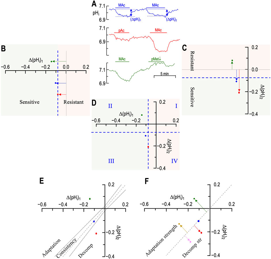
Figure 2. Plots of state, behavior, and behavior strength. (A) Three examples of experimental pH_i recordings. The blue record is from figure 3a of Bouyer et al. (2024); red, from figure 6a and green from figure 9a. (B) Graphical plot of “states” during the first challenge. The three horizontal arrows, with their tails on (ΔpH_i)₁ = 0, indicate the magnitude and direction of the pH_i change during challenge #1. According to the convention of Salameh et al., 2014, the vertical dashed blue line—again drawn at (ΔpH_i)/(ΔpH_o) = 40%—is the demarcation between the “resistant” and “sensitive” states. The green point in the positive territory indicates paradoxical alkalinization. (C) Graphical plot of “states” during the second challenge. The three vertical arrows, with their tails on (ΔpH_i)₂ = 0, indicate the magnitude and direction of the pH_i change during challenge #2. According to the convention of Salameh et al., 2014, the horizontal dashed blue line—drawn at (ΔpH_i)/(ΔpH_o) = 40%—is the demarcation between the “resistant” and “sensitive” states. (D) “State” diagram for twin challenges. This panel is an overlay of the previous two. I–IV indicate the quadrants formed by the two dashed blue lines. For example, the blue point in Q_III represents a neuron for which the state was sensitive for both challenges. (E) Hourglass plot for ‘behavior.’ The gray dashed line is the line of identity. For points lying on it (e.g., approximately true for blue point), (ΔpH_i)₂ = (ΔpH_i)₁. Points lying within the hourglass—formed by the upper and lower confidence limits defined by Salameh et al., 2014—define consistency of pH_i changes between the two challenges. Points above the hourglass represent adaptation; points below the hourglass represent decompensation (decomp). (F) Behavior strength (d_±, table 2 in Bouyer et al. (2024)). The arrows are orthogonal to the line of identity. Arrow length (units: pH) indicates adaptation strength (gold and green) or decompensation strength (pink and red points taken from figure 3 of Bouyer et al., 2024).

In Figure 2B, the single axis (i.e., x-axis) represents the (ΔpH_i)₁ for each of the three neurons in panel A. Following the “40%” definition of Salameh et al. (2014), the vertical dashed blue line represents the demarcation between “resistant” and “sensitive” neurons for (ΔpH_i)₁. Because ΔpH_o was 0.2, this blue line is 40% × 0.2 = 0.08 pH units to the left of where the y-axis would be (represented by the vertical gray line). The 40% figure emanates from a study of multiple cell lines and represents a natural break in the data (see Salameh et al., 2014). Because this figure is somewhat arbitrary, one could imagine adjusting it to match the degree of MAc or the nature of a disturbance (e.g., MAc vs. MAlk vs. RAc). We have chosen to adhere to the original definition to facilitate data comparisons.

• The red point representing (ΔpH_i)_1/pAc lies just to the left of the vertical dashed blue line because pAc₁ resulted in a pH_i decrease of 0.084 (i.e., the point is 0.084 to the left of the vertical gray line).

• The blue point lies slightly more to the left because (ΔpH_i)_1/MAc was −0.105.

• The green point lies further to the left because (ΔpH_i)_1/MAc was −0.141.

All three neurons are in the green (ΔpH_i)₁ sensitive zone.

In Figure 2C, the single axis (i.e., y-axis) represents (ΔpH_i)₂ for each of the same three neurons in panel A. The horizontal dashed blue line represents the demarcation between “resistant” and “sensitive” neurons for (ΔpH_i)₂ and is 0.08 pH units below where the x-axis would be (represented by the horizontal gray line).

• The red point representing (ΔpH_i)_2/MAc lies well below the horizontal dashed blue line because MAc₂ resulted in a pH_i decrease of 0.208 (the point is 0.208 below the horizontal gray line).

• The blue point lies only slightly below the blue line because (ΔpH_i)_2/MAc was −0.108.

• The green point lies paradoxically above the horizontal gray line because (ΔpH_i)_2/pMet↓ was +0.085.

The blue and red neurons are both in the green (ΔpH_i)₂ sensitive zone, whereas the green neuron is in the peach-colored (ΔpH_i)₂ resistant zone (which also includes paradoxical alkalinizations).

Figure 2D shows an overlay of panels B and C. The intersecting blue dashed lines now define four quadrants (Q):

• I. Any neurons in Q_I are resistant for both (ΔpH_i)₁ and (ΔpH_i)₂.

• II. Sensitive during (ΔpH_i)₁ → resistant during (ΔpH_i)₂.

• III. Sensitive during both (ΔpH_i)₁ and (ΔpH_i)₂

• IV. Resistant during (ΔpH_i)₁ → sensitive during (ΔpH_i)₂

Behavior

“Behavior” describes the change in ΔpH_i in the transition from the first to the second challenge. By definition, behavior has meaning only for two or more challenges. We term the graphical representation of behavior the “hourglass plot” (Figure 2E), which we build around the line of identity (LoI) that describes an experimental result, in which (ΔpH_i)₂ = (ΔpH_i)₁. This is the dashed gray line running from the lower left, through the origin, to the upper right. The curved parts of the hourglass represent confidence limits, as defined by Salameh et al. (2014) and described mathematically in equations 1 and 2 of the paper by Bouyer et al. (2024). Although the precise values of confidence limits are somewhat arbitrary, the hourglass provides an indication of the following behaviors:

• A “consistent” behavior is one in which the point representing the neuron lies within the hourglass, as typified by the blue neuron, which lies on the LoI.

• An “adaptive” behavior is one in which (ΔpH_i)₂ is sufficiently larger (in the algebraic sense) than (ΔpH_i)₁, that is, the point lies above the hourglass. The green neuron, although hardly typical, exhibits adaptation. A more typical example would fall between the x-axis and the upper bound of the hourglass.

• A “decompensating” behavior is one in which (ΔpH_i)₂ is sufficiently smaller (in the algebraic sense) than (ΔpH_i)₁, that is, the point lies below the hourglass, as typified by the red neuron.

Note that—as defined by Salameh et al. (2014)—a change in state does not necessarily produce an adaptive or decompensating behavior (the change in ΔpH_i must be sufficiently large). Conversely, the behavior can be adaptive or decompensating, although the state does not change (e.g., a point can be above or below the hourglass in Q_I).

Behavior strength

The hourglass analysis provides a useful visual display. However, from a quantitative perspective, it categorizes a cell only in a ternary fashion (i.e., adaptive, consistent, and decompensating) and can categorize a population only by referring to fractions of cells with particular behaviors. Bouyer et al. (2024) introduced two variations in these concepts, in which one computes the distance of a point to the LoI. Figure 2F shows five points. Blue, red, and green represent the three neurons from panel A; the pink and gold points are two arbitrary examples from figure 3b of the recent Bouyer paper. The dashed line associated with each point represents the distance from the point to the LoI.

In one variation, the distance is unsigned (d_Absolute)—all values are positive distances—so that average d_Absolute describes the dispersion of the points from the LoI.

In the other variation, the distance is signed d_±. Positive d_± values (e.g., gold and green points)—represent points above/to the left of the LoI and thus describe the strength of adaptation. Negative values (e.g., pink and red points) represent points below/to the right of the LoI and thus describe the strength of decompensation. The blue point lies virtually on the LoI and thus has a d_± value of ∼0. The mean d_± value of a population describes the overall direction and “behavior strength”—a term coined in the dissertation by Taki (2024). An advantage of the d_± approach is that one can perform statistical tests on populations of cells (e.g., wild-type vs. knockout).

Molecular basis of the effects of extracellular acid–base disturbances

We propose that the acute¹ response (e.g., state and behavior/d_±) of a cell to single or paired acid–base disturbances depends on a combination of three factors:

(1) near-instantaneous effects on the extracellular surface of acid–base transporters, both acid extruders (factor ‘1a’) and acid loaders (factor ‘1b’);

(2) extremely rapid effects on sensors (factor ‘2’) that detect changes in extracellular parameters and then rapidly modulate the transporters in factor ‘1’; and

(3) more slowly developing changes in cellular parameters that we will term “cellular constitution”—the collection of all ion-concentration, metabolic, and signaling properties that modulate factors ‘1’ and ‘2’ over the course of the challenge and that may persist to varying extents after the removal of the challenge. Note that the actions of factors ‘1’ and ‘2’ contribute to the constitution (factor ‘3’).

An important principle is that only factors ‘1’ and ‘2’ can influence pH_i over the first few seconds of a challenge. Later, gradually developing changes comprising ‘3’ can contribute not only to the pH_i time course during the challenge but also to the response to a subsequent challenge.

Before discussing factor ‘1’ through ‘3,’ we begin by considering the influences that cause pH_i to change or remain stable.

Fundamental law of pH_i regulation

Figure 3A illustrates the major acid-extrusion and acid-loading mechanisms in a cell such as a CNS neuron. Two reviews consider the detailed properties of these transporters, including sensitivity to acid–base challenges (Ruffin et al., 2025; Thornell et al., 2025).

Figure 3

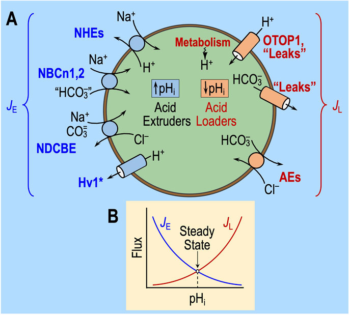
Figure 3. Regulation of intracellular pH. (A) Cell model of acid extruders (blue, on left) and acid loaders (red, on right). Acid extruders (some of which are shown in this figure) mediate the efflux of acid equivalents or the uptake of alkali equivalents. Acid loaders (some of which are shown in this figure, including cellular metabolism) mediate the uptake of acid equivalents or the efflux of alkali equivalents. Absent from this drawing are the electrogenic Na/HCO₃ cotransporters, which seem not to make a major contribution in neurons but are extremely important in astrocytes. Some, if not all, of the Na⁺-coupled “HCO₃⁻” transporters actually carry carbonate (CO₃⁼) or the NaCO₃⁻ ion pair. H⁺/monocarboxylate cotransporters are not present in this diagram. MCT1 in astrocytes mediates the efflux of lactate and H⁺ and thus operates as an acid extruder. The closely related MCT2 mediates the uptake of this lactate in neurons, where it behaves as an acid loader. *The voltage-gated proton channel Hv1 opens only at depolarized voltages and exhibits outward rectification (i.e., it operates as an acid extruder). (B) Kinetic model of pH_i regulation. The transmembrane flux is on the y-axis and pH_i on the x-axis. The shapes of the curves are for illustration only. J_E, rate of acid extrusion from all sources; J_L, rate of acid loading from all sources. When J_E = J_L, pH_i is stable. Surface/volume ratio and buffering power have no influence on steady-state pH_i. Cl/HCO₃ exchanger (AE); H_V1, voltage-gated H⁺ channel; Na-H exchangers (NHE); electroneutral Na-HCO₃ cotransporter (NBCn); Na-driven Cl/HCO₃ exchanger (NDCBE); other H⁺ channels (OTOP1).

As described previously (Roos and Boron, 1981; Boron, 2004; Bevensee and Boron, 2013; Occhipinti et al., 2020; Thornell et al., 2025), the fundamental law of pH_i regulation is

$\frac{d{\text{pH}}_{\mathrm{i}}}{d\mathrm{t}}=\frac{\rho }{\beta }\cdot \left(J_{\mathrm{E}}-J_{\mathrm{L}}\right).(10)$

Here, dpH_i/dt is the time rate of change of pH_i; ρ is the surface-to-volume ratio of the cell; β is total intracellular buffering power; J_E is the sum of the rates of all individual acid-extrusion processes (the rates of which are J_E1, J_E2, etc.), such as those on the left side of Figure 3A; and J_L is the sum of the rates of all individual acid-loading processes (the rates of which are J_L1, J_L2, etc.), such as those on the right side of Figure 3A.

As illustrated in Figure 3B, J_E tends to increase as pH_i decreases, whereas J_L tends to have the opposite pH_i dependence. In a steady state (i.e., when dpH_i/dt = 0), pH_i is stable because J_E = J_L. An acid–base challenge can initiate a change in pH_i (i.e., displace dpH_i/dt from 0) only by altering J_E and/or J_L, which, in turn, can occur only by producing near-instantaneous effects on transporters (factor ‘1,’ above) or sensors that rapidly regulate transporters (factor ‘2’). The subsequent time course of pH_i depends on evolving changes in J_E and J_L, which, in turn, must reflect changes in cellular properties—for example, ΔpH_i, Δ[HCO₃⁻]_i, Δ[CO₃⁼], and other downstream parameters—that secondarily modulate the pH_i dependence and other kinetic properties of transporters. Thus, the evolving pH_i dependencies of J_E and J_L determine the new steady-state pH_i, at which J_E and J_L come into balance during the challenge. These evolving changes could not only affect what we observe as the “state” during challenge #1, but they could also be sufficiently long-lasting to affect the “state” during challenge #2, thereby revealing themselves as “behavior.”

Note that changes in ρ or β cannot affect steady-state pH_i and, thus, cannot underlie a resistant/sensitive phenotype (i.e., state) or an adaptive/consistent/decompensative phenotype (i.e., behavior).⁵

Factor ‘1’: effects on acid–base transporters

In the following analyses, the effects of acid–base challenges on transporters would be rapid-onset/rapid-offset but, as noted in the previous section, could evolve during the challenge.

“Acidosis” (Ac)

In the absence of CO₂/HCO₃⁻, the only major acid–base transporters operative would be Na-H exchangers (NHEs) and H⁺ channels (Figure 4), as well as MCT2 monocarboxylate cotransporters, which mediate the cotransport of H⁺ and lactate. Although the physiological role of MCT2 is to import into neurons lactate generated by astrocytes (Ransom, 2017), the solutions in the paper by Bouyer et al. (2024) contain no lactate. Thus, to the extent that it operates, MCT2 would mediate H⁺/lactate efflux and—like the Na-H exchangers—function as an acid extruder. Independent of any allosteric effects, lowering pH_o would slow H⁺ efflux via both routes and thereby tend to lower pH_i, as indeed Bouyer et al. (2024) observed during Ac₁.

Figure 4

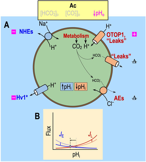
Figure 4. Effect of acidosis in the absence of CO₂/HCO₃⁻ (Ac) on transporters. (A) Cell model. In the nominal absence of extracellular CO₂/HCO₃⁻, “HCO₃⁻” transporters have a much-reduced effect on pH_i homeostasis. The metabolic production of CO₂, via the overall reaction CO₂ + H₂O → H⁺ + HCO₃⁻ (likely catalyzed by carbonic anhydrases), produces HCO₃⁻ but at levels that are most likely far lower than those observed under more physiological conditions. Thus, acid loading via HCO₃⁻ efflux is likely to be very low. The metabolically produced CO₂ itself exits the cell passively, either via the lipid phase of the membrane or channels (see Michenkova et al., 2021), and has no direct effect on pH_i. Not shown in this figure—the solutions used by Bouyer et al. (2024) did not contain lactate—is the H⁺/monocarboxylate cotransporter MCT2, which physiologically mediates lactate uptake into neurons and would likely be stimulated by acidosis. (B) Kinetic model. In this figure, with reduced “HCO₃⁻” transport even under control conditions, we show markedly reduced J_E (rate of acid loading from all sources) and J_L (rate of acid extrusion from all sources), as indicated by the semi-transparent blue and red curves. The more deeply colored curves indicate a J_E decrease and an J_L increase due to the effects of Ac on the pathways in panel (A). The horizontal arrow represents the anticipated effect on steady-state pH_i. Note that the removal of CO₂/HCO₃⁻ may lower, have no effect on, or increase steady-state pHi, depending on the initial pH_i and acid–base physiology of the cell. Boxes with “minus” symbols indicate inhibition, and magenta indicates a pH_o effect. Boxes with “plus” symbols indicate the corresponding stimulation. The struck-out Δ indicates no change. In the marquee, we indicate nominally absent parameters in gray. H_V1, voltage-gated H⁺ channel; J_E, acid-extrusion rate; J_L, acid-loading rate.

“Pure acidosis” or ↓pH_o (pAc)

In the presence of CO₂/HCO₃⁻ (Figures 5A, B), pAc would exhibit all the effects of Ac (↓ J_E and ↑ J_L), presumably tending to lower pH_i. In addition, pAc would lead to a modest decrease in [CO₃⁼]_o, which (because the Na⁺-coupled HCO₃⁻ transporters appear to carry a form of CO₃⁼; see Lee et al., 2023) would lead to a further (with respect to the one that we predict in Ac), albeit modest, decrease in J_E and, thus, a decrease in pH_i. Finally, it is possible that the decrease in pH_o would have allosteric effects on various acid–base transporters, although we cannot infer the net direction without resorting to a more sophisticated quantitative approach (see Discussion).

Figure 5

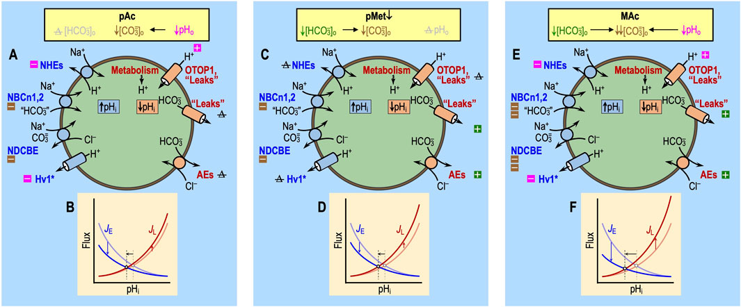
Figure 5. Effect of pAc, pMet↓, and MAc on transporters. Note that the only factors that can contribute to the initial (i.e., near-instantaneous) dpH_i/dt induced by an extracellular challenge are those that immediately impact proteins facing the extracellular fluid: (1) acid–base transport pathways (including “leaks”), like those in the incomplete list shown here, and (2) rapidly responding extracellular sensors, like those shown in Figure 6. Later during the challenge, other pathways can come into play as cellular constitution changes and indirectly impacts acid–base transporters. (A) Pure acidosis: cellular model. The decrease in pH_o per se (magenta symbols) will produce the direct inhibition of Na-H exchangers (NHEs) and the voltage-gated H⁺ channel Hv1 and direct stimulation of other H⁺ channels like OTOP1 and “leakage” (i.e., unidentified) pathways. Indirectly, the decreased pH_o will lower [CO₃⁼]_o (brown symbols), which will slow Na⁺-driven HCO₃⁻ transporters—the Na⁺-driven Cl-HCO₃ exchanger NDCBE and the electroneutral Na/HCO₃ cotransporters NBCn1 and NBCn2—that are known or believed to carry some form of CO₃⁼. We expect true HCO₃⁻ pathways to be unaffected by pAc because [HCO₃⁻]_o per se does not change. Note: pAc indicates an isolated pH_o decrease in the presence of CO₂ and HCO₃⁻ not to be confused with Ac in Figure 4, which indicates an isolated pH_o decrease in the absence of CO₂ and HCO₃⁻. (B) Pure acidosis: kinetic model. The semi-transparent curves—blue for J_E (rate of acid loading from all sources) and red for J_L (rate of acid extrusion from all sources)—represent control conditions and are the same as in Figure 3B. The more deeply colored curves indicate a J_E decrease and a J_L increase, both are consequences of the effects of pAc on the pathways in panel (A). The horizontal black arrow represents the anticipated effect on steady-state pH_i. (C) Pure metabolic/down: cell model. The decrease in [HCO₃⁻]_o per se (green symbols) is expected to produce the direct stimulation of HCO₃⁻ leakage pathways and Cl-HCO₃ exchange via anion exchangers (AEs) and indirect inhibition of Na⁺-coupled HCO₃⁻ transporters, slowing down Na⁺-driven HCO₃⁻ transporters, which either are known or believed to carry some form of CO₃⁼. We expect true H⁺ pathways to be unaffected by pMet↓ because pH_o per se does not change. (D) Pure metabolic/down: kinetic model. The meanings of the curves and symbols are the same as in panel B, compared to which we expect smaller effects on J_E but larger effects on JL. The horizontal arrow indicates that the decrease in pH_i is approximately the same length as in panel (B). The data from Bouyer et al. (2024) indicate that this panel-D arrow should only be ∼40% as long as that in panel (B). We propose that the difference could be due to the stimulatory effect of an extracellular HCO₃⁻ sensor (see Figure 6) that would increase J_E under the conditions of pMet↓. (E) Metabolic acidosis: cell model. Here, we superimpose the effects of panels A and C. (F) Metabolic acidosis: kinetic model. Here, we superimpose the effects of panels B and D, generating a larger decrease in steady-state pH_i than each alone. The result of simply adding ΔpH_i effects in panels B and D is greater in magnitude than ΔpH_i actually observed by Bouyer et al. (2024). The reason, as suggested in the legend for panel D, may be that extracellular HCO₃⁻ sensors (see Figure 6) reduce the decrease in pH_i caused by pMet↓ (see Figure 10). Boxes with “minus” symbols indicate inhibition; green indicates an effect of [HCO₃⁻]_o per se; magenta indicates a pH_o effect; and brown indicates a [CO₃⁼]_o effect. Boxes with “plus” symbols indicate the corresponding stimulation. The struck-out Δ value indicates no change. In the marquee, we indicate the unchanged parameters in gray. J_E, acid-extrusion rate; J_L, acid-loading rate.

“Pure metabolic” or ↓[HCO₃⁻]_o (pMet↓)

Still considering events occurring in the presence of CO₂/HCO₃⁻, pMet↓ (Figures 5C, D) would have only one of the predicted effects of pAc: with pMet↓, the decrease in [HCO₃⁻]_o would lower [CO₃⁼]_o and thus modestly reduce J_E. The decrease in [HCO₃⁻]_o would also accelerate the efflux of HCO₃⁻ via the Cl-HCO₃ exchanger AE3, thereby increasing J_L. Thus, the effects of pMet↓ on both J_L and J_E would tend to lower pH_i.

Metabolic acidosis (MAc)

Finally, the impact of MAc (Figures 5E, F) strictly on acid–base transporters ought to be approximately the sum of the individual impacts of pAc and pMet↓, adjusted for the non-additive effects on [CO₃⁼]_o, as discussed by Bouyer et al. (2024).⁶

In this section, we have limited ourselves to the direct effects of challenges on acid–base transporters. In the next two sections, we will see that these are only the first part of the story: ΔpH_o and Δ[HCO₃⁻]_o also have direct effects on sensors and indirect effects on cellular constitution, both of which are likely to modulate acid–base transporters and thus affect the pH_i time course. Later, we will consider the combined effects of acid–base disturbances on all three factors, namely, transporters, sensors, and constitution.⁷ Moreover, Figure 11 illustrates the apparent additivity of pAc₁ and pMet↓₁. In conjunction with Figure 13, we will discuss the non-additivity of pAc₂ and pMet↓₂.

Factor ‘2’: effects on sensors of the extracellular acid–base status

The introduction of the paper by Bouyer et al. (2025), the review by Ruffin et al. (2025), and the work by Thornell et al. (2025) summarize several classes of acid–base sensors. GPR68 (OGR1) is one of at least four pH_o-sensitive G-protein-coupled receptors (GPCRs) and is present in medulloblastoma tissue (Huang et al., 2008), rat HC neurons (Schneider et al., 2012), and rat anterior pituitary gland (Horiguchi et al., 2014). Figure 6 depicts GPR68, in particular, and the presumed effects of MAc. HC acid-sensing ion channels (ASICs) (Alvarez et al., 2003) could play a role as pH_o-sensors. On the other hand, although the tandem pore domain acid-sensing K⁺ (TASK) channels are present in multiple brain regions (Lesage, 2003), they are not in the hippocampus. Finally, the putative extracellular CO₂/HCO₃⁻ sensors, RPTPγ and RPTPζ, are widely distributed in the CNS (Müller et al., 2004; Hayashi et al., 2005; Lamprianou et al., 2006) and could potentially contribute to the pH_i physiology in the study by Bouyer et al. (2024). Recent work by Taki et al. (2024) shows that murine HC neurons (but not astrocytes) express both RPTPγ and RPTPζ. Moreover, in her PhD dissertation, Taki (2024) showed that the global knockout of RPTPζ in mice greatly reduces the ability of HC neurons to resist the pH_i decrease caused by MAc or RAc.

Figure 6

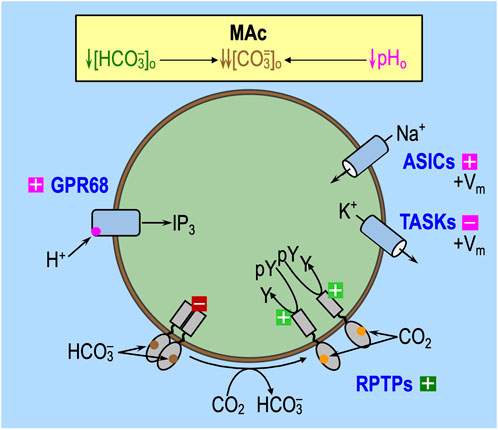
Figure 6. Effect of MAc on extracellular acid–base sensors. Note that the only factors that can contribute to the initial (i.e., near-instantaneous) dpH_i/dt induced by an extracellular challenge are those that immediately impact proteins facing the extracellular fluid: (1) acid–base transport pathways (including “leaks”), like the ones in the incomplete list shown in Figure 5E, and (2) rapidly responding extracellular sensors, like the ones shown here. Later during the challenge, other pathways can come into play as cellular constitution changes and indirectly impacts acid–base transporters. GPR68 (OGR1) and at least three other G-protein-coupled receptors can sense H⁺ or a pH_o⁻ sensitive metabolite and lead to an increase in IP₃/Ca²⁺. The ASICs and TASKs are families of pH_o⁻ sensitive channels. In both cases, decreases in pH_o lead to depolarization of the membrane, which, in turn, could have other signaling effects. In cells (e.g., astrocytes) with substantial electrogenic Na/HCO₃ cotransporter activity, MAc would lead to decreased Na⁺ and CO₃⁼ influx (or increased efflux), with the effect of augmenting depolarization. RPTPγ and RPTPζ have, in common, the presence of an extracellular carbonic-anhydrase–like domain (CALD), hypothesized to bind either HCO₃⁻ or CO₂. In the monomeric state—hypothesized to be favored by low [HCO₃⁻]_o—the active tyrosine phosphatase dephosphorylates tyrosine residues. Extracellular boxes with “minus” symbols indicate inhibition, and magenta indicates an effect of low pH_o per se. Extracellular boxes with “plus” symbols indicate stimulation by low pH_o (magenta) or low [HCO₃⁻]_o (dark green). The intracellular dark-red box with a “minus” symbol indicates blockade of tyrosine phosphatase activity. The light-green box with a “plus” symbol indicates an active tyrosine phosphatase. IP₃, inositol trisphosphate; pY, phosphotyrosine group; Y, tyrosine.

The activation of extracellular acid–base sensors, with a slight delay, could modulate the activity of acid–base transporters and thereby contribute to—or oppose—the initiation of pH_i changes predicted in Figure 5 during an acid–base challenge. The continuing actions of these extracellular sensors—that is, their effects on transporters and cellular constitution—likely impact the evolution of the pH_i change later during the challenge and produce longer lasting effects that influence “behavior” in the second of two challenges.

Effect of pAc on extracellular sensors

In the experiments of Bouyer et al. (2024), Ac (see Figure 4) and pAc (see Figures 5A, B) could act through pH-sensitive GPCRs and ion channels, which, in principle, could alter the (J_E–J_L) balance and thereby contribute to “state” (i.e., resistance vs. sensitivity). In Figure 6, the magenta “plus” and “minus” symbols indicate the anticipated effects of pAc on extracellular sensors.

Effect of pMet↓ on extracellular sensors

With pMet↓ (see Figures 5C, D), the decreased [HCO₃⁻]_o would trigger HCO₃⁻ sensors (Figure 6). In the experiments of Bouyer et al. (2024), pMet↓₁ is unique among acid–base challenges in producing only about half the acidification of the other challenges (i.e., MAc₁, Ac₁, and pAc₁). pMet↓ could promote monomerization of RPTPγ (see Figure 6), as suggested by preliminary data (Moss et al., 2018), and thereby increase the tyrosine phosphatase activity. In renal proximal tubules, it appears that this action would increase J_E. Following this logic, pMet↓—acting through RPTPγ (and possibly also RPTPζ)—could promote a resistant state and, if persistent, could promote adaptation behavior in a later challenge. In Figure 6, the dark-green extracellular “plus” symbol indicates the anticipated effects of pAc on extracellular sensors.

Effect of MAc on extracellular sensors

The most straightforward hypothesis might be that the integrated “sensor” effects of pAc and MAc, described above (Figure 6), would summate to produce the integrated “sensor” effects of MAc (see extracellular “plus” and minus symbols in Figure 6). This may or may not be true in naïve neurons, as shown in Figure 8. However, for neurons previously exposed to MAc₁, the integrated “sensor” effects of pAc₂ and pMet↓₂ may interfere with one another, as hypothesized in the discussion of Figure 14.

Factor ‘3’: effects on cellular constitution

The effects of acid–base disturbances on transporters (see factor ‘1,’ just above) and extracellular sensors (see factor ‘2,’ above) could begin instantaneously or nearly so and continue throughout the challenge (Figure 7). Although, upon the removal of the challenge, the effects on transporters and sensors per se may cease just as instantaneously as they had commenced, the more slowly developing consequences of altered transporter activity on intracellular solute concentrations (e.g., pH_i, [HCO₃⁻]_i, [CO₃⁼]_i, [Na⁺]_i, and [Cl⁻]_i), membrane potential (V_m), and of altered sensor activation on downstream signaling pathways (e.g., phosphorylation state and protein trafficking) could evolve during the acid–base challenge and also persist for some time.⁸ In addition to constitutional changes produced directly by acid–base transporters (‘1’) and extracellular sensors (‘2’), indirect influences could include myriad effects. For example, V_m changes could affect voltage-sensitive channels and transporters and thereby affect neuronal firing and such parameters as [Ca²⁺]_i. Alterations in ion concentrations would impact transporters and channels other than those depicted in Figure 3. For example, increased [Na⁺]_i would stimulate the Na–K pump, which would tend to lower [Na⁺]_i, increase [K⁺]_i, and hyperpolarize the cell. Changes in pH_i could directly impact pH_i sensors (reviewed by Thornell et al., 2025) and—because [HCO₃⁻]_i changes in the same direction as pH_i—could secondarily impact the soluble adenylyl cyclase sAC (Chen et al., 2000), present in some HC axon terminals (Chen et al., 2013). In locus coeruleus chemosensitive neurons, the activation of sAC increases L-type Ca²⁺-currents and limits the hypercapnia-induced increase in the firing rate (Imber et al., 2014).

Figure 7

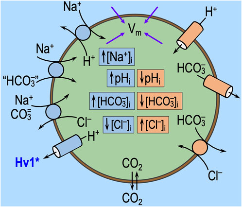
Figure 7. Direct effects of acid–base transport on V_m and intracellular ion concentrations. In this figure, we show the acid–base transport pathways from Figure 3, with blue and peach-colored boxes indicating the normal effects of these pathways on intracellular pH (pH_i) and ion concentrations. We also show membrane potential (V_m), which is determined by intracellular solute concentrations and the state of ion channels and electrogenic transporters. Extracellular acid–base disturbances, like those shown in Figure 5, trigger direct changes in transport activity. Extracellular acid–base sensors (see Figure 6) may modulate this transporter activity. If these transport pathways undergo net stimulation (or inhibition), the concentration changes shown in this figure will be accentuated (or attenuated). The arrows leading to V_m indicate that the rapid extracellular challenges or slower intracellular concentration changes can alter V_m. In addition to the “direct” effect of changes in transport on the cellular constitution and the “secondary” effects of the extracellular sensors, we expect more complex changes to evolve over time. These complex changes could affect a myriad of membrane proteins and metabolic/signaling pathways, thereby altering the activity of the acid–base transport pathways in ways that influence “state” and “behavior.”

The above mentioned effects could produce changes in the number of acid–base transporter proteins in the plasma membrane (due to trafficking, protein degradation, and eventually protein synthesis) and changes in their unitary or “per-molecule” activities (due to alterations in intracellular ionic and post-translational modifications). Thus, the “functional activity” of transporters (i.e., protein number × unitary activity) underlying many J_E1, J_E2, … and J_L1, J_L2, … terms introduced in our introduction of Equation 10 may change over the evolution of the acid–base disturbance and then persist for some time.

Taki (2024) suggests that in a MAc–MAc protocol, progressively lower and lower pre-MAc₂ pH_i values correlate with an increase in the degree of adaptation behavior. Because higher pH_i values just before MAc₂ translate to higher [HCO⁻₃]_i values just before MAc₂ (assuming that CO₂ has equilibrated across the cell membrane), it is possible that sAC (which senses cytoplasmic HCO₃⁻) could participate in neuronal state and/or behavior. Other pH_i-sensitive processes could respond during a challenge, and the extracellular sensors could affect these or vice versa.

In acutely dissociated HC CA1 neurons, Brett et al. (2002) have shown that the inhibition of protein kinase A (PKA) inhibits Cl-HCO₃ exchange but stimulates Na⁺-dependent Cl-HCO₃ exchange, thereby increasing pH_i in low-pH_i neurons. In high-pH_i neurons, the effects are the opposite. The stimulation of PKA has the opposite set of effects. In the protocols of Bouyer et al. (2024), decreases in pH_o could have activated pH_o⁻ sensitive GPCRs that elevate [cAMP]_i (Radu et al., 2005) and thereby contributed to state and behavior.

Determinants of neuronal state and behavior

Even before the work of Bouyer et al. (2024), Bouyer et al. (2004) had shown that some HC and medullary raphé neurons exhibit smaller pH_i decreases than other neurons—what Salameh et al. (2014) would later term MAc resistance vs. sensitivity. Salameh et al. (2014) later showed that resistance/sensitivity and adaptation, consistency and decompensation phenotypes occur in multiple cell types other than HC neurons and astrocytes.

We hypothesize that state—resistance vs. sensitivity—depends both on the pre-existing status of the three factors discussed above and how constitutional changes evolve during the challenge. The pre-existing status, which could reflect the previous history of acid–base and other challenges, comprises the kinetic properties of each acid–base transporter and all factors (e.g., the impact of extra- and intracellular sensors) that influence these kinetic parameters.

We hypothesize that behavior—adaptation vs. consistency vs. decompensation—depends on all of the elements that determine the state during the first of two challenges and the persistence of all changes in cellular parameters from the first challenge to the next. Presumably, these parameter changes eventually extinguish with time. However, to the extent that the changes persist, they represent a sort of memory of the previous challenge that influences how a cell responds to a future challenge. Examples of persistent changes could include alterations in the numbers of various acid–base transporters and sensors that are resident in the plasma membrane, their post-translational states, and cellular constitution.

Although it was outside the scope of the study by Bouyer et al. (2024), it would be illuminating to examine the challenges opposite to those in that study (i.e., metabolic alkalosis or MAlk, pure alkalosis or pAlk, and pure metabolic/upward or pMet↑), as well as respiratory acidosis (RAc) and alkalosis (RAlk), pure respiratory/up (an isolated increase in [CO₂]_o or pR↑), and pure respiratory/down (pR↓). Note, however, that in the study by Bouyer et al. (2004), it was MAc—not RAc, MAlk, or RAlk—that seemed to generate pH_i responses that were the most idiosyncratic.

State: resistance vs. sensitivity

Salameh et al. (2014) defined MAc-resistant cells as those for which pH_i decreases by <40% of ΔpH_o. Regardless of where one draws the dashed blue lines in Figures 2B, D, some cells will be more resistant/sensitive than others. Bouyer et al. (2024) observed a continuum of ΔpH_i values that presumably depend on the factors noted in the previous section:⁹ rapid effects on ‘1’ acid–base transporters, ‘2’ extracellular acid–base sensors, and ‘3’ more slowly developing effects on cellular constitution. Figure 8A summarizes the interdependence of factors ‘1’–‘3’ for a naïve cell with an “average¹⁰” pH_i decrease during MAc₁. The initial (i) steady-state pH_i (i.e., pH_i prevailing just before MAc) is described by the intersections of the semi-transparent blue and red curves. We now discuss the impact of MAc₁ on cells in four different states—sensitive and resistant plus “average” and “paradoxical” (an extreme variant of resistant)—and then raise the issue of how pAc₁ and pMet↓₁ contribute to MAc₁.

Figure 8

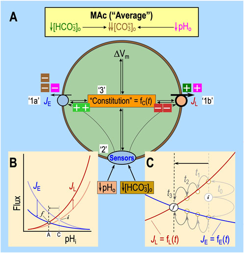
Figure 8. Model of average “state” during MAc. (A) Cellular model of the effects of MAc. In this figure, we suppose a state response to MAc that is on the border of resistant and sensitive—that is, “average.” The blue J_E symbol represents the total flux mediated by all mechanisms of acid extrusion (factor ‘1a’), whereas the red J_L symbol includes fluxes of all mechanisms of acid loading (factor ‘1b’ in white box). The oval “Sensors” symbol includes all sensors that respond to changes in [HCO₃⁻]_o or pH_o (factor ‘2’). RPTPγ and RPTPζ presumably also respond to changes in [CO₂]_o, which did not occur in the experiments conducted by Bouyer et al. (2024). The extracellular dark-green, brown, and magenta “plus” and “minus” symbols have the same meaning as detailed in the previous figures (i.e., indicating which aspect of the MAc challenge produces the stimulation or inhibition, as shown in Figure 5E). The intracellular light-green “plus” and dark-red “minus” symbols (emanating from “Sensors” and Constitution) indicate enhancement or depression. Although we show equal numbers of intracellular light-green “plus” symbols and red “minus” symbols, it is really some combination of the two that reflects the relative degrees of transporter stimulation/inhibition by “Sensors” and/or “Constitution.” The black double arrows indicate that J_E influences cellular constitution (factor ‘3’) and vice versa. The same holds true for ΔV_m, J_L, and the hypothesized sensors (see Figure 6) for extracellular H⁺ (e.g., GPR68) and HCO₃⁻ (e.g., RPTPγ and ζ). Note that we hypothesize that constitution is a function of time. (B) Kinetic model. This panel is a reproduction of the material shown in Figure 5F. (C) Higher magnification view of the kinetic model shown in panel (B). As illustrated in panel B, MAc instantly causes the J_E curve to shift downward and the J_L curve to shift upward, as indicated by the more deeply colored blue and red curves, respectively. In this figure, in panel C, we reproduce, at higher magnification, the newly shifted J_E (blue) and J_L (red) curves, the two vertical dashed lines, the horizontal arrow, and the points that we label “i” (initial) and “f” (final). Before MAc, the semi-transparent blue and red curves (shown in panel B but not C) passed through point “i.” Upon the imposition of MAc, at time “t₀,” the J_E value instantaneously jumps upward to meet the more deeply colored red curve, as indicated by the upper light gray arrow, and the J_L value instantly jumps downward to meet the more deeply colored blue curve. Because J_L > J_E, that is, Δ(JE–JL) is negative, pH_i begins to decrease at its maximal rate for this experiment. As pH_i decreases (moving leftward on red and blue curves), J_L decreases and J_E increases. After time t₁, Δ(JE–JL) is still negative but to lesser extent than at time t₀. Thus, pH_i decreases more slowly, eventually reaching time t₃, where J_E and J_L come back into balance—that is, Δ(JE–JL) = 0—so that pH_i is in a new, lower steady state at point “f” than during control conditions at point “i.” Because cellular constitution changes during the MAc challenge, J_E and J_L are both functions of time.

“Average” cells

Viewed in the context of Equation 10, for all but a small fraction of cells with paradoxical responses (discussed below¹¹), the imposition of MAc temporarily shifts the difference (J_E–J_L) in the negative direction (see Figure 8B), initiating a decrease in pH_i that plays out over several minutes. At the instant of the switch to MAc (see Figure 8C, t₀), pH_i has not yet changed. Nevertheless, J_E jumps to the new J_E vs. pH_i curve (bright blue), which we presume to be below the original one. Simultaneously, J_L jumps to the new J_L vs. pH_i curve, which we presume to be above the original one.¹² As a result, J_L exceeds J_E at t₀, and pH_i begins to decrease at a rate determined by ρ, β, and Δ(J_E–J_L) in Equation 10. As pH_i declines, J_E increases gradually (t₁, t₂, and t₃) and J_L decreases. At t₃, J_E and J_L have once more attained a balance at the final (f) steady state. Although Figure 8C depicts the J_E and J_L curves as being static (i.e., having fixed shapes and positions in the two-dimensional space of the chart), the shapes and positions of J_E vs. pH_i and J_L vs. pH_i could evolve over time, in response to changes in the extracellular sensors and cellular constitution, both of which potentially impact J_E and J_L.

Sensitive cells

For cells that respond to MAc with a relatively large pH_i decrease, the net effect of MAc on factors ‘1’–‘3’ must be to produce a highly negative Δ(J_E–J_L) over the period of the MAc challenge. Some neurons are unusually sensitive to MAc. For example, examination of figures 3b, 5b, 7b, and 9b in Bouyer et al. (2024) reveals that, during MAc₁, some HC neurons (a total of 35 out of 230 or ∼15.2%) exhibit a decrease in pH_i that is even greater in magnitude than the decrease in pH_o during MAc; in other words, (ΔpH_i)_1/MAc < −0.20. In these neurons, MAc₁ must have produced a sufficiently large negative shift in Δ(J_E–J_L), integrated over the period of the challenge, to produce an unusually large intracellular acidification. In the cell model of Figure 9A, we imagine that MAc causes a large decrease in J_E and a large increase in J_L. In Figure 9B, we imagine a large downward shift (or a shallower slope) in the J_E curve and a large upward shift (or steeper slope) in the J_L relationship. Either a sufficiently large J_E downshift or J_L upshift could produce a highly negative Δ(J_E–J_L) and thus a highly MAc-sensitive state.

Figure 9

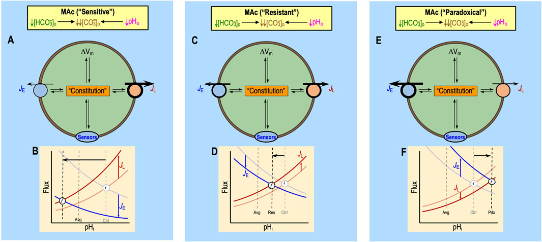
Figure 9. Models of sensitive, resistant, and paradoxical states during MAc. We hypothesize that MAc produces the usual initial percent inhibition (extracellular “minus” symbols) or stimulation (extracellular “plus” symbols) of each transporter (see Figure 5E) and sensor (see Figure 6), regardless of the subsequent pH_i response that is indicative of state—sensitive, resistant, or paradoxical (exaggerated version of resistant). Instead, differences in the state would reflect differences in (1) transporter numbers, (2) sensor numbers, and (3) cellular constitution (which would influence the intrinsic transporter and sensor activity). In the cellular model panels (A, C, E), the thicknesses of arrows for J_E (rate of acid loading from all sources) and J_L (rate of acid extrusion from all sources) reflect functional activities (i.e., product of the protein number and intrinsic activity per protein). In the kinetic model panels (B, D, F), the semi-transparent curves (blue for J_E and red for J_L) are the same as the curves shown in Figure 3B; their intersections reflect initial (i) pH_i values. The more deeply colored curves indicate the hypothetical J_E and J_L curves that prevail in each of the three states, and their intersections reflect final (F) pH_i values. The horizontal black arrows represent the anticipated effect on steady-state pH_i (i.e., i → (F). (A) MAc-sensitive neuron: cellular model. The sensitive state, reflecting the status of sensors and cellular constitution, results in some combination of depressed acid extrusion and elevated acid loading. (B) MAc-sensitive neuron: kinetic model. The deeply colored curves indicate a large J_E decrease and a large J_L increase due to the effects of MAc on the pathways in panel A for this neuron with a sensitive state. The result is a large decrease in steady-state pH_i. Note: these two curves are the most exaggerated J_E and J_L curves, compared to the “average” cell shown in Figure 8, “resistant” cell shown in Figure 9C, and “paradoxical” cell shown in Figure 9E. (C) MAc-resistant neuron: cellular model. The resistant state, reflecting the status of sensors and cellular constitution, results in some combination of a modest J_E decrease and a modest J_L decrease, both of which are in opposite directions compared to the “sensitive” neuron shown in Figure 9A, “average” shown in Figure 8, and “paradoxical” shown in Figure 9E. (D) MAc-resistant neuron: kinetic model. The deeply colored curves indicate only a modest J_E decrease vs. the larger one in panel (B) and a modest J_L increase vs. the larger one in panel (B) due to the effects of MAc on the pathways in panel C for this neuron with a resistant state. The result is only a modest decrease in steady-state pH_i. (E) paradoxical response to MAc: cellular model. The paradoxical response is an extreme variant of the resistant state and reflects that the status of sensors and cellular constitution results in some combination of a robust increase in J_E and a modest decrease in J_L. Note that the directions of these changes are opposite those of the “sensitive” neuron shown in Figure 9A, the “average” neuron shown in Figure 8, and the “resistant” neuron shown in Figure 9C. We propose a possible cellular mechanism of the paradoxical responses to MAc₁ shown in Figure 10. (F) Paradoxical response to MAc: kinetic model. The deeply colored curves indicate some combination of a robust J_E increase (vs. the decreases in the other examples) and a modest J_L decrease (vs. the increases in the other panels) due to the effects of MAc on the pathways in panel E for this paradoxical neuron. The result is an increase in steady-state pH_i.

Resistant cells

For cells that respond to MAc with a relatively small pH_i decrease, the net effect of MAc on factors ‘1’–‘3’ must be to produce a negative Δ(J_E–J_L) that is relatively small in magnitude. In the cell model of Figure 9C, we assume that MAc causes a modest decrease in J_E and a modest increase in J_L. Figure 9D represents these J_E/J_L changes as a more modest J_E downshift and J_L upshift, although either effect could dominate to produce a modestly negative Δ(J_E–J_L) and thus a highly MAc-resistant state.

Salameh et al. (2017) revealed an interesting mechanism by which HC neurons mitigate the decrease in pH_i during MAc, a process that depends on changes in cellular composition. In HC neurons cultured from WT mice, MAc tends to induce a pH_i decrease that is initially rapid but limited in magnitude (Salameh et al., 2017). However, in HC neurons cultured from mice genetically deficient in the Cl-HCO₃ exchanger AE3 (an acid loader), MAc induces a relatively slow initial decrease in pH_i (reflecting the absence of AE3 and thus a smaller, initial MAc-induced negative shift in J_L) that continues for some time. The result is a slow but large decrease in pH_i. Salameh et al argued that, in WT neurons, the robust activity of AE3 loads the cell with Cl⁻, which, in turn, increases J_E by stimulating both the Na⁺-driven Cl-HCO₃ exchanger and NHEs, which often have a positive dependence on [Cl⁻]_i (see Parker, 1983; Davis et al., 1994; Rajendran et al., 1995, 1999; Hogan et al., 1997; Bevensee et al., 1999). We interpret this hypothesized increase in [Cl⁻]_i as a gradual change in cellular constitution that progressively increases J_E over time and thereby tends to bring J_E and J_L into balance at a relatively high pH_i—that is, the WT neurons appear to be relatively resistant to MAc. Thus, we would expect that neurons with relatively high functional activities of AE3, NDCBE, or NHE would tend to be more MAc-resistant, whereas neurons with lower functional activities would tend to be more MAc-sensitive.

Paradoxical responses

Returning to the paper by Bouyer et al. (2024), an examination of their figures 3b, 5b, 7b, and 9b—all of which have MAc as challenge #1—reveals that, during MAc₁, a small fraction of HC neurons (a total of 22 out of 230 or ∼9.6%) exhibit a paradoxical alkalinization. In other words, for these 22 neurons, (ΔpH_i)_1/MAc > 0, so the points representing each lie to the right of the y-axis in a state diagram like that in Figure 2D. The net effect of MAc₁ in these 22 paradoxical neurons must have been to produce an immediate and sustained positive shift in Δ(J_E–J_L), as illustrated in Figures 9E, F.

Analogous to the 22 paradoxical pH_i increases discussed above is a non-physiological case that results from exposing naïve neurons to pMet↓. As summarized in figure 8b of Bouyer et al. (2024), 20 of 52 neurons (38%) alkalinized in response to pMet↓₁.

We are unaware of any mechanism through which MAc₁ (see Figures 5E, F) or pMet↓₁ (see Figures 5C, D) could act directly on transporters to produce such an immediately positive, paradoxical pH_i increase. Rather, it is more likely that, in a subset of neurons, extracellular sensors detect the decrease in [HCO₃⁻]_o (in MAc₁ or pMet↓₁) and/or pH_o (in MAc₁) and respond by producing a marked and extremely rapid increase in (J_E–J_L) that overwhelms the more typical acidifying effects of MAc₁ (Figures 8, 9A–F) and pMet↓₁.

Given that (1) an isolated decrease in basolateral [HCO₃⁻]_o (delivered via an OOE solution) acutely increases J_E in renal PTs (Zhou et al., 2005), (2) PTs are insensitive to acute, isolated decreases in basolateral pH_o (OOE solution) during this time frame (Zhou et al., 2005), (3) the PT response requires RPTPγ (Zhou et al., 2016), and (4) RPTPγ and RPTPζ are present in virtually every mouse HC neuron (Taki et al., 2024), we propose the following mechanism (Figure 10) by which the ∼10% of naïve HC neurons subjected to MAc₁ and the nearly 40% subjected to pMet↓ exhibit a paradoxical pH_i increase: the decrease in [HCO₃⁻]_o triggers the monomerization of RPTPγ or RPTPζ (see Figure 6), leading to the dephosphorylation of certain phosphotyrosines and, as a consequence, the rapid stimulation of acid extruders and/or inhibition of acid loaders.

Figure 10

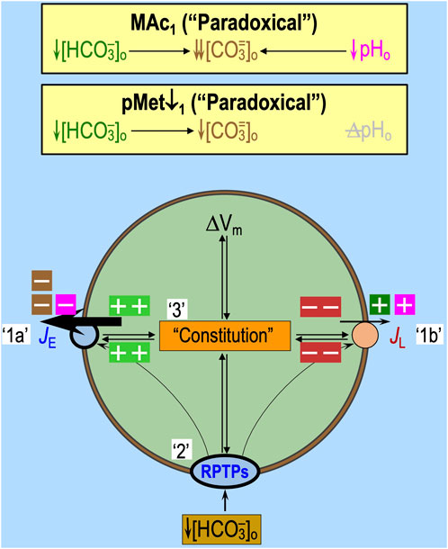
Figure 10. Hypothesized mechanistic model, for a naïve HC neuron, of paradoxical pH_i increases induced by MAc or pMet↓. We hypothesize that MAc₁ produces the usual initial percent inhibition (extracellular brown or magenta “minus” symbols) or stimulation (extracellular dark-green or magenta “plus” symbols) of each transporter (see Figure 5E) and sensor (see Figure 6), regardless of the subsequent pH_i response indicative of state. pMet↓₁ would produce only the effects indicated by extracellular dark-green and brown “minus” and “plus” symbols (i.e., not magenta symbols). Compared to other naïve neurons, the paradoxical responses to MAc₁ or pMet↓₁ (state) would reflect differences in (1) transporter numbers, (2) sensor numbers, and (3) cellular constitution (which would influence intrinsic transporter and sensor activity). The thicknesses of the arrows for J_E (rate of acid loading from all sources) and J_L (rate of acid extrusion from all sources) and the RPTPs (oval) reflect functional activities (i.e., product of the protein number and intrinsic activity per protein). The intracellular light-green “plus” symbols and red “minus” symbols indicate the relative effects of cellular constitution (including signaling from RPTPs) on J_E and J_L. Although we show equal numbers of intracellular light-green “plus” symbols and red “minus” symbols, it is really some combination of the two that reflects the relative degrees of transporter stimulation/inhibition by “Sensors” and/or “Constitution.” We predict that pMet↓₁, lacking the pH_o effects of MAc₁, would have relatively more light-green “plus” symbols and fewer red “minus” symbols, thus indicating a greater net increase in Δ(J_E–J_L) and a greater paradoxical pH_i increase than MAc₁.

Additivity of pAc₁ and pMet↓₁

The data from Bouyer et al. (2024) show that, in naïve neurons, the average ΔpH_i elicited by pAc₁ and the average ΔpH_i elicited by pMet↓₁ approximately summate to the average ΔpH_i elicited by MAc₁ in a population of rat HC neurons. The reported contributions were ∼70% for pAc₁ and ∼30% for pMet↓. Figure 11 illustrates how this additivity could occur in a single “average” neuron. Considering only the direct effects of acid–base disturbances on transporters—that is, without the effect of the hypothesized extracellular H⁺ and HCO₃⁻ sensors—we predicted that the ΔpH_i effect of pMet↓₁ would have been similar to that of pAc₁, so the two would have summed to a ΔpH_i value greater than that produced by MAc₁. Thus, we hypothesize that in naïve HC neurons, the effect of decreased pH_o on extracellular-H⁺ sensors produces a relatively weak stimulation of acid extrusion overloading (i.e., weak opposition to the pH_i decrease), whereas the effect of decreased [HCO₃⁻]_o produces a relatively strong stimulation (i.e., strong opposition to the pH_i decrease).

Figure 11

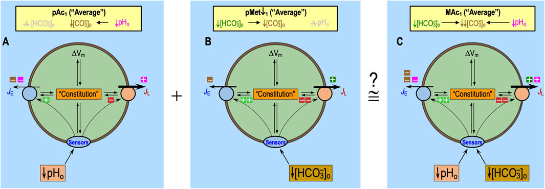
Figure 11. Hypothesized cellular mechanism, for naïve neurons, of additivity: pAc₁ + pMet↓₁ ≅ MAc₁. (A) Effect of pure acidosis on an “average” HC neuron. We hypothesize that the decrease in pH_o stimulates only one class of sensors (e.g., GPR68) with relatively weak functional activity. (B) Effect of pure metabolic/down on an “average” HC neuron. We hypothesize that the decrease in [HCO₃⁻]_o stimulates only one class of sensors (e.g., RPTPγ/RPTPζ) with relatively strong functional activity. (C) Effect of metabolic acidosis on an “average” HC neuron. We hypothesize that the simultaneous decreases in both pH_o and [HCO₃⁻]_o stimulate both classes of sensors. The symbols have the same meanings as in previous figures. The thickness of the arrows representing J_E (rate of acid loading from all sources) and J_L (rate of acid extrusion from all sources) and the thickness of the lines surrounding “Sensors” reflect the relative functional activities. The numbers of intracellular light-green “plus” symbols and red “minus” symbols (some of which are shown as halves) reflect the degree of stimulation or inhibition by the Sensors and/or Constitution. Although we show equal numbers of intracellular light-green “plus” symbols and red “minus” symbols, it is really some combination of the two that reflects the relative degrees of transporter stimulation/inhibition by “Sensors” and/or “Constitution.”

Summary

At the population level, the “state” revealed by MAc₁ in naïve neurons seems to be the sum of the effects of pAc₁ and pMet↓₁. The degree of resistance (or sensitivity) to MAc depends on how, integrated over the period of the challenge, MAc affects the (J_E–J_L) balance (see Equation 10). In turn, this balance depends on the cell’s complement of acid–base transporters and extracellular acid–base sensors, initial cellular constitution, and how the cell modulates these factors over the course of the MAc challenge.

Behavior: adaptation vs. consistency vs. decompensation

The three types of behavior must reflect persistent effects (or lack thereof) on the three factors introduced above¹³ to produce, during MAc₂, a state that is the same, more resistant, or more sensitive than during the preceding MAc₁.

In the next three subsections, we (1) present hypotheses of how behaviors arise, (2) explore insights from the non-additivity of pAc₂ and pMet↓₂ [a conclusion reached in equations 6 & 7 of Bouyer et al. (2024)], and (3) consider parameters that could affect behavior.

Models of behaviors

Figure 12 presents cellular models of adaptation, consistency, and decompensation. In each case, the intracellular bright green “plus” boxes indicate stimulation of acid extrusion via some combination of the three factors: an increase in the number of transporters at the cell surface, an increase in the functional activity of extracellular sensors to increase J_E, and changes in the cellular constitution that increase the unitary activity of acid extruders. The red “minus” boxes indicate the opposite for acid loading. Note that, in our cellular models, increases in J_E and decreases in J_L are interchangeable because they could produce similar changes in Δ(J_E–J_L). For simplicity, we show equal numbers of “plus” and “minus” boxes. In Figure 12, panels A₁, A₂, and A₃ are identical.

Figure 12

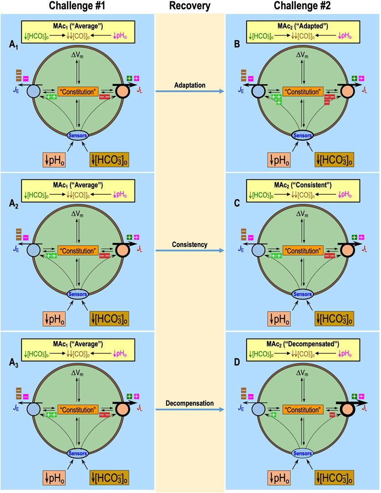
Figure 12. Model of the mechanisms of behavior. (A₁–A₃) Cell state during challenge #1. (A₁–A₃) These are identical and reflect the state of an “average” naïve HC neuron during the first challenge with MAc. After this MAc₁ challenge, the neuron spends several minutes in a recovery period, exposed to a control CO₂/HCO₃⁻ solution. The thicknesses of arrows for J_E (rate of acid loading from all sources) and J_L (rate of acid extrusion from all sources) reflect functional activities (i.e., product of the protein number and intrinsic activity per protein). (B) State of an adapted neuron during a second MAc challenge. We hypothesize that during MAc₂, individual transporters, individual sensors, and cellular constitution have changed in such a way as to make (J_E–J_L) more positive than during MAc₁ and thereby reduce the magnitude of (ΔpH_i)₂ compared to (ΔpH_i)₁. (C) State of a consistent neuron during a second MAc challenge. We hypothesize that during MAc₂, the net effect on (J_E–J_L) is the same as during MAc₁ in panel A, although individual transporters, individual sensors, and cellular constitution may have changed. (D) State of a decompensated neuron during a second MAc challenge. We hypothesize that during MAc₂, individual transporters, individual sensors, and cellular constitution have changed in such a way as to make (J_E–J_L) more negative than during MAc₁ and thereby increase the magnitude of (ΔpH_i)₂ compared to (ΔpH_i)₁. The symbols have the same meanings, as detailed in the previous figures. The thickness of the arrows representing J_E and J_L and the thickness of the lines surrounding “Sensors” reflect the relative functional activities. The numbers of intracellular light-green “plus” symbols and red “minus” symbols reflect the degree of stimulation or inhibition by the Sensors and/or Constitution. Although we show equal numbers of intracellular light-green “plus” symbols and red “minus” symbols, it is really some combination of the two that reflects the relative degrees of transporter stimulation/inhibition by “Sensors” and/or “Constitution.”

Adaptation

Figures 12A1, B illustrate our model for how the three factors conspire to produce Δ(J_E–J_L) that is less negative during MAc₂ than during the earlier MAc₁. As implied by the presentation in the previous paragraph, a cell could achieve adaptation by increasing J_E from MAc₁ to MAc₂ without any change (or even a smaller decrease) in J_L, or a decrease in J_L without any change (or even a smaller increase) in J_E. In any case, MAc₂ elicits a smaller pH_i decrease than MAc₁—adaptation.

Consistency

Figures 12A2, C illustrate our model, showing how overall (J_E–J_L)—regardless of changes in individual components of J_E and J_L—remains approximately the same during MAc₂, as during MAc₁ so that (ΔpH_i)₂ ≅ (ΔpH_i)₁,—consistency.

Decompensation

Figures 12A3, D illustrate our model, showing how overall (J_E–J_L)—regardless of changes in individual components of J_E and J_L—decreases during MAc₂ compared to MAc₁. As a result, MAc₂ elicits a larger pH_i decrease than MAc₁,—decompensation.

pAc₂ and pMet↓₂

In our presentation of Figure 11, we observed that, in a population of naïve neurons, the sum of ΔpH_i values in pAc₁ and pMet↓₁ is approximately equal to MAc₁. Figure 13 illustrates an analogous analysis of pAc and pMet↓ but for neurons previously challenged in period #1 with MAc.

Figure 13

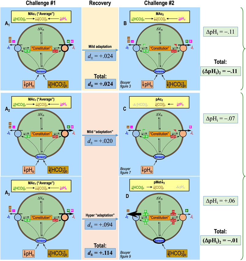
Figure 13. Model of the mechanism of non-additivity in MAc₁-treated neurons: pAc₂ + pMet↓₂ >> MAc₂. We hypothesize that MAc₁ produces the usual initial percent inhibition (extracellular brown or magenta “minus” symbols) or stimulation (extracellular dark-green or magenta “plus” symbols) of each transporter (see Figure 5E) and sensor (see Figure 6) and generates an average-sized pH_i decrease (see Figure 8). After the recovery period, we expose the cell either to MAc₂ panels (A₁–B), pAc₂ panels (A₂–C), or pMet↓₂ panels (A₃–D). The different behavior responses during challenge #2 would reflect differences in (1) transporter numbers, (2) sensor numbers, and (3) cellular constitution (which would influence intrinsic transporter and sensor activity). The symbols have the same meanings as detailed in the previous figures. The thickness of the arrows representing J_E (rate of acid loading from all sources) and J_L (rate of acid extrusion from all sources) and the thickness of the lines surrounding “Sensors” reflect the relative functional activities (i.e., product of the protein number and intrinsic activity per protein). Although we show equal numbers of intracellular light-green “plus” symbols and red “minus” symbols, it is really a combination of the two that reflects the relative degrees of transporter stimulation/inhibition by “Sensors” and/or “Constitution.” The d_± values are from table 2 of Bouyer et al. (2024). The “ΔpH_i” values in light-green boxes refer to challenge #2 and are obtained from the figure 3 panel (B), figure 7 panel (C), and figure 9 panel (D) of the same paper. The bolded “Total” values—either d_± or (ΔpH_i)₂—are either the same as for the single respective values in panel B or the sum of the two respective values for panels C and D. A₁–A₃, cell state during challenge #1. A₁, A₂, and A₃ are identical. MAc₁ produces a negative shift in Δ(J_E–J_L) and, therefore, a pH_i decrease, which is greater in magnitude than in panels B, C, or D. (B) Average response to MAc₂. We hypothesize that some combination of increased J_E and decreased J_L produces a modestly negative Δ(J_E–J_L) that is smaller in magnitude than during MAc₁. As a result, Δ(pH_i)_2/MAc has a smaller magnitude than (ΔpH_i)_1/MAc—a mild adaptation. (C) Average response to pAc₂. We hypothesize that some combination of increased J_E and decreased J_L produces a modestly negative Δ(J_E–J_L) that—as is the case in panel B—is smaller in magnitude than during MAc₁. As a result, Δ(pH_i)_2/pAc has a smaller magnitude than (ΔpH_i)_1/MAc—a mild “adaptation.” (D) Average response to pMet↓₂. We hypothesize that some combination of increased J_E and decreased J_L produces a massively positive Δ(J_E–J_L). As a result, Δ(pH_i)_2/pMet↓ is frankly positive—a “hyper adaptation.”

Non-additivity of pAc₂ and pMet↓₂ during MAc–MAc

Figures 13A1, B show cellular models of the average MAc–MAc data in figure 3 of Bouyer et al. (2024), who reported a mild decrease in ΔpH_i from MAc₁ (−0.14) to MAc₂ (−0.11) in concert with a modestly positive d_± (+0.024). In Figure 13B, we model this mild adaptation by adding a “half-plus” for J_E and a “half-minus” for J_L. Many combinations of J_E and J_L changes—produced by changes in the three factors¹³—could have elicited the required modest increase in (J_E–J_L).

Figures 13A2, C show models of the acidosis part of that MAc₂. Because in figure 7 of Bouyer et al. (2024), the (ΔpH_i)_1/MAc value was smaller (−0.11) than that in their figure 3 (−0.14), we interpret (ΔpH_i)_2/pAc (−0.07) as representing the 0MAc-pAc equivalent of mild adaptation. The d_± value of figure 7 (+0.020) was similar to that of figure 3 (+0.024). Therefore, we model pAc₂ in Figure 13C similarly to MAc₂ in Figure 13B, with an addition of a half-plus to J_E and half-minus to J_L. Our interpretation of Bouyer et al. (2024) data is that the stimulation of pH_o sensors by pAc₂ provides all the impetus necessary to produce the usual changes observed during MAc₂ of a MAc–MAc protocol; in other words, no input from HCO₃⁻ sensors is necessary to account for (ΔpH_i)_2/MAc.

Figures 13A3, D show models of the ↓[HCO₃⁻]_o part of that MAc₂. A note of caution: figure 9 of Bouyer et al. (2024) reports that (ΔpH_i)_1/MAc was smaller (−0.07) than both the population average (−0.11 in their figure 1) and the value reported in figure 3 (−0.14). Nevertheless, (ΔpH_i)₂ during pMet↓₂ is notably striking: an average pH_i increase of +0.06 with ∼87% of all neurons exhibiting a net pH_i increase during pMet↓₂ of the MAc-pMet↓ protocol. Thus, we are dealing with a strong phenotype. Furthermore, we recall that in naïve neurons, pMet↓₁ produced the smallest recorded average pH_i decrease (−0.04) and nearly 40% of the neurons underwent a frank pH_i increase (see their figure 8). Returning to Bouyer’s figure 9, d_± is also strikingly large (0.094). Thus, in evaluating the data underlying through CD, we reach similar conclusions whether we sum population ΔpH_i values (−0.07 + +0.06 = −0.01) or population d_± values (+0.020 + +0.094 = +0.114): in other words, the sum of the parts in panels C and D is far greater than the overall result in panel B ((ΔpH_i)₂ = −0.11, d_± = +0.024). How is this discrepancy possible?

We propose that HC neurons, during MAc₂ of a physiological MAc–MAc challenge, normally engage in coincidence detection involving two sets of acid–base sensors—one for extracellular H⁺ and another for extracellular HCO₃⁻. When the two challenges arrive with approximate simultaneity, their respective signal transduction cascades have the effect of muting one another, especially muting the strong actions of decreased [HCO₃⁻]_o during MAc₂.

Extreme paradoxical behavior pMet↓₂

In Figure 10, we proposed—knowing the pH_i responses to pMet↓₁ and pMet↓₂—that a small subset (∼10%) of naïve rat HC neurons respond to MAc₁ with an unbalanced activation of RPTPγ or RPTPζ, resulting in a paradoxical pH_i increase.

We propose that, also in naïve neurons, pMet↓₁—without accompanying muting contributed by decreased pH_o in MAc₁—produces an even more unbalanced net stimulation of acid extrusion. In nearly 40% of the population, this results in a paradoxical pH_i increase.

Finally, in HC neurons primed with an MAc₁ challenge and then allowed to recover, the subsequent exposure to pMet↓₂ produces the greatest unbalanced net increase in (J_E–J_L) such that ∼87% of Bouyer’s HC neurons exhibited a paradoxical pH_i increase. During/after MAc₁, the neuron does not “know” what the experimenter intends for the second challenge. MAc₁ and the subsequent recovery period must set the stage for the truly remarkable alkalinizing response (i.e., ↑pH_i) to pMet↓₂ in Bouyer’s figure 9. Bouyer likened this phenomenon to placing 100 glasses of room-temperature water into a functioning refrigerator, only to find that, after their removal, 87 glasses had warmed up (!).

MAc₂ in a normal MAc–MAc protocol

During MAc–MAc, one can view MAc₂—in a neuron that has already been preconditioned by MAc₁—as being pMet↓₂ (see Figure 13D) supplemented with pAc₂. We propose that the pAc₂ component—acting via ↓pH_o sensors like GPR68, ASICs, and TASKs (see Figure 6)—nullifies most of the alkalinizing effects of pMet↓₂ (Figure 14), an example of antagonism. Such H⁺-induced nullification may also occur to some extent in naïve neurons, and its variability could underlie some of the “state” variability observed in naïve neurons, as well as in those first challenged with MAc₁ and later subjected to MAc₂. See the legend of Figure 14 for a consideration of how our cartoon model is an oversimplification of the complexities of physiology. Refer to the section on mathematical modeling¹⁴ for suggestions on how to address these complexities.

Figure 14

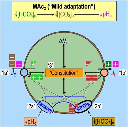
Figure 14. Revised mechanistic model of mild adaptation during MAc₂: coincidence detection. Inspired by the unique predictions in Figure 13D, we present this general model. We envisage that the response to MAc₂ represents more than the simple additivity of low-pH_o and low-[HCO₃⁻]_o stimuli, as depicted in Figure 13B. In this figure, we split the generic ↓pH_o/↓[HCO₃⁻]_o “Sensors” icon into separate sensors for ↓pH_o (‘2a’) and ↓[HCO₃⁻]_o (‘2b’). Although we retain the ability of the now-separate sensors—acting in parallel—to stimulate acid extrusion (‘1a’) and inhibit acid loading (‘1b’) and interact with “Constitution” (‘3’), we now introduce a new concept: the ↓pH_o sensors (‘2a’) must normally act during MAc₂ to antagonize the ↓[HCO₃⁻]_o sensor (‘2b’). Thus, we envisage that the sensors act in three ways: (1) pre-conditioned by MAc₁, the ↓[HCO₃⁻]_o sensors (e.g., RPTPγ and/or RPTPζ) are poised to produce—via actions of J_E, J_L, and Constitution—a massive increase in (J_E–J_L), which, by itself, would produce a paradoxical pH_i increase, as modeled in Figure 13D. Perhaps also pre-conditioned by MAc₁, the ↓pH_o sensors (e.g., GPR68) have two effects. (2) Parallel increase—via actions of J_E, J_L, and Constitution—in (J_E–J_L). (3) Massive inhibition of the response of the RPTPs to the low-[HCO₃⁻]_o stimulus. This model is a great oversimplification. The J_E (rate of acid loading from all sources) and J_L (rate of acid extrusion from all sources) icons represent a multitude of individual transporters. The sensors, although split into separate detectors of ↓pH_o and ↓[HCO₃⁻]_o, could represent multiple examples of each (see Figure 6). Constitution we defined as “the collection of all ion-concentration, metabolic, and signaling properties.” We envisage all of the individual effects to be time-dependent, both in terms of activation and deactivation (e.g., persistence). Dependencies of transporters, sensors, and enzymes on the concentrations of their relevant substrates/ligands are almost certainly nonlinear. When two arrows point at a target, the effects could be sub-additive, simply additive, or supra-additive (i.e., synergistic). The proposed inhibitory effect of the ↓pH_o on the ↓[HCO₃⁻]_o sensors is an example of antagonism. Assembling all of these complexities into a useful model is a task for mathematical modeling. Although we show equal numbers of intracellular light-green “plus” symbols and red “minus” symbols, it is really some combination of the two that reflects the relative degrees of transporter stimulation/inhibition by “Sensors” and/or “Constitution.”

Parameters’ potentially governing behavior

Not addressed in the studies of Salameh et al. (2014) and Bouyer et al. (2024) are several important unresolved questions regarding the duration of events required for establishing behaviors:

• Challenge #1: How does the development of a behavior depend on challenge #1, particularly its:

o nature (e.g., MAc₁ vs. pMet↓₁)?

o intensity (e.g., degree of lowering pH_o or [HCO₃⁻]_o)?

o duration?

• Recovery-period duration: How does the development of a particular behavior depend on the duration of the interlude period between challenges #1 and #2? The answer could depend on

o Preceding challenge #1 (nature, intensity, and duration)

o Challenge #2 (nature and intensity)

• Extinguishment: Over what duration of recovery period would the behavior-inducing effects of challenge #1 extinguish? The answer could depend on

o Preceding challenge #1 (duration, nature, and intensity)

o Challenge #2 (nature and intensity)

We suggest that a fruitful initial approach for addressing the abovementioned questions could be to use the MAc-pMet↓ protocol as a test case because it produces the most reproducible and remarkable responses. Recall that figure 9b in the study of Bouyer et al. (2024) shows that ∼87% of neurons subjected to this protocol exhibit a paradoxical pH_i increase.

It is of interest that, in the study of Bouyer et al. (2024) and the PhD dissertation of Taki (2024), the initial MAc₁-induced pH_i decrease (indicative of a negatively shifted [J_E–J_L]) was not followed by a delayed pH_i increase (reminiscent of adaptation) or pH_i decrease (reminiscent of decompensation) during MAc₁. Thus, we can conclude that either (1) the duration of challenge #1 (e.g., 7 min in the Taki study) was too brief for the development of a secondary change in (J_E–J_L) or (2) the removal of challenge #1 is necessary for the development of the behavior observed during challenge #2.

Although we have primarily focused on acid–base parameters as potential modulators of behavior, other environmental factors—metabotropic signaling molecules and the ionic milieu (e.g., [K⁺]_o)—also could also be in play.

Summary

At the population level, the behavior evidenced during MAc₂ is quite different from the simple sum of pAc₂ and pMet↓₂. Behavior could depend on the nature, intensity, and duration of challenge #1, as well as the duration of the recovery period. The response to pMet↓₂, perhaps mediated by RPTPγ/ζ, is extremely powerful, capable of producing rather consistent paradoxical increases in pH_i.

Impact on extracellular buffering

Resistant state and adaptation

Both a relatively resistant state and an adaptive behavior could be the appropriate “selfish” response of neurons, for which a relatively large acidic pH_i shift would have a negative impact on the physiological role of analogous neurons in an intact brain. Such hypothetical neurons—those especially critical under a particular set of circumstances—may be programmed to reduce the magnitude of acidic shifts using the strategies outlined above. The price to pay for such selfishness is that the cell’s small negative (J_E–J_L) necessarily results in the extrusion of acid into the extracellular space (see Figure 9C and Figure 12B), which lays an extra low-pH_o burden on neighboring cells.

Average state and consistency

Both an average¹⁰ state and a consistent behavior could be the appropriate “unselfish” response of neurons, for which an acidic pH_i shift would have a limited impact on the physiological role of an analogous neuron in an intact brain. By allowing themselves to acidify moderately during MAc₁ and/or to acidify no more during MAc₂ than during MAc₁, such neurons perform an important function by buffering extracellular acid and reducing extracellular acid loads experienced by neighboring cells.

Sensitive state and decompensation

Both a relatively sensitive state and a decompensating behavior could be the appropriate “altruistic” response of neurons, for which a relatively severe acidic pH_i shift would have limited impact on the physiological role of an analogous neuron in an intact brain. By allowing themselves to acidify to a relatively large degree during MAc₁, and/or acidifying more during MAc₂ than during MAc₁, these altruistic neurons buffer disproportionately greater fractions of extracellular acid loads and thereby spare their neighboring cells.

Astrocytes vs. neurons in the CNS

Although we have focused on neurons, it is interesting to recall that Salameh et al. (2014) found that, during a MAc–MAc protocol, ΔpH_i/ΔpH_o is consistently greater (by nearly 50%) for astrocytes than for neurons, both in cultures from the hippocampus and medullary raphé and both for MAc₁ and MAc₂. On the other hand, intrinsic intracellular buffering power (β_I; see Thornell et al. (2025) has the opposite pattern for the two cell types. For cultured astrocytes from rat HC, β_I is only ∼10 mM/pH at pH_i 7.0 in one study (Bevensee et al., 1997), whereas β_I of neurons acutely isolated from rat HC is much higher, ∼15 mM/pH at pH_i 7.0 in another study (Bevensee et al., 1996). Thus, if we consider only β_I, although their ΔpH_i may be 50% greater, HC astrocytes would take up about the same amount of acid per unit volume of cytosol as neurons. On the other hand, total intracellular buffering power (β_T) is the sum of β_I and the open-system CO₂/HCO₃⁻ buffering power (β_open), with the latter increasing exponentially¹⁵ with pH_i and being the same in all cells. Thus, at relatively low pH_i values, β_T would be modestly lower in astrocytes than in neurons, and astrocytes (with a 50% greater ΔpH_i) would buffer modestly more acid than neurons. At relatively high pH_i values, β_open would overwhelm β_I, and thus, β_T would be rather similar in the two cell types; in this case, astrocytes would buffer much more acid than neurons. Because astrocytes can undergo rather large pH_i changes and buffer more acid than neurons on average, we could view them as being altruistic compared to neurons.

Variability among neuronal responses

pH sensitivity of neurons

Changes in pH_o or pH_i can affect a wide range of electrophysiological properties because of the pH_i/pH_o sensitivity of virtually every neuronal component—including channels, receptors, transporters, enzymes (including those involved in neurotransmitter metabolism), and cytoskeletal elements. Thus, one would expect that inappropriate pH_i changes could lead to CNS pathology. It is generally believed that high neuronal pH_i is pro-epileptogenic (Hentschke et al., 2006; Jacobs et al., 2008; Sinning et al., 2011). Chesler and Kraig (1987), Chesler and Kraig (1989) and Ransom (2000) proposed a negative-feedback model, which was discussed and extended by Salameh et al. (2017). In this model, neuronal activity leads to an increase in [K⁺]_o, causing depolarization-induced alkalinization (DIA) in astrocytes (Siebens and Boron, 1989a; Siebens and Boron, 1989b), that in turn would cause a fall in pH_o—a local MAc—and, thus, a generalized reduction in neuronal excitability. We would expect that local MAc would lower neuronal pH_i. Induced epileptiform activity lowers neuronal pH_i, which recovers after the epileptiform activity ceases (Xiong et al., 2000; Raimondo et al., 2012). Although high pH_o is also considered to be pro-epileptogenic, chronic low-grade metabolic acidosis may contribute to the development of chronic epilepsy (Yuen, 2006).

Based on the above discussion, one might have expected the distribution of neuronal pH_i values to be within a relatively narrow range. However, a striking characteristic of mammalian HC neurons, freshly dissociated or cultured, is an unusually wide range of resting pH_i values (Schwiening and Boron, 1994; Baxter and Church, 1996; Bevensee et al., 1996; Smith et al., 1998) compared to other cell types. Moreover, our laboratory has identified a wide range of ΔpH_i responses to MAc (Bouyer et al., 2004; Salameh et al., 2014; 2017) and twin MAc–MAc challenges (Salameh et al., 2014; 2017). Bouyer et al. (2024) study confirms this diversity of responses to MAc (state) and MAc–MAc (behavior) and extends both aspects of diversity to the artificial acid–base disturbances pAc and pMet↓, alone and in combination with MAc.

Origin of pH_i diversity in neurons

We have already presented hypotheses to address the molecular mechanisms underlying the diversity of state and behavior. We now ask, at a higher level, what is responsible for the aforementioned diversity? We offer four possibilities that are not mutually exclusive.

(1) Some of the diversity is unphysiological. For example, the above-cited studies show that the broad range of initial pH_i values is greater in the absence than in the presence of CO₂/HCO₃⁻ (which would presumably enable the full complement of pH_i-regulatory mechanisms). It is possible that the range would be narrower still if we were to study the neurons in vivo, where they would be under the potential influence of metabotropic signaling and other influences from neighboring cells in a three-dimensional arrangement.

(2) Some of the acid–base diversity represents a diversity of neuronal subtypes, with each subtype, as studied in primary culture, having its own range of expressions for each relevant protein.

(3) Some of the diversity is intrinsic to neuronal physiology (nature), at least in primary culture, reflecting apparently stochastic differences in the numbers and localization of various proteins.

(4) Some of the diversity depends on the history of individual neurons (nurture), including differences in the acid–base microenvironment, patterns of neuronal activity, and other environmental parameters (e.g., cell–cell contacts) for these cells in primary culture.

Thus, each neuron in culture could have a set of properties that depends on neuronal subtype, stochastic variations in protein numbers/localization within that subtype (nature), and differences in neuronal history (nurture). Together, these factors could establish a constitution that determines how a particular neuron responds to one acid–base challenge (state) or a sequence of them (behavior).

Impact on cell function

A teleological question that arises is why should such diversity exist? One advantage of diversity could be to increase the probability that enough neurons in a circuit can withstand periodic acid–base challenges of various types. Another could be that neurons with different electrophysiological properties (and the underlying cohort of ion channels and other proteins, each with its own pH_i sensitivity) could be more electrically stable with a resistant vs. sensitive state or with an adaptive vs. consistent vs. decompensatory behavior.

Discussion

Major conclusions

Regarding the experiments with OOE solutions, we believe that the main conclusions of the paper by Bouyer et al. (2024) can be summarized as follows.

“State” during challenge #1

In a population of naïve rat HC neurons, the effects of pAc₁ and pMet↓₁ on pH_i—assessed as (ΔpH_i)₁—are approximately additive. In other words, in naïve HC neurons, whole MAc₁ is approximately the sum of its parts (see Figure 11).

Acid–base sensors

The abovementioned results lead to the conclusion that rat HC neurons have separate sensors that detect (1) a decrease in pH_o and (2) a decrease in [HCO₃⁻]_o (see Figure 6).

“Behavior” when challenge #1 is MAc₁

In a population of neurons that has already experienced MAc₁ followed by a recovery period, the subsequent effects of pAc₂ and pMet↓₂—as assessed by either (ΔpH_i)₂ or d_±—are decidedly not additive (see Figure 13).

Coincidence detection

The abovementioned result leads us to conclude that—for this protocol, which spans MAc₁ and a recovery period—pAc₂ and pMet↓₂ challenges must arrive at approximately the same time to reproduce the physiological effects of MAc₂ (see Figure 14).

Molecular mechanism

Mouse HC neurons express both RPTPγ and RPTPζ (Lorenzetto et al., 2014; Taki et al., 2024). Based on the PhD dissertation of Taki (2024), who examined the effect of knocking out RPTPζ in MAc–MAc and RAc–RAc protocols on mouse HC neurons, and the work of Zhou et al. (2016), who examined the effect of knocking out RPTPγ in renal proximal tubules, we propose that the most likely HCO₃⁻ sensor(s) in the experiments of Bouyer et al. (2024) are some combination of RPTPγ and RPTPζ.

In addition, we urge additional experiments that further probe the molecular mechanisms underlying state and behavior and suggest an extension of the studies to include (1) the duration and intensity of the first challenge, (2) the duration of the recovery period, and (3) additional acid–base challenges that involve both equilibrated solutions (i.e., RAc, MAlk, and RAlk) and OOE solutions (pAlk, pMet↑, pResp↓, and pResp↑).

Mathematical modeling

Aside from a call for more wet-laboratory data, we urge the development of mathematical models—the counterparts of the qualitative models described with words and cartoons in the present paper—that could assist in the interpretation of experiments like those in the research paper by Bouyer et al. (2024). Boron and De Weer (1976) developed the first mathematical model of pH_i regulation, a compartmental model that embodies the principles of the fundamental law of pH_i regulation in Equation 10. Occhipinti et al. (2020), as part of the Physiome journal (which is part of the broader Physiome Project), wrote a retrospective of the BDW model that includes clarifications and updates, access to online implementations, and a summary of several post-BDW models of pH_i regulation.

The set of two ordinary differential equations in the BDW model includes only one component of J_L (an H⁺ pump, the rate of which varies with [H⁺]_i—and thus time—according to a fixed rate constant) and a single component of J_E (an HCO₃⁻ leak, the rate of which varies with [HCO₃⁻]_i—and thus pH_i and time—according to a fixed HCO₃⁻ permeability). Although it would be straightforward to incorporate additional components of J_E (i.e., J_E1, J_E2, … ) and J_L (i.e., J_L1, J_L2, … ), imbuing these components (e.g., variants of NBCn1) with realistic estimates of sensitivity to pH_i and pH_o, as well as their respective substrates, would require major—but valuable—investments from funding agencies. The same applies to acid–base sensors and the broader issue of “cellular constitution,” which would describe diverse influences ranging from ion concentrations to signal transduction pathways.

Figure 14 is a cartoon model of how interactions among (1) transporters, (2) sensors, and (3) cellular constitution could account for the results of the recent study by Bouyer et al. (2024). As noted in the figure legend, the cartoon is greatly oversimplified: each transporter icon represents a multitude of individual proteins. The ↓pH_o and ↓[HCO₃⁻]_o sensors could represent multiple examples of each (see Figure 6). We defined constitution as “the collection of all ion-concentration, metabolic, and signaling properties.” All of the interconnected components vary with time during—and after—and acid–base challenge. Their dependencies on concentrations of their relevant substrates/ligands are almost certainly nonlinear. Effects could have varying degrees of additivity or antagonism.

A goal of programs such as The Physiome is to develop modular mathematical components for each transporter and signaling pathway, assemble the components into various model cells, and inform the models from experiments like those reported in the research paper by Bouyer et al. (2024). We envision the development of such sophisticated models—the quantitative versions of those qualitative models in the present paper—and using them to interpret the research paper by Bouyer et al. (2024) and design future experiments.

Limitations to the model(s)

We begin by acknowledging the principle that “all models are wrong, but some are useful”—the first part of which is articulated by the British statistician Box (1976), who also emphasized the concept of “useful.”

The word and cartoon models presented in this paper are based on the fundamental law of pH_i regulation (see Equation 10), which is mathematically expressed as follows:

$\frac{\mathit{d}{\text{pH}}_{\mathrm{i}}}{\text{dt}}=\frac{\mathit{\rho }}{\mathit{\beta }}\cdot \left({\mathit{J}}_{\mathrm{E}}-{\mathit{J}}_{\mathrm{L}}\right).(11)$

This equation is analogous to the principle of continuity in physiology¹⁶ or fluid mechanics, which, in turn, is based on the conservation of mass. Thus, the basic model must be correct, at least at the integrative level of classical physics and chemistry.

The theoretical cartoon models presented in this paper could be tested by employing more sophisticated mathematical modeling approaches than that explained in Equation 10. These approaches could resort to “compartmental” models, treating the cell and the extracellular fluid as uniform compartments with instantaneous mixing (i.e., ignoring a detailed spatial description of the cell geometry and its effects on solute diffusion). More complex approaches could resort to 3D (“distributed”) reaction-diffusion models, in which one accounts for the diffusion (or transport) of solutes in 3D space/time, as well as the chemical reactions that occur in parallel 3D space/time. For example, such models can attempt to account for unconvected layers that surround a cell and how geometry impacts the time courses of solute concentrations. In either case, the modeler formulates the problem using differential equations and solves these using various numerical methods. Assumptions—and opportunities for error—abound at each conceptual step.

Limitations also arise in the complexity of the biological system and the oversimplifications by which we estimate individual terms, even in the relatively simplest of approaches (e.g., a compartmental system):

Surface-to-volume ratio (ρ)

Although distributed mathematical models can describe complex cell geometries explicitly, they face increasing computational challenges when solving numerically the resulting (partial) differential equations. Generally, whenever possible, modelers overcome this challenge by simplifying cellular geometry, assuming that a cell has a simple geometric shape (e.g., a sphere or a cylinder). In the case of the oocyte models of Somersalo et al. (2012) and Occhipinti et al. (2014), the authors took advantage of the oocyte’s being a spherical cell and further simplified the model by assuming spherical radial symmetry (i.e., only the distance from the cell center influences solute transients). Occhipinti et al. (2014) incorporated an amplification of the surface area to accommodate microvilli. Even so, the volumes and surface areas of living cells are not precisely known, and they can change with time.

Buffering power (β)

Modelers might break buffering into two components: open-system buffering power (due to a solute like CO₂ or NH₃ that can equilibrate across the cell membrane) and intrinsic buffering power (Boron, 1977). As discussed by Thornell et al. (2025), the intrinsic buffering power (βI) of the cytosol comprises chemical buffering (due to classic acid–base equilibria), biochemical buffering (due to other reactions that consume/generate H⁺), and organellar buffering (due to the movement of H⁺ equivalents across organellar membranes). Although it may be reasonably straightforward to account for open-system buffering, βI is, in principle, extraordinarily complicated because myriad components contribute to it, and this could change with time and metabolic state. In addition, intrinsic buffering power is pH_i-sensitive—although it is possible to measure this, as first done by Boron (1977). The modeler might assume a constant/fixed βI, a constant pH_i-dependent βI, or—as done by Somersalo et al. (2012) and Occhipinti et al. (2014)—represent βI with a single chemical buffer pair (HA $\rightleftharpoons$ H⁺ + A^–) using a pK and total concentration chosen to mimic the cell buffering power. All of the above represent limitations to models.

Acid extrusion (J_E) and acid loading (J_L)

As noted in our discussion during the introduction of Equation 10, the overall J_E and J_L each comprise a multitude of different transporters (see Figure 3), each with a distinct set of kinetic parameters. To the best of our knowledge, not even one acid–base transporter is fully described kinetically. Thus, modelers are left to estimate the parameter values—a further limitation to quantitative models. The numbers and activities of the individual J_E/J_L components are likely to change with time and acid–base challenges like those discussed in the present paper—further limiting models.

Extracellular acid–base sensors

In Figure 6, we introduced several classes of extracellular acid–base sensors, of which we know of several pH_o-sensitive GPCRs (for review, see Thornell et al., 2025), pH-sensitive ion channels like ASICs and TASKs, and two CO₂/HCO₃⁻-sensitive RPTPs, each with several variants. GPCRs and RPTPs could each modulate individual acid–base transporters, probably as the result of complex signal transduction cascades. GPCRs and RPTPs could also modulate pH_o-sensitive channels like ASICs and TASKs and a myriad of other cellular processes that constitute cellular constitution. We do not fully understand the role of any one of the above in modulating pH_i homeostasis. All of the above uncertainty contributes to the limitations to models.

Cellular constitution

We defined cellular constitution as “the collection of all [intracellular] ion-concentration, metabolic, and signaling properties” that can directly impact (1) the transporters directly responsible for J_E and J_L and (2) extracellular acid–base sensors. This catch-all grouping of constantly changing (1) small inorganic and organic molecules and (2) peptides and other polymers (including proteins and nucleic acids) will be a major challenge to characterize. Liquid–liquid phase separations may be the loci of many important biochemical processes. The extensive uncertainty about all of the above processes contributes to model limitations.

Although the preceding discussion may seem discouraging, we are optimistic that—over the decades—a continuous effort by cellular physiologists will enable them to develop and inform models that—although “wrong”—become increasingly more “useful” in interpreting data and formulating further hypotheses (to be tested experimentally).

Data availability statement

Publicly available datasets were analyzed in this study. These data can be found here: in the companion paper.

Author contributions

PB: conceptualization, methodology, validation, writing–original draft, and writing–review and editing. RO: conceptualization, validation, writing–review and editing. ST: conceptualization and writing–review and editing. FM: conceptualization and writing–review and editing. WB: conceptualization, formal analysis, funding acquisition, methodology, project administration, writing–original draft, and writing–review and editing.

Funding

The author(s) declare that financial support was received for the research, authorship, and/or publication of this article. This work was supported by NIH grants NS 18400 and DK128315 and program project grant P01-HD32573 (PI: Gabriel Haddad). WB’s and FM’s contributions to this work were supported in part by the Department of Defense, Air Force Research Laboratory 711th Human Performance Wing, Studies and Analysis funding 22-012.

Acknowledgments

WB gratefully acknowledges the support of the Myers/Scarpa endowed chair. PB thanks the Valparaiso Summer Research Fellowship for its support in the elaboration of this manuscript.

Conflict of interest

The authors declare that the research was conducted in the absence of any commercial or financial relationships that could be construed as a potential conflict of interest.

Publisher’s note

All claims expressed in this article are solely those of the authors and do not necessarily represent those of their affiliated organizations, or those of the publisher, the editors and the reviewers. Any product that may be evaluated in this article, or claim that may be made by its manufacturer, is not guaranteed or endorsed by the publisher.

Footnotes

¹By acute, we loosely mean a few seconds to minutes. Over a period of hours, genomic responses to acid–base disturbances could involve other signaling pathways.

²See the section titled “State & Behavior.”

³We refer to figures, tables, equations, and named solutions in the 2024 Bouyer paper in italics, using all lowercase letters.

⁴Bouyer et al. (2024) chose this pMet↓ nomenclature to make room for a future “pMet↑” solution, in which [HCO₃⁻]_o would increase at a fixed [CO₂]_o and pH_o.

⁵As embodied in Equation, ρ and β influence the rate at which pH_i changes during extracellular acid–base disturbances but not the direction of the pH_i change or even steady-state pH_i.

⁶In the Discussion of that paper, see the section titled “Effects of acid–base challenges on [CO₃⁼]_o.”

⁷See “Determinants of neuronal state and behavior.”

⁸Here, we consider acute effects with a duration of minutes. If the challenges were to persist long enough, changes in protein synthesis could affect the quantity and identity of expressed proteins.

⁹See “Molecular basis … ”).

¹⁰We will use “average cell” in two closely related ways to denote a cell with a ΔpH_i, that is (1) the mean value for the population and (2) near the boundary between “resistant” and “sensitive” states, as shown in Figure 8.

¹¹See inline heading “Paradoxical responses.”

¹²Note that we make no statement about how the challenge affects the magnitudes or even the directions of the shifts in J_E vs. pH_i or J_L vs. pH_i (see Figures 8B, C) or the time courses of these shifts. We only require that the negative Δ(J_E–J_L), integrated over the period of the MAc challenge, produces (in this case) a “moderate” net intracellular acid load, resulting in a moderate decrease in pH_i. For example, one could imagine a situation in which MAc caused J_L to paradoxically increase but caused J_E to increase even more. Because Δ(J_E–J_L) < 0, pH_i would still decrease.

¹³(1) Identity and numbers of acid–base transporters in the plasma membrane, (2) extracellular acid–base sensors, and (3) cellular constitution. See “Molecular basis of effects of extracellular acid–base disturbances.”

¹⁴See “Discussion” > “Mathematical modeling.”

¹⁵β_open = 2.3 × [HCO₃⁻]_i = 2.3 × [HCO₃⁻]_o × 10^(pH_i–pHo).

¹⁶For example, the rate at which the volume of the chamber changes is determined by the difference between the blood inflow and blood outflow. If chamber volume is constant, then inflow must equal outflow.

References

Alvarez de la R., Krueger S. R., Kolar A., Shao D., Fitzsimonds R. M., Canessa C. M. (2003). Distribution, subcellular localization and ontogeny of ASIC1 in the mammalian central nervous system. J. Physiology 546, 77–87. doi:10.1113/jphysiol.2002.030692

CrossRef Full Text | Google Scholar

Baxter K. A., Church J. (1996). Characterization of acid extrusion mechanisms in cultured fetal rat hippocampal neurones. J. Physiol. (Lond.) 493 (Pt 2), 457–470. doi:10.1113/jphysiol.1996.sp021396

PubMed Abstract | CrossRef Full Text | Google Scholar

Bevensee M. O., Bashi E., Schlue W. R., Boyarsky G., Boron W. F. (1999). Shrinkage-induced activation of Na⁺/H⁺ exchange in rat renal mesangial cells. Am. J. Physiol. 276, C674–C683. doi:10.1152/ajpcell.1999.276.3.C674

PubMed Abstract | CrossRef Full Text | Google Scholar

Bevensee M. O., Boron W. F. (2013). “Control of intracellular pH,” in Seldin and giebisch’s the kidney: physiology and pathophysiology (Academic Press), 1773–1835.

Google Scholar

Bevensee M. O., Cummins T. R., Haddad G. G., Boron W. F., Boyarsky G. (1996). pH regulation in single CA1 neurons acutely isolated from the hippocampi of immature and mature rats. J. Physiol. (Lond) 494, 315–328. doi:10.1113/jphysiol.1996.sp021494

PubMed Abstract | CrossRef Full Text | Google Scholar

Bevensee M. O., Weed R. A., Boron W. F. (1997). Intracellular pH regulation in cultured astrocytes from rat hippocampus. I. Role of HCO₃⁻. J. Gen. Physiol. 110, 453–465. doi:10.1085/jgp.110.4.453

PubMed Abstract | CrossRef Full Text | Google Scholar

Boron W. F. (1977). Intracellular pH transients in giant barnacle muscle fibers. Am. J. Physiol. 233, C61–C73. doi:10.1152/ajpcell.1977.233.3.C61

PubMed Abstract | CrossRef Full Text | Google Scholar

Boron W. F. (1985). Intracellular pH-regulating mechanism of the squid axon. Relation between the external Na⁺ and HCO₃⁻ dependences. J. Gen. Physiol. 85, 325–345. doi:10.1085/jgp.85.3.325

PubMed Abstract | CrossRef Full Text | Google Scholar

Boron W. F. (2004). Regulation of intracellular pH. Adv. Physiol. Educ. 28, 160–179. doi:10.1152/advan.00045.2004

PubMed Abstract | CrossRef Full Text | Google Scholar

Boron W. F. (2017). “Acid-base physiology,” in Medical physiology: a cellular and molecular approach. Editors W. F. Boron, and E. L. Boulpaep (Philadelphia, PA: Saunders Elsevier), 628–646.

Google Scholar

Boron W. F., Boulpaep E. L. (1983). Intracellular pH regulation in the renal proximal tubule of the salamander. Basolateral HCO₃⁻ transport. J. Gen. Physiol. 81, 53–94. doi:10.1085/jgp.81.1.53

PubMed Abstract | CrossRef Full Text | Google Scholar

Boron W. F., De Weer P. (1976). Intracellular pH transients in squid giant axons caused by CO2, NH3, and metabolic inhibitors. J. Gen. Physiol. 67, 91–112. doi:10.1085/jgp.67.1.91

PubMed Abstract | CrossRef Full Text | Google Scholar

Boron W. F., Knakal R. C. (1989). Intracellular pH-regulating mechanism of the squid axon. Interaction between DNDS and extracellular Na⁺ and HCO₃⁻. J. Gen. Physiol. 93, 123–150. doi:10.1085/jgp.93.1.123

PubMed Abstract | CrossRef Full Text | Google Scholar

Boron W. F., Knakal R. C. (1992). Na⁺-dependent Cl⁻-HCO₃⁻ exchange in the squid axon. Dependence on extracellular pH. J. Gen. Physiol. 99, 817–837. doi:10.1085/jgp.99.5.817

PubMed Abstract | CrossRef Full Text | Google Scholar

Boron W. F., Russell J. M. (1983). Stoichiometry and ion dependencies of the intracellular-pH-regulating mechanism in squid giant axons. J. Gen. Physiol. 81, 373–399. doi:10.1085/jgp.81.3.373

PubMed Abstract | CrossRef Full Text | Google Scholar

Bouyer P., Bradley S. R., Zhao J., Wang W., Richerson G. B., Boron W. F. (2004). Effect of extracellular acid-base disturbances on the intracellular pH of neurones cultured from rat medullary raphe or hippocampus. J. Physiol. (Lond.) 559, 85–101. doi:10.1113/jphysiol.2004.067793

PubMed Abstract | CrossRef Full Text | Google Scholar

Bouyer P., Zhou Y., Boron W. F. (2003). An increase in intracellular calcium concentration that is induced by basolateral CO₂ in rabbit renal proximal tubule. Am. J. Physiol. Ren. Physiol. 285, F674–F687. doi:10.1152/ajprenal.00107.2003

PubMed Abstract | CrossRef Full Text | Google Scholar

Bouyer P. G., Salameh A. I., Zhou Y., Kolba T. N., Boron W. F. (2024). Effects of extracellular metabolic acidosis and out-of-equilibrium CO₂/HCO₃⁻ solutions on intracellular pH in cultured rat hippocampal neurons. Front. Physiol. 15, 1434359. doi:10.3389/fphys.2024.1434359

PubMed Abstract | CrossRef Full Text | Google Scholar

Box G. E. P. (1976). Science and statistics. J. Am. Stat. Assoc. 71, 791–799. doi:10.1080/01621459.1976.10480949

CrossRef Full Text | Google Scholar

Brett C. L., Kelly T., Sheldon C., Church J. (2002). Regulation of Cl⁻/HCO₃⁻ exchangers by cAMP-dependent protein kinase in adult rat hippocampal CA1 neurons. J. Physiol. (Lond.) 545, 837–853. doi:10.1113/jphysiol.2002.027235

PubMed Abstract | CrossRef Full Text | Google Scholar

Chen J., Martinez J., Milner T. A., Buck J., Levin L. R. (2013). Neuronal expression of soluble adenylyl cyclase in the mammalian brain. Brain Res. 1518, 1–8. doi:10.1016/j.brainres.2013.04.027

PubMed Abstract | CrossRef Full Text | Google Scholar

Chen Y., Cann M. J., Litvin T. N., Iourgenko V., Sinclair M. L., Levin L. R., et al. (2000). Soluble adenylyl cyclase as an evolutionarily conserved bicarbonate sensor. Science 289, 625–628. doi:10.1126/science.289.5479.625

PubMed Abstract | CrossRef Full Text | Google Scholar

Chesler M., Kraig R. P. (1987). Intracellular pH of astrocytes increases rapidly with cortical stimulation. Am. J. Physiol. Regul. Integr. Comp. Physiol. 253, R666–R670. doi:10.1152/ajpregu.1987.253.4.R666

PubMed Abstract | CrossRef Full Text | Google Scholar

Chesler M., Kraig R. P. (1989). Intracellular pH transients of mammalian astrocytes. J. Neurosci. 9, 2011–2019. doi:10.1523/JNEUROSCI.09-06-02011.1989

PubMed Abstract | CrossRef Full Text | Google Scholar

Davis B. A., Hogan E. M., Boron W. F. (1994). Shrinkage-induced activation of Na⁺-H⁺ exchange in barnacle muscle fibers. Am. J. Physiology - Cell Physiology 266, C1744–C1753. doi:10.1152/ajpcell.1994.266.6.C1744

PubMed Abstract | CrossRef Full Text | Google Scholar

Hayashi N., Oohira A., Miyata S. (2005). Synaptic localization of receptor-type protein tyrosine phosphatase zeta/beta in the cerebral and hippocampal neurons of adult rats. Brain Res. 1050, 163–169. doi:10.1016/j.brainres.2005.05.047

PubMed Abstract | CrossRef Full Text | Google Scholar

Hentschke M., Wiemann M., Hentschke S., Kurth I., Hermans-Borgmeyer I., Seidenbecher T., et al. (2006). Mice with a targeted disruption of the Cl⁻/HCO₃⁻ exchanger AE3 display a reduced seizure threshold. Mol. Cell. Biol. 26, 182–191. doi:10.1128/MCB.26.1.182-191.2006

PubMed Abstract | CrossRef Full Text | Google Scholar

Hogan E. M., Davis B. A., Boron W. F. (1997). Intracellular Cl⁻ dependence of Na-H exchange in barnacle muscle fibers under normotonic and hypertonic conditions. J. Gen. Physiol. 110, 629–639. doi:10.1085/jgp.110.5.629

PubMed Abstract | CrossRef Full Text | Google Scholar

Horiguchi K., Higuchi M., Yoshida S., Nakakura T., Tateno K., Hasegawa R., et al. (2014). Proton receptor GPR68 expression in dendritic-cell-like S100β-positive cells of rat anterior pituitary gland: GPR68 induces interleukin-6 gene expression in extracellular acidification. Cell Tissue Res. 358, 515–525. doi:10.1007/s00441-014-1958-x

PubMed Abstract | CrossRef Full Text | Google Scholar

Huang W. C., Swietach P., Vaughan-Jones R. D., Ansorge O., Glitsch M. D. (2008). Extracellular acidification elicits spatially and temporally distinct Ca²⁺ signals. Curr. Biol. 18, 781–785. doi:10.1016/j.cub.2008.04.049

PubMed Abstract | CrossRef Full Text | Google Scholar

Imber A. N., Santin J. M., Graham C. D., Putnam R. W. (2014). A HCO₃⁻-dependent mechanism involving soluble adenylyl cyclase for the activation of Ca²⁺ currents in locus coeruleus neurons. Biochim. Biophys. Acta 1842, 2569–2578. doi:10.1016/j.bbadis.2014.07.027

PubMed Abstract | CrossRef Full Text | Google Scholar

Jacobs S., Ruusuvuori E., Sipilä S. T., Haapanen A., Damkier H. H., Kurth I., et al. (2008). Mice with targeted Slc4a10 gene disruption have small brain ventricles and show reduced neuronal excitability. Proc. Natl. Acad. Sci. U.S.A. 105, 311–316. doi:10.1073/pnas.0705487105

PubMed Abstract | CrossRef Full Text | Google Scholar

Lamprianou S., Vacaresse N., Suzuki Y., Meziane H., Buxbaum J. D., Schlessinger J., et al. (2006). Receptor protein tyrosine phosphatase γ is a marker for pyramidal cells and sensory neurons in the nervous system and is not necessary for normal development. Mol. Cell. Biol. 26, 5106–5119. doi:10.1128/MCB.00101-06

PubMed Abstract | CrossRef Full Text | Google Scholar

Lee S.-K., Occhipinti R., Moss F. J., Parker M. D., Grichtchenko I. I., Boron W. F. (2023). Distinguishing among HCO₃⁻, CO₃⁼, and H⁺ as substrates of proteins that appear to be “bicarbonate” transporters. J. Am. Soc. Nephrol. 34, 40–54. doi:10.1681/ASN.2022030289

PubMed Abstract | CrossRef Full Text | Google Scholar

Lesage F. (2003). Pharmacology of neuronal background potassium channels. Neuropharmacology 44, 1–7. doi:10.1016/s0028-3908(02)00339-8

PubMed Abstract | CrossRef Full Text | Google Scholar

Lorenzetto E., Moratti E., Vezzalini M., Harroch S., Sorio C., Buffelli M. (2014). Distribution of different isoforms of receptor protein tyrosine phosphatase γ (Ptprg-RPTP γ) in adult mouse brain: upregulation during neuroinflammation. Brain Struct. Funct. 219, 875–890. doi:10.1007/s00429-013-0541-7

PubMed Abstract | CrossRef Full Text | Google Scholar

Michenkova M., Taki S., Blosser M. C., Hwang H. J., Kowatz T., Moss F. J., et al. (2021). Carbon dioxide transport across membranes. Interface Focus 11, 20200090. doi:10.1098/rsfs.2020.0090

PubMed Abstract | CrossRef Full Text | Google Scholar

Moss F. J., Wass A. B., Watterson S. J., Boron W. F. (2018). Sensing and transduction of acid-base disturbances by receptor protein tyrosine phosphatase γ. FASEB J. 32, 864–865. doi:10.1096/fasebj.2018.32.1_supplement.864.5

CrossRef Full Text | Google Scholar

Müller S., Lamszus K., Nikolich K., Westphal M. (2004). Receptor protein tyrosine phosphatase ζ as a therapeutic target for glioblastoma therapy. Expert Opin. Ther. Targets 8, 211–220. doi:10.1517/14728222.8.3.211

PubMed Abstract | CrossRef Full Text | Google Scholar

Occhipinti R., Musa-Aziz R., Boron W. F. (2014). Evidence from mathematical modeling that carbonic anhydrase II and IV enhance CO₂ fluxes across Xenopus oocytes plasma membranes. Am. J. Physiol. Cell Physiol. 307, C841–C858. doi:10.1152/ajpcell.00049.2014

PubMed Abstract | CrossRef Full Text | Google Scholar

Occhipinti R., Safaei S., Hunter P., Boron W. F. (2020). The Boron and De Weer model of intracellular pH regulation. Physiome. doi:10.36903/physiome.12871022

CrossRef Full Text | Google Scholar

Parker J. C. (1983). Volume-responsive sodium movements in dog red blood cells. Am. J. Physiol. 244, C324–C330. doi:10.1152/ajpcell.1983.244.5.C324

PubMed Abstract | CrossRef Full Text | Google Scholar

Radu C. G., Nijagal A., McLaughlin J., Wang L., Witte O. N. (2005). Differential proton sensitivity of related G protein-coupled receptors T cell death-associated gene 8 and G2A expressed in immune cells. Proc. Natl. Acad. Sci. U. S. A. 102, 1632–1637. doi:10.1073/pnas.0409415102

PubMed Abstract | CrossRef Full Text | Google Scholar

Raimondo J. V., Irkle A., Wefelmeyer W., Newey S. E., Akerman C. J. (2012). Genetically encoded proton sensors reveal activity-dependent pH changes in neurons. Front. Mol. Neurosci. 5, 68. doi:10.3389/fnmol.2012.00068

PubMed Abstract | CrossRef Full Text | Google Scholar

Rajendran V. M., Geibel J., Binder H. J. (1995). Chloride-dependent Na-H exchange. A novel mechanism of sodium transport in colonic crypts. J. Biol. Chem. 270, 11051–11054. doi:10.1074/jbc.270.19.11051

PubMed Abstract | CrossRef Full Text | Google Scholar

Rajendran V. M., Geibel J., Binder H. J. (1999). Role of Cl channels in Cl-dependent Na/H exchange. Am. J. Physiology - Gastrointest. Liver Physiology 276, G73–G78. doi:10.1152/ajpgi.1999.276.1.G73

PubMed Abstract | CrossRef Full Text | Google Scholar

Ransom B. R. (2000). Glial modulation of neural excitability mediated by extracellular pH: a hypothesis revisited. Prog. Brain Res. 125, 217–228. doi:10.1016/S0079-6123(00)25012-7

PubMed Abstract | CrossRef Full Text | Google Scholar

Ransom B. R. (2017). “The neuronal microenvironment,” in Medical physiology: a cellular and molecular approach. Editors W. F. Boron, and E. L. Boulpaep (Philadelphia, PA: Saunders Elsevier), 275–294.

CrossRef Full Text | Google Scholar

Roos A., Boron W. F. (1981). Intracellular pH. Physiol. Rev. 61, 296–434. doi:10.1152/physrev.1981.61.2.296

PubMed Abstract | CrossRef Full Text | Google Scholar

Ruffin V. A., Taki S., Boron W. F., Moss F. J. (2025). Novel RPTPγ and RPTPζ splice variants from mixed neuron–astrocyte hippocampal cultures as well as from the hippocampi of newborn and adult mice. Front. Physiol. 15. doi:10.3389/fphys.2024.1406448

PubMed Abstract | CrossRef Full Text | Google Scholar

Salameh A. I., Hübner C. A., Boron W. F. (2017). Role of Cl⁻-HCO₃⁻ exchanger AE3 in intracellular pH homeostasis in cultured murine hippocampal neurons, and in crosstalk to adjacent astrocytes. J. Physiol. (Lond.) 595, 93–124. doi:10.1113/JP272470

PubMed Abstract | CrossRef Full Text | Google Scholar

Salameh A. I., Ruffin V. A., Boron W. F. (2014). Effects of metabolic acidosis on intracellular pH responses in multiple cell types. Am. J. Physiol. Regul. Integr. Comp. Physiol. 307, R1413–R1427. doi:10.1152/ajpregu.00154.2014

PubMed Abstract | CrossRef Full Text | Google Scholar

Schneider J. W., Goetsch S. C., Leng X., Ludwig S. M., Russell J. L., Yang C.-P., et al. (2012). Coupling hippocampal neurogenesis to brain pH through proneurogenic small molecules that regulate proton sensing G protein-coupled receptors. ACS Chem. Neurosci. 3, 557–568. doi:10.1021/cn300025a

PubMed Abstract | CrossRef Full Text | Google Scholar

Schwiening C. J., Boron W. F. (1994). Regulation of intracellular pH in pyramidal neurones from the rat hippocampus by Na⁺-dependent Cl⁻-HCO₃⁻ exchange. J. Physiol. (Lond) 475, 59–67. doi:10.1113/jphysiol.1994.sp020049

PubMed Abstract | CrossRef Full Text | Google Scholar

Siebens A. W., Boron W. F. (1989a). Depolarization-induced alkalinization in proximal tubules. I. Characteristics and dependence on Na⁺. Am. J. Physiol. 256, F342–F353. doi:10.1152/ajprenal.1989.256.2.F342

PubMed Abstract | CrossRef Full Text | Google Scholar

Siebens A. W., Boron W. F. (1989b). Depolarization-induced alkalinization in proximal tubules. II. Effects of lactate and SITS. Am. J. Physiol. 256, F354–F365. doi:10.1152/ajprenal.1989.256.2.F354

PubMed Abstract | CrossRef Full Text | Google Scholar

Sinning A., Liebmann L., Kougioumtzes A., Westermann M., Bruehl C., Hübner C. A. (2011). Synaptic glutamate release is modulated by the Na⁺-driven Cl⁻/HCO₃⁻ exchanger Slc4a8. J. Neurosci. 31, 7300–7311. doi:10.1523/JNEUROSCI.0269-11.2011

PubMed Abstract | CrossRef Full Text | Google Scholar

Smith G. A., Brett C. L., Church J. (1998). Effects of noradrenaline on intracellular pH in acutely dissociated adult rat hippocampal CA1 neurones. J. Physiol. (Lond.) 512 (Pt 2), 487–505. doi:10.1111/j.1469-7793.1998.487be.x

PubMed Abstract | CrossRef Full Text | Google Scholar

Somersalo E., Occhipinti R., Boron W. F., Calvetti D. (2012). A reaction-diffusion model of CO₂ influx into an oocyte. J. Theor. Biol. 309, 185–203. doi:10.1016/j.jtbi.2012.06.016

PubMed Abstract | CrossRef Full Text | Google Scholar

Taki S. (2024). Identification of novel murine RPTPγ and RPTPζ splice variants and the role of RPTPζ in modulating the neuronal and astrocytic intracellular pH response to metabolic or respiratory acidosis. Cleveland, OH: Case Western Reserve University Health Sciences. Available at: https://etd.ohiolink.edu/.

Google Scholar

Taki S., Boron W. F., Moss F. J. (2024). Novel RPTPγ and RPTPζ splice variants from mixed neuron-astrocyte hippocampal cultures as well as from the hippocampi of newborn and adult mice. Front. Physiol. 15, 1406448. doi:10.3389/fphys.2024.1406448

PubMed Abstract | CrossRef Full Text | Google Scholar

Thornell I. M., Michenkova M., Taki S., Bevensee M. O., Boron W. F. (2025). “Intracellular pH homeostasis,” in Seldin and giebisch’s the kidney: physiology and pathophysiology. Editors R. J. Alpern, M. J. Caplan, O. W. Moe, and S. E. Quaggin (London: Elsevier/Academic Press). Available at: https://www.barnesandnoble.com/w/seldin-and-giebischs-the-kidney-robert-j-alpern/1138252983 (Accessed August 29, 2023).

Google Scholar

Xiong Z. Q., Saggau P., Stringer J. L. (2000). Activity-dependent intracellular acidification correlates with the duration of seizure activity. J. Neurosci. 20, 1290–1296. doi:10.1523/JNEUROSCI.20-04-01290.2000

PubMed Abstract | CrossRef Full Text | Google Scholar

Yuen A. W. C. (2006). Low-grade chronic metabolic acidosis is a contributory mechanism in the development of chronic epilepsy. Epilepsy Behav. 8, 347–349. doi:10.1016/j.yebeh.2005.11.012

PubMed Abstract | CrossRef Full Text | Google Scholar

Zhao J., Hogan E. M., Bevensee M. O., Boron W. F. (1995). Out-of-equilibrium CO₂/HCO₃⁻solutions and their use in characterizing a new K⁺/HCO₃⁻ cotransporter. Nature 374, 636–639. doi:10.1038/374636a0

PubMed Abstract | CrossRef Full Text | Google Scholar

Zhao J., Zhou Y., Boron W. F. (2003). Effect of isolated removal of either basolateral HCO₃⁻ or basolateral CO₂ on HCO₃⁻ reabsorption by rabbit S2 proximal tubule. Am. J. Physiol. Ren. Physiol. 285, F359–F369. doi:10.1152/ajprenal.00013.2003

PubMed Abstract | CrossRef Full Text | Google Scholar

Zhou Y., Skelton L. A., Xu L., Chandler M. P., Berthiaume J. M., Boron W. F. (2016). Role of receptor protein tyrosine phosphatase γ in sensing extracellular CO₂ and HCO₃⁻. J. Am. Soc. Nephrol. 27, 2616–2621. doi:10.1681/ASN.2015040439

PubMed Abstract | CrossRef Full Text | Google Scholar

Zhou Y., Zhao J., Bouyer P., Boron W. F. (2005). Evidence from renal proximal tubules that HCO₃⁻ and solute reabsorption are acutely regulated not by pH but by basolateral HCO₃⁻ and CO₂. Proc. Natl. Acad. Sci. U.S.A. 102, 3875–3880. doi:10.1073/pnas.0500423102

PubMed Abstract | CrossRef Full Text | Google Scholar