 Oscar Alfredo Montenegro Arjona
 Jairo Montenegro Arjona
 Cristina Blasco Lafarga
 Ana Cordellat
- 1Physical Education and Sports Studies Programme, ALTIUS Research Group, Universidad Surcolombiana, Neiva, Colombia
- 2Mathematics Department, Universidad Nacional de Colombia, Bogotá, Colombia
- 3Sport Performance and Physical Fitness Research Group (UIRFIDE), Physical Education and Sport Department, University of Valencia, Valencia, Spain
A Commentary on
The polarization-index: a simple calculation to distinguish polarized from non-polarized training intensity distributions
by Treff G, Winkert K, Sareban M, Steinacker JM and Sperlich B (2019). Front. Physiol. 10:707. doi: 10.3389/fphys.2019.00707
Introduction
In a recent paper, Treff et al. (2019) discussed and presented the polarization index (PI), which allows us to distinguish if a training intensity distribution (TID) of endurance athletes is polarized; this is achieved when PI
Succinctly, TID quantification is classified based on exercise distribution over time or distance into three zones comprising the “intensity zone-model”: Zone 1 (low intensity), Zone 2 (threshold intensity), and Zone 3 (high intensity). The total exercise prescription (100%) is distributed into these three zones (i.e., Zone 1 + Zone 2 + Zone 3 = 100%).
A polarized TID is defined based on two conditions: (i) a polarized structure, that is, Zone 1
Discussion
We appreciate the establishment of PI and the cut-off
This comment aims to point out some underlying conditions and analysis in the use of Formulas (1) and (2) proposed by Treff et al. (2019), and their graphical interpretation, apart from giving a more compact functional notation for those formulas that allow easy transcription into scientific software.
About polarized TID conditions and the formulas
The three zones of an “intensity zone-model”, namely, Zone 1, Zone 2, and Zone 3, are denoted by z1, z2, and z3, respectively, and they are expressed in proportions instead of percentages. Regardless of units, this means that z1, z2, and z3 are real numbers in the interval [0,1] (i.e., 0 ≤ z1, z2, z3 ≤ 1) such that z1 + z2 + z3 = 1. The condition (i) for a polarized TID is 0 ≤ z2 < z3 < z1. The PI is made to capture the condition (ii).
This implies that PI calculation is only valid for TID that satisfies a polarized structure, that is, condition (i). Otherwise, we would be calculating the PI value of TID that does not meet condition (i), so it will never be a polarized TID independent of its PI.
From the aforementioned finding, if Zone 3 = 0, PI is zero per definition (Treff et al., 2019). In this case, we are dealing with TID that does not satisfy the polarized structure (condition (i)): it is not possible to have 0 ≤ z2 < 0 with some z2 in the interval [0,1]. However, the case z3 = 0 is not part of the cases, where we want to define PI.
Similarly, if Zone 3
In Treff et al. (2019), some calculations are performed in addition to the PI analysis. In particular, with the aim of explaining that two different TIDs (e.g., z1 = 0.90, z2 = 0.05, and z3 = 0.05 and z1 = 0.74, z2 = 0.13, and z3 = 0.13) can give the same result, PI = 2. This example leads to ambiguity because it does not meet condition (i), which is known as a polarized structure (0 < z2 and z2 < z3, and z3 < z1). However, if we want to calculate PI for these values, we have
and
These values are not equal to or close to 2.
Calculation of the polarization index
Given the importance of using PI in sports training and in support of the proposal by Treff et al. (2019), the PI calculation can be reformulated compactly and clearly as a piecewise function. In this sense, we propose a modification to Eqs (1) and (2) proposed by Treff et al. (2019). Our function contemplates all the conditions by applying a single measure, excluding those TID that were not necessary to calculate.
Given a TID based on a three-zone model, with measurements z1, z2, and z3 of Zone 1, Zone 2, and Zone 3, such that z1, z2, z3 ∈ [0, 1] and z1 + z2 + z3 = 1, we define PI as follows:
In other cases, PI is not defined.
The function PI defined in (1) makes explicit the adequate conditions on z1, z2, and z3 to obtain well-behaved Formulas (1) and (2), from Treff et al. (2019), on a more consistent and standard mathematical notation.
Polarization index: a cut-off
Herein, we want to determine if TID, which satisfies the condition (i), is polarized. Treff et al. (2019) proposed a cut-off for PI of 2: if PI ≤ 2, TID is non-polarized. The reasoning to reach this cut-off is based on the analysis of their Figure 2, which shows us a plot in two dimensions that attempt to capture the interactions of three fractions of the intensity zones, but Figure 2 is hard to interpret to follow the arguments proposed therein.
Taking into account that the function (1) proposed previously has its domain contained in a 3D space, that is, a set of points in the form (z1, z2, z3) that satisfy condition (i), a more accurate, easy to understand, and useful plot is shown in our Figure 1.
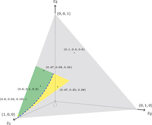
FIGURE 1. Domain of the PI function, a subset of a 3D space of points (z1, z2, z3), represented in green, blue, and yellow. These points satisfy condition (i). Green points represent PI(z1, z2, z3) > 2 (polarized TID), blue points (dashed line) represent PI(z1, z2, z3) = 2 (cut-off non-polarized TID), and yellow points represent PI(z1, z2, z3) < 2 (non-polarized TID). Gray points complete the set of points such that z1, z2, z3 ∈ [0, 1] and z1 + z2 + z3 = 1 (TID). Some points are tagged.
Implementing the polarization index
An implementation example of function (1) in scientific software is the following snippet code written in R programming language (R Core Team, 2021) using a couple of functions from the package dplyr, part of tidyverse (Wickham et al., 2019). The function implementation verifies all the hypotheses for TID and condition (i).
require(dplyr)
f_PI <– function(z1, z2, z3){
# First, verify the condition 0 <= z1, z2, z3 <=1 and z1 + z2 + z3 = 1
if(0 <= z1 & z1 <= 1 & 0 <= z2 & z2 <= 1 &
0 <= z3 & z3 <= 1 & dplyr::near(z1 + z2 + z3, 1)) {
# PI Piecewise function verify condition (i)
dplyr::case_when(
0 < z2 & z2 < z3 & z3 < z1 ∼ log10(100 * (z1/z2) * (z3)),
dplyr::near(z2, 0) & 0.01 < z3 & z3 < z1 ∼ log10(100 * (z1/0.01) * (z3-0.01)),
TRUE ∼ as.double(NA)) # TID does not meet condition (i)
} else {
# It is not a TID
as.double(NA)
}
}
Some example calculations
f_PI(0.6, 0.15, .25)
#> [1] 2
# *** Examples from Treff et al. (2019)
f_PI(0.6, 0.19, 0.21)
#> [1] 1.821617
f_PI(0.6, 0.14, 0.26)
#> [1] 2.046997
f_PI(0.8, 0.08, 0.12)
#> [1] 2.079181
f_PI(0.9, 0.05, 0.05)
#> [1] NA
f_PI(0.74, 0.13, 0.13)
#> [1] NA
# *** Some examples with z2 = 0
f_PI(1, 0, 0)
#> [1] NA
f_PI(0.99, 0, 0.01)
#> [1] NA
f_PI(0.9899, 0, 0.0101)
#> [1] -0.004408676
f_PI(0.9799, 0, 0.0201)
#> [1] 1.995503
f_PI(0.9701, 0, 0.0299)
#> [1] 2.165096
Author contributions
OM identified numerical errors and ambiguous conditions. OM, JM, CB, and AC contributed to the conception and design of the study. JM performed the mathematical analysis. OM and JM wrote the first draft of the manuscript. CB and AC wrote sections of the manuscript. All authors contributed to the article and approved the submitted version.
Conflict of interest
The authors declare that the research was conducted in the absence of any commercial or financial relationships that could be construed as a potential conflict of interest.
Publisher’s note
All claims expressed in this article are solely those of the authors and do not necessarily represent those of their affiliated organizations, or those of the publisher, the editors, and the reviewers. Any product that may be evaluated in this article, or claim that may be made by its manufacturer, is not guaranteed or endorsed by the publisher.
References
R Core Team (2021). “R: A language and environment for statistical computing,” in R foundation for statistical computing (Austria: Vienna). https://www.R-project.org/.
Treff G., Winkert K., Sareban M., Steinacker J. M., Sperlich B. (2019). The Polarization-Index: A Simple Calculation to Distinguish Polarized From Non-polarized Training Intensity Distributions. Front. Physiology 10, 707. doi:10.3389/fphys.2019.00707
Keywords: high-intensity training, high-performance sports, lactate threshold training, endurance training, training load, training intensity distribution
Citation: Montenegro Arjona OA, Montenegro Arjona J, Blasco Lafarga C and Cordellat A (2023) Commentary: The polarization-index: a simple calculation to distinguish polarized from non-polarized training intensity distributions. Front. Physiol. 14:1179769. doi: 10.3389/fphys.2023.1179769
Received: 27 April 2023; Accepted: 29 September 2023;
Published: 26 October 2023.
Edited by:
Alessandra Di Cagno, Università degli Studi di Roma Foro Italico, ItalyReviewed by:
Tanuj Wadhi, University of Technology, New ZealandCopyright © 2023 Montenegro Arjona, Montenegro Arjona, Blasco Lafarga and Cordellat. This is an open-access article distributed under the terms of the Creative Commons Attribution License (CC BY). The use, distribution or reproduction in other forums is permitted, provided the original author(s) and the copyright owner(s) are credited and that the original publication in this journal is cited, in accordance with accepted academic practice. No use, distribution or reproduction is permitted which does not comply with these terms.
*Correspondence: Oscar Alfredo Montenegro Arjona, YWxmcmVkby5tb250ZW5lZ3JvQHVzY28uZWR1LmNv