Complex Dynamics of Noise-Perturbed Excitatory-Inhibitory Neural Networks With Intra-Correlative and Inter-Independent Connections

Real neural system usually contains two types of neurons, i.e., excitatory neurons and inhibitory ones. Analytical and numerical interpretation of dynamics induced by different types of interactions among the neurons of two types is beneficial to understanding those physiological functions of the brain. Here, we articulate a model of noise-perturbed random neural networks containing both excitatory and inhibitory (E&I) populations. Particularly, both intra-correlatively and inter-independently connected neurons in two populations are taken into account, which is different from the most existing E&I models only considering the independently-connected neurons. By employing the typical mean-field theory, we obtain an equivalent system of two dimensions with an input of stationary Gaussian process. Investigating the stationary autocorrelation functions along the obtained system, we analytically find the parameters’ conditions under which the synchronized behaviors between the two populations are sufficiently emergent. Taking the maximal Lyapunov exponent as an index, we also find different critical values of the coupling strength coefficients for the chaotic excitatory neurons and for the chaotic inhibitory ones. Interestingly, we reveal that the noise is able to suppress chaotic dynamics of the random neural networks having neurons in two populations, while an appropriate amount of correlation coefficient in intra-coupling strengths can enhance chaos occurrence. Finally, we also detect a previously-reported phenomenon where the parameters region corresponds to neither linearly stable nor chaotic dynamics; however, the size of the region area crucially depends on the populations’ parameters.

1 Introduction

Collective behaviours induced by random interaction networks or/and external inputs are of omnipresent phenomena in many fields, such as signal processing (Boedecker et al., 2012; Wang et al., 2014), percolation (Chayes and Chayes, 1986; Transience, 2002), machine learning (Gelenbe, 1993; Jaeger and Haas, 2004; Gelenbe and Yin, 2016; Teng et al., 2018; Zhu et al., 2019), epidemic dynamics (Forgoston et al., 2009; Parshani et al., 2010; Dodds et al., 2013), and neuroscience (Shen and Wang, 2012; Giacomin et al., 2014; Aljadeff et al., 2015; Mastrogiuseppe and Ostojic, 2017). Elucidating the mechanisms that arouse such phenomena is beneficial to understanding and reproducing crucial functions of real-world systems.

Particularly, neuroscience is a realm where collective behaviours at different levels are ubiquitous, needing quantitative explorations by using the network models that take into account different types of perturbations, deterministic or stochastic. Somplinsky et al. articulated a general model describing autonomous, continuous, randomly coupled neural networks in a large scale and investigated how chaotic phase for this system is related crucially with the randomness of the network structure applying typical theory of mean-field and dimension reduction (Sompolinsky et al., 1988). Rajan et al. studied a random neural model with external periodic signals, where an appropriate amount of external signal is able to regularize the chaotic dynamics of the network model (Rajan et al., 2010). Schuecker et al. introduced the external signal in a manner of white noise to the neural network model, surprisingly finding a phase, neither chaotic nor linearly stable, maximizing the memory capacity of this network model (Schuecker et al., 2018). And some other computational neuroscientists investigated the influence of the random structures and stochastic perturbations positively or/and negatively on synchronization dynamics or computational behaviors in particularly coupled neural networks (Kim et al., 2020; Li et al., 2020; Pontes-Filho et al., 2020; Yang et al., 2022; Zhou et al., 2019; Leng and Aihara, 2020; Jiang and Lin, 2021).

Initially, the random neural network models studied in the literature include only one group/type of mutually connected neurons. However, physiological neurons usually have at least two types, excitatory neurons, and inhibitory ones. They are the elementary components in the cortex of the brain, where the output coupling strengths of excitatory (resp., inhibitory) neurons are non-negative (resp., non-positive) (Eccles, 1964; van Vreeswijk and Sompolinsky, 1996; Horn and Usher, 2013). Emerging evidences show that two types of neurons and their opposing coupling strengths are beneficial or disadvantageous to learning the patterns in cortical cell (van Vreeswijk and Sompolinsky, 1996), forming the working memory (Cheng et al., 2020; Yuan et al., 2021), and balancing the energy consumption and the neural coding (Wang and Wang, 2014; Wang et al., 2015). Thus, neural networks containing two types or populations of neurons, of practical significance, attract more and more attentions. Introducing two or even more populations of neurons in different types into the random network model naturally becomes an advancing mode for investigating how the types of neurons, together with the other physiological factors, influence the neurodynamics as well as the realization of the corresponding functions. For instance, the model that contains two types of neurons partially-connected was studied in (Brunel, 2000; Omri et al., 2015) and the model that contains neurons independently-connected was systematically investigated in (Hermann and Touboul, 2012; Kadmon and Sompolinsky, 2015).

Experimental evidences further suggest that, for pairs of clustered cortical neurons, the bidirectional connections are hyper-reciprocal (Wang et al., 2006) and thus significantly correlated with each other (Litwin-Kumar and Doiron, 2012; Song et al., 2005). So, in this article, we intend to study the noise-perturbed excitatory-inhibitory random neural networks, in which the bidirectional synaptic weights between any pair of neurons in both type of populations are correlated, as showed sketchily in Figure 1. And we are to analytically investigate how such correlations affect the asymptotical collective behaviors of the coupled neurons in two populations. As such, our work could extend the results in (Daniel et al., 2017; Schuecker et al., 2018), where only one population is taken into account.

FIGURE 1

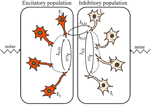
FIGURE 1. A sketch of the noise-perturbed excitatory-inhibitory neural networks. Here, based on the physiological evidences, J_Ej,Ei (resp., J_Ii,Ij and J_Ij,Ii), the weights of the synapses connecting any pair of neurons in the same population J_Ei,Ej and are supposed to be correlated in our model, and J_Ei,Ii and J_Ii,Ei are supposed to be independent.

More precisely, this article is organized as follows. In Section 2, based on Somplinsky’s model of random neural networks, we introduce excitatory and inhibitory populations of intra-correlatively or inter-independently connected neurons, and further include the external perturbations of white noise into the model. Still in this section, we reduce this model of a large-scale into a two-dimensional system using the moment-generating functional and the saddle-point approximation (Eckmann and Ruelle, 1985; Gardiner, 2004; Helias and Dahmen, 2020). In Section 3, along with the reduced system, we study the autocorrelation function, which describes the population-averaged correlation of every state in the two-dimensional system at different time instants, and reveal how the external noise, the coupling strength, and the quantitative proportion of the neurons in two types together affect the autocorrelation function evolving in a long term. Also in this section, we specify some analytical conditions under which the whole system can synchronize as one population in a sense that the autocorrelation functions for the two populations of neurons behave in a consensus manner. Additionally in Section 4, we investigate the maximal Lyapunov exponents for the two populations, respectively, determining whether the system evolves chaotically (Eckmann and Ruelle, 1985), and thus seek numerically out the parameter regions where chaotic dynamics can be suppressed or enhanced. Still in this section, akin to the results obtained in (Schuecker et al., 2018), we numerically detect the parameters’ region where the system evolves in neither linearly stable nor chaotic manner, and also find that the size of such a region crucially depends on the statistical parameters of the two populations of the coupled neurons. We close this article by presenting some discussion and concluding remarks.

2 Model Formulation: Reduction From High-Dimension to Two-Dimension

To begin with, we introduce a neural network model constituting two interacted populations, either of which contains intra- and inter-interacted excitatory or inhibitory neurons. Such a model reads:

$\left\{\begin{array}{c}\hfill \frac{\mathrm{d}{x}_{Ei}}{\mathrm{d}t}=-x_{Ei}+\sum _{j=1}^{N_E}{J}_{Ei,Ej}\varphi \left(x_{Ej}\right)+\sum _{j=1}^{N_I}{J}_{Ei,Ij}\varphi \left(x_{Ij}\right)+\sigma {\xi }_{Ei}\left(t\right),\hfill \\ \hfill \frac{\mathrm{d}{x}_{Ii}}{\mathrm{d}t}=-x_{Ii}+\sum _{j=1}^{N_E}{J}_{Ii,Ej}\varphi \left(x_{Ej}\right)+\sum _{j=1}^{N_I}{J}_{Ii,Ij}\varphi \left(x_{Ij}\right)+\sigma {\xi }_{Ii}\left(t\right),\hfill \end{array}\right.(1)$

where x_Ei and x_Ii represent the states of the excitatory neuron and the inhibitory one, respectively, and ϕ(⋅) stands for the transfer/activation function. Additionally, each J_Ki,Lj is the element of the random connection matrix specified below, and each ξ_Ki(t), as the external perturbation, is supposed to be a white noise with an intensity σ and satisfying

$⟨{\xi }_{Ki}\left(t\right){\xi }_{Lj}\left(s\right)⟩={\delta }_{KL}{\delta }_{ij}\delta \left(t-s\right),$

where K, L ∈ {E, I}, i = 1, 2, … , N_K, j = 1, 2, … , N_L, δ_ij is the Kronecker delta notation, and δ(t − s) is the Dirac delta function with ∫_Rδ(x)f(x)dx = f(0).

On one hand, based on the experimental evidences (Song et al., 2005; Wang et al., 2006; Litwin-Kumar and Doiron, 2012), we suppose that the strength of the intra-coupling between any two of the neurons in the same population is correlated, and further that the mean strength of these couplings does not vanish. Specifically, we suppose the couplings to obey the Gaussian normal distributions as

$\left(\begin{array}{c}\hfill J_{Ei,Ej}\hfill \\ \hfill J_{Ej,Ei}\hfill \end{array}\right)\sim \mathcal{N}\left({\mathit{M}}_E,{\mathit{A}}_E\right),\left(\begin{array}{c}\hfill J_{Ii,Ij}\hfill \\ \hfill J_{Ij,Ii}\hfill \end{array}\right)\sim \mathcal{N}\left({\mathit{M}}_I,{\mathit{A}}_I\right),$

in which

$\begin{array}{ll}\hfill {\mathit{M}}_E& ={\left(\begin{array}{cc}\hfill m_{EE}/N_E\hfill & \hfill m_{EE}/N_E\hfill \end{array}\right)}^{\top },{\mathit{M}}_I={\left(\begin{array}{cc}\hfill m_{II}/N_I\hfill & \hfill m_{II}/N_I\hfill \end{array}\right)}^{\top },\hfill \\ \hfill {\mathit{A}}_E& =g^2\left(\begin{array}{cc}\hfill \frac{1}{N}\hfill & \hfill \frac{{\eta }_E}{N}\hfill \\ \hfill \frac{{\eta }_E}{N}\hfill & \hfill \frac{1}{N}\hfill \end{array}\right),{\mathit{A}}_I=g^2\left(\begin{array}{cc}\hfill \frac{1}{N}\hfill & \hfill \frac{{\eta }_I}{N}\hfill \\ \hfill \frac{{\eta }_I}{N}\hfill & \hfill \frac{1}{N}\hfill \end{array}\right).\hfill \end{array}$

Here, g is the gain parameter modulating the coupling strength of the overall network, each N_E (resp., N_I) stands for the number of neurons in the excitatory (resp., inhibitory) population with N = N_E + N_I, each η_E (resp., η_I) describes the correlation between J_Ei,Ej and J_Ej,Ei (resp., J_Ii,Ij and J_Ij,Ii), two weights of the synapses connecting any pair of the neurons in the same excitatory (resp., inhibitory) population, and m_EE (resp., m_II) characterizes the mean coupling strength among the excitatory (resp., inhibitory) population.

On the other hand, as usual, we assume that the strength of the inter-coupling between any pair of neurons, respectively, from the two populations is independent of the other strength, and further that they obey the following distributions:

$J_{Ei,Ij}\sim \mathcal{N}\left(m_{EI}/N_I,g^2/N\right),J_{Ii,Ej}\sim \mathcal{N}\left(m_{IE}/N_E,g^2/N\right),$

where m_EI (resp., m_IE) is the mean coupling strength from the neurons in the inhibitory (resp., excitatory) population to the ones in the excitatory (resp., inhibitory) population. In the following investigations, we assume that N_E/N_I, the proportion, does not change as N grows. Clearly, there are two kinds of randomnesses simultaneously in this model: J_Ki,Lj, the random coupling strengths, and ξ_Ki, the external perturbations of white noise. In fact, such a model is also suitable for describing coherent or incoherent phenomena that are produced by any system of two populations in addition to the neural populations that are discussed in this article.

Since the coupling matrices used in system (1) are randomly generated during the numerical realizations, simulated dynamics of this system are different almost surely for different selected matrices. To obtain deep, analytical insights to the asymptotic properties of this system as the number of populations N goes to the infinity, we utilize a mean-field technique. Specifically, applying the Martin–Siggia–Rose–de Dominicis–Janssen path integral formula (Martin et al., 1973; De Dominicis, 1976; Janssen, 1976; Chow and Buice, 2015), we transform system (1), stochastic differential equations, into an Itô integral form, and derive the following moment-generating functional:

$Z\left[\mathit{l}\right]\left(\mathit{J}\right)=\int \mathfrak{D}\mathit{x}\int \mathfrak{D}\tilde{\mathit{x}}\exp \left\{S\left[\mathit{x},\tilde{\mathit{x}}\right]-{\tilde{\mathit{x}}}^{\top }\mathit{J}\varphi \left(\mathit{x}\right)+{\mathit{l}}^{\top }\mathit{x}\right\}.(2)$

Here, for ease of reading, we include the tedious calculations for obtaining this functional into Supplementary Appendix SA. The notations in (2) are illustrated as follows:

$S\left[\mathit{x},\tilde{\mathit{x}}\right]={\tilde{\mathit{x}}}^T\left({\partial }_t+1\right)\mathit{x}+\frac{1}{2}{\sigma }^2{\tilde{\mathit{x}}}^{\top }\mathit{x}$

and $\mathit{x}≔{\left(\begin{array}{cc}\hfill {\mathit{x}}_E\hfill & \hfill {\mathit{x}}_I\hfill \end{array}\right)}^{\top }$ represents the trajectories of the neurons with

${\mathit{x}}_E≔{\left(x_{Ei}\left(t\right),t\in \mathbb{R}\right)}_{i=1}^{N_E},{\mathit{x}}_I≔{\left(x_{Ii}\left(t\right),t\in \mathbb{R}\right)}_{i=1}^{N_I}.$

Moreover, after an inverse Fourier transformation of the Dirac delta function, $\tilde{\mathit{x}}≔{\left(\begin{array}{cc}\hfill {\tilde{\mathit{x}}}_E\hfill & \hfill {\tilde{\mathit{x}}}_I\hfill \end{array}\right)}^{\top }$ represents the response field with

${\tilde{\mathit{x}}}_E≔{\left({\tilde{x}}_{Ei}\left(t\right),t\in \mathbb{R}\right)}_{i=1}^{N_E},{\tilde{\mathit{x}}}_I≔{\left({\tilde{x}}_{Ii}\left(t\right),t\in \mathbb{R}\right)}_{i=1}^{N_I},$

and $\mathit{l}≔{\left(\begin{array}{cc}\hfill {\mathit{l}}_E\hfill & \hfill {\mathit{l}}_I\hfill \end{array}\right)}^{\top }$ represents the source field where

${\mathit{l}}_E≔{\left(l_{Ei}\left(t\right),t\in \mathbb{R}\right)}_{i=1}^{N_E},{\mathit{l}}_I≔{\left(l_{Ii}\left(t\right),t\in \mathbb{R}\right)}_{i=1}^{N_I}.$

The formula

${\mathit{l}}^{\top }\mathit{x}≔\sum _{K\in \left\{E,I\right\}}^{}\sum _{i=1}^{N_K}{\int }_R{l}_{K,i}\left(t\right)x_{K,i}\left(t\right)\mathrm{d}t$

denotes the inner product in time and two populations of neurons. In addition, the measure here is denoted formally as

$\int \mathfrak{D}\mathit{x}=\underset{M\to \infty }{\lim }\prod _{K\in \left\{E,I\right\}}^{}\prod _{i=1}^{N_K}\prod _{t=1}^M{\int }_{-\infty }^{+\infty }\mathrm{d}{x}_{Ki}^t$

and

$\int \mathfrak{D}\tilde{\mathit{x}}=\underset{M\to \infty }{\lim }\prod _{K\in \left\{E,I\right\}}^{}\prod _{i=1}^{N_K}\prod _{t=1}^M{\int }_{-i\infty }^{+i\infty }\frac{\mathrm{d}{\tilde{x}}_{Ki}^t}{2\pi \mathrm{i}}.$

Finally, J is an N × N matrix partitioned as

$\mathit{J}=\left(\begin{array}{cc}\hfill {\mathit{J}}_{EE}\hfill & \hfill {\mathit{J}}_{EI}\hfill \\ \hfill {\mathit{J}}_{IE}\hfill & \hfill {\mathit{J}}_{II}\hfill \end{array}\right),$

where ${\mathit{J}}_{KL}={(J_{Ki,Lj})}_{N_K\times N_L}$.

With the moment-generating function Z obtained in (2), we average it over the random coupling matrix J, perform a saddle-point approximation method, and reduce the model into a two-dimensional system, which reads

$\left\{\begin{array}{cc}\frac{\mathrm{d}{x}_E}{\mathrm{d}t}\hfill & =-x_E+{\gamma }_E\left(t\right)+\sigma {\xi }_E\left(t\right)+m_{EE}\langle \varphi \left(x_E\left(t\right)\right)\rangle +m_{EI}\langle \varphi \left(x_I\left(t\right)\right)\rangle ,\hfill \\ \frac{\mathrm{d}{x}_I}{\mathrm{d}t}\hfill & =-x_I+{\gamma }_I\left(t\right)+\sigma {\xi }_I\left(t\right)+m_{IE}\langle \varphi \left(x_E\left(t\right)\right)\rangle +m_{II}\langle \varphi \left(x_I\left(t\right)\right)\rangle .\hfill \end{array}\right.(3)$

Here, for a concise expression, we still include the detailed arguments into Supplementary Appendix SB. The notations used in (3) are defined as follows: ξ_K(t) with K ∈ {E, I} are mutually independent white noises, and γ_K(t) with K ∈ {E, I} are mutually independent stationary Gaussian processes with their means as zeros and their correlations satisfying

$\begin{array}{ccc}\hfill \langle {\gamma }_E\left(t\right){\gamma }_E\left(t^{\prime }\right)\rangle & =\hfill & \frac{g^2}{N}\left[N_E\left(1+{\eta }_E\right)\langle \varphi \left(x_E\left(t\right)\right)\varphi \left(x_E\left(t^{\prime }\right)\right)\rangle +N_I\langle \varphi \left(x_I\left(t\right)\right)\varphi \left(x_I\left(t^{\prime }\right)\right)\rangle \right],\hfill \\ \hfill \langle {\gamma }_I\left(t\right){\gamma }_I\left(t^{\prime }\right)\rangle & =\hfill & \frac{g^2}{N}\left[N_E\langle \varphi \left(x_E\left(t\right)\right)\varphi \left(x_E\left(t^{\prime }\right)\right)\rangle +N_I\left(1+{\eta }_I\right)\langle \varphi \left(x_I\left(t\right)\right)\varphi \left(x_I\left(t^{\prime }\right)\right)\rangle \right].\hfill \end{array}$

3 Dynamics of Autocorrelation Functions

Here, we investigate the dynamics of the autocorrelation functions for the reduced system (3). To this end, letting the left hand side of system (3) equal to zeros yields a stationary solution satisfying

$\left\{\begin{array}{cc}\langle x_E\rangle \hfill & =m_{EE}\langle \varphi \left(x_E\right)\rangle +m_{EI}\langle \varphi \left(x_I\right)\rangle ,\hfill \\ \langle x_I\rangle \hfill & =m_{IE}\langle \varphi \left(x_E\right)\rangle +m_{II}\langle \varphi \left(x_I\right)\rangle .\hfill \end{array}\right.(4)$

For an odd transfer function, we immediately obtain that ⟨x_E⟩ = ⟨x_I⟩ = 0 is a consistent solution. Using the error dynamics as

$\left\{\begin{array}{cc}\delta x_E\left(t\right)\hfill & =x_E\left(t\right)-\langle x_E\rangle ,\hfill \\ \delta x_I\left(t\right)\hfill & =x_I\left(t\right)-\langle x_I\rangle ,\hfill \end{array}\right.$

and assuming these dynamics as stationary Gaussian processes, we define the autocorrelation functions as

$C_E\left(\tau \right)≔\langle \delta x_E\left(t\right)\delta x_E\left(t+\tau \right)\rangle ,C_I\left(\tau \right)≔\langle \delta x_I\left(t\right)\delta x_I\left(t+\tau \right)\rangle ,$

where, physically, these functions represent the population-averaged cross-correlations between the dynamical quantities deviating from the equilibrium states at t and t + τ, two different time instants. For a given difference τ between the time instants, the larger the value of the autocorrelation function, the more correlative manner the deviating dynamics behave in. As will be numerically displayed in the following investigation, with the increase of the difference τ, the value sometimes drops down but sometimes exhibits a non-monotonic tendency.

Further define the variances by c_E0≔C_E(0) and c_I0≔C_I(0), and define c_E∞≔ lim_τ→∞C_E(τ) and c_I∞≔ lim_τ→∞C_I(τ). Through implementing the arguments performed in Supplementary Appendix SC, we get two population-averaged autocorrelation functions obeying the following second-order equations:

$\left\{\begin{array}{cc}\hfill \frac{{\mathrm{d}}^2{C}_E}{\mathrm{d}{\tau }^2}\hfill & \hfill =C_E-\frac{g^2}{N}\left[N_E\left({\eta }_E+1\right)\langle \varphi \left(x_E\left(t\right)\right)\varphi \left(x_E\left(t+\tau \right)\right)\rangle +N_I\langle \varphi \left(x_I\left(t\right)\right)\varphi \left(x_I\left(t+\tau \right)\right)\rangle \right]\hfill \\ \hfill \hfill & \hfill -{\sigma }^2\delta \left(\tau \right),\hfill \\ \hfill \frac{{\mathrm{d}}^2{C}_I}{\mathrm{d}{\tau }^2}\hfill & \hfill =C_I-\frac{g^2}{N}\left[N_E\langle \varphi \left(x_E\left(t\right)\right)\varphi \left(x_E\left(t+\tau \right)\right)\rangle +N_I\left({\eta }_I+1\right)\langle \varphi \left(x_I\left(t\right)\right)\varphi \left(x_I\left(t+\tau \right)\right)\rangle \right]\hfill \\ \hfill \hfill & \hfill -{\sigma }^2\delta \left(\tau \right).\hfill \end{array}\right.(5)$

Notice that each element of system (3) is a Gaussian process and that

$\begin{array}{ll}\hfill ⟨\varphi \left(x_K\left(t\right)\right)\varphi \left(x_K\left(t+\tau \right)\right)⟩& =\frac{1}{2\pi \sqrt{\left|\mathit{A}\right|}}{\iint }_{R^2}\varphi \left(z_1+⟨x_K⟩\right)\varphi \left(z_2+⟨x_K⟩\right)\hfill \\ \hfill & \exp \left(-\frac{1}{2}{\mathit{z}}^T{\mathit{A}}^{-1}\mathit{z}\right)\mathrm{d}{z}_1\mathrm{d}{z}_2,\hfill \end{array}(6)$

where

$\mathit{A}=\left(\begin{array}{cc}\hfill c_{K0}\hfill & \hfill C_K\left(\tau \right)\hfill \\ \hfill C_K\left(\tau \right)\hfill & \hfill c_{K0}\hfill \end{array}\right),K\in \left\{E,I\right\}.$

We thus introduce the notation $f_{\varphi (\cdot +⟨x_K⟩)}(C_K(\tau ),c_{K0})≔⟨\varphi (x_K(t))\varphi (x_K(t+\tau ))⟩$ to represent the function with respect to the autocorrelation and the variance for each K.

In what follows, we analytically and numerically depict how the dynamics of autocorrelation functions are affected by external noise, the coupling strength, and the quantitative proportion of the neurons in two populations. Also we establish conditions under which these two populations of neurons can be synchronized. More precisely, the analytical results are summarized into the following propositions and the numerical results are illustrated after the propositions. The detailed arguments and computations for validating these propositions are included in Supplementary Appendix SD.

Proposition III.1 Define the potentials of the population-averaged motion for the two types of neurons by

$\left\{\begin{array}{cc}{V}_E\left(C_E,C_I;c_{E0},c_{I0}\right)\hfill & =-\frac{1}{2}{C}_E^2+\frac{g^2{N}_E\left(1+{\eta }_E\right)}{N}{f}_{{\rho }_E}\left(C_E,c_{E0}\right)+\frac{g^2{N}_I}{N}{f}_{{\rho }_I}\left(C_I,c_{I0}\right),\hfill \\ V_I\left(C_E,C_I;c_{E0},c_{I0}\right)\hfill & =-\frac{1}{2}{C}_I^2+\frac{g^2{N}_E}{N}{f}_{{\rho }_E}\left(C_E,c_{E0}\right)+\frac{g^2{N}_I\left(1+{\eta }_I\right)}{N}{f}_{{\rho }_I}\left(C_I,c_{I0}\right),\hfill \end{array}\right.(7)$

where

${\rho }_K\left(x\right)={\int }_0^x\varphi \left(y+⟨x_K⟩\right)\mathrm{d}y,K\in \left\{E,I\right\},$

and assume that the external white noise contribute to the initial kinetic energy of all the neurons. Then, the autocorrelation functions satisfy

$\left\{\begin{array}{cc}\frac{1}{2}{C_E^{\prime }}^2+V_E\left(C_E,C_I;c_{E0},c_{I0}\right)\hfill & =\mathrm{c}\mathrm{o}\mathrm{n}\mathrm{s}\mathrm{t},\hfill \\ \frac{1}{2}{C_I^{\prime }}^2+V_I\left(C_E,C_I;c_{E0},c_{I0}\right)\hfill & =\mathrm{c}\mathrm{o}\mathrm{n}\mathrm{s}\mathrm{t},\hfill \end{array}\right.(8)$

and the consistent solutions of c_K∞ and c_K0 satisfy

$\left\{\begin{array}{c}\hfill \frac{{\sigma }^4}{8}+V_E\left(c_{E0},c_{I0};c_{E0},c_{I0}\right)=V_E\left(c_{E\infty },c_{I\infty };c_{E0},c_{I0}\right),\hfill \\ \hfill \frac{{\sigma }^4}{8}+V_I\left(c_{E0},c_{I0};c_{E0},c_{I0}\right)=V_I\left(c_{E\infty },c_{I\infty };c_{E0},c_{I0}\right).\hfill \end{array}\right.(9)$

Additionally, define the powers of the motions (i.e., the derivatives of − V_K as defined above) by

$\left\{\begin{array}{c}\hfill W_E\left(C_E,C_I;c_{E0},c_{I0}\right)=C_E-\frac{g^2{N}_E\left(1+{\eta }_E\right)}{N}{f}_{\varphi \left(\cdot +\langle x_E\rangle \right)}\left(C_E,c_{E0}\right)-\frac{g^2{N}_I}{N}{f}_{\varphi \left(\cdot +\langle x_I\rangle \right)}\left(C_I,c_{I0}\right),\hfill \\ \hfill W_I\left(C_E,C_I;c_{E0},c_{I0}\right)=C_I-\frac{g^2{N}_E}{N}{f}_{\varphi \left(\cdot +\langle x_E\rangle \right)}\left(C_E,c_{E0}\right)-\frac{g^2{N}_I\left(1+{\eta }_I\right)}{N}{f}_{\varphi \left(\cdot +\langle x_I\rangle \right)}\left(C_I,c_{I0}\right),\hfill \end{array}\right.(10)$

and suppose that these powers dissipate in a long timescale, that is,

$W_E\left(c_{E\infty },c_{I\infty };c_{E0},c_{I0}\right)=W_I\left(c_{E\infty },c_{I\infty };c_{E0},c_{I0}\right)=0.(11)$

Then, the two mean states ⟨x_K⟩, the two self-variances c_K0, and the two correlations in a long term c_K∞ for the two populations are analytically existent provided that the equations specified in (4), (9), and (11) are consistent.Particularly, Eq. 8 is actually the energy conservation equation with the potentials V_E,I. Using Eq. 9 yields that the intensity σ of the white noise contributes to the initial kinetic energy $\frac{1}{2}{C_E^{\prime }}^2(0)=\frac{1}{2}{C_I^{\prime }}^2(0)=\frac{{\sigma }^4}{8}$ with the initial velocity $C_E^{\prime }(0)=C_I^{\prime }(0)=\frac{{\sigma }^2}{2}$. Thus, the self-variance c_K0 can admit a higher value than c_K∞.The following proposition further describes the specific forms of the solutions to the consistent equations in 4, 9, 11 under particular conditions.

Proposition III.2 Suppose that all the assumptions set in Proposition III. 1 are all valid. Then, we have the following results.

1) If the transfer function is odd, the two correlations in a long term satisfy c_E∞ = c_I∞ = 0. If σ = 0 is further fulfilled, the two self-variances satisfy c_E0 = c_I0 = 0.

2) If one of the following three conditions is satisfied:

i) all the coupling strengths are independent with each other, i.e., η_E = η_I = 0.

ii) the transfer function is odd and N_Eη_E = N_Iη_I, and.

iii) the mean states satisfy ⟨x_E⟩ = ⟨x_I⟩ and the population sizes with the coupling strengths fulfilling N_Eη_E = N_Iη_I,

then we have C_E(τ) = C_I(τ). This implies that the two populations becomes synchronized in a sense that the two stationary autocorrelation functions behave in the same manner.The following numerical simulations further demonstrate the above analytical findings on the synchronization of the two populations of the neurons. More specifically, for the case where the transfer function is set as an inverse of the tangent function and η_EN_E = η_IN_I, the autocorrelation functions of the two populations are equal all the time according to Proposition III. 2. The fluctuating tendencies of the autocorrelation functions C_E,I(τ) plotted in Figure 2A validate such a case, although this figure presents only one realization for each C_K(τ). Thus, the potentials V_E,I for the two populations are all the same along the time, which implies the occurrence of the synchronized dynamics for the two populations. As seen in Figure 2B (resp., Figure 2C), for the case where η_EN_E = η_IN_I (resp., ⟨x_E⟩ = ⟨x_I⟩) is not satisfied, the dynamics of autocorrelation function for the two populations become different completely. As shown by one realization of each C_K(τ) in Figure 2D, as the coupling correlation coefficient η vanishes, the dynamics behave in a similar manner again. Additionally, as indicated by Proposition III.2, for the transfer function as an inverse of the tangent function, we have c_E∞ = c_I∞ = 0 (see Figures 2A,B); however, for the transfer function as a non-odd function, their autocorrelation functions in a long term may not ever vanish (see Figures 2C,D).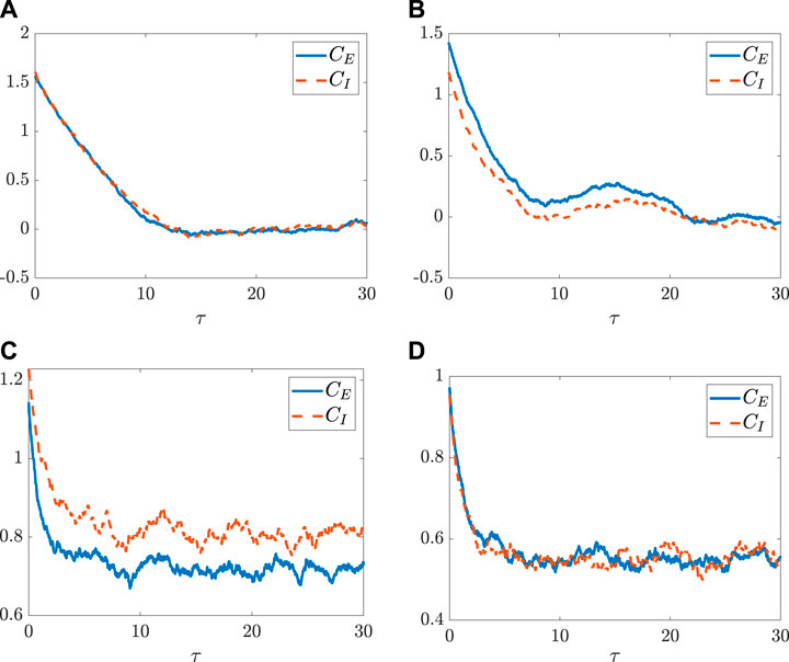

FIGURE 2

FIGURE 2. The autocorrelation functions C_E,I(τ) change with an increase of the time difference τ when the system goes over the time duration from t = 0 to 100. (A) The parameters are set as η_EN_E = η_IN_I = 500 with N_E = 1,500, N_I = 1,000, m_EE = 1, m_IE = 0.75 m_EI = −0.25, m_II = −0.5, g = 1.4, σ = 0.8, ${\eta }_E=\frac{1}{3}$, and ${\eta }_I=\frac{1}{2}$. The transfer function is set as ϕ(x) = arctanx. (B) All the configurations are the same as those set in (A) except for η_I = 0. (C) All the configurations are the same as those set in (A) except for the transfer function set as ϕ(x) = max(arctanx, 0) and the parameters changed as m_IE = 75 and m_II = −50. (D) All the configurations are the same as those set in (C) except for η_E = η_I = 0. Here, only one realization for each functions are numerically presented.

4 Route to Chaos

Since chaos emergent in neural network models is often regarded as a crucial dynamical behavior beneficial to memory storage and association capacity (Lin and Chen, 2009; Haykin et al., 2006; Toyoizumi and Abbott, 2011; Schuecker et al., 2018), it is of great interest to investigate the route of generating chaos in the above system (3) of two populations of neurons. To this end, we calculate the maximal Lyapunov exponent, which quantifies the asymptotic growth rate of the system dynamics for given initial perturbations (Cencini et al., 2010). More precisely, for the two dynamics ${\mathit{x}}_K^1(t)$ and ${\mathit{x}}_K^2(t)$ in one of the populations and with the same realization of the coupling matrix J and the white noise ξ, the maximal Lyapunov exponent (MLE) is defined by

${\lambda }_{\text{max},K}≔\underset{t\to \infty }{\lim }\underset{\Vert {\mathit{x}}_K^1\left(0\right)-{\mathit{x}}_K^2\left(0\right)\Vert \to 0}{\lim }\frac{1}{t}\ln \frac{‖{\mathit{x}}_K^1\left(t\right)-{\mathit{x}}_K^2\left(t\right)‖}{‖{\mathit{x}}_K^1\left(0\right)-{\mathit{x}}_K^2\left(0\right)‖},$

where ‖ ⋅‖ stands for the Euclidean-norm, the number in the superscript corresponds to the different group of the initial values, and the notation (K ∈ {E, I}) in the subscript corresponds to the different population of the neurons. Still for the same realization of the coupling matrix and the white noise, denote, component-wisely, by $x_{Ei}^{\alpha }$ (resp., $x_{Ii}^{\alpha }$) the state of the i-th neuron in the excitatory (resp., inhibitory) population with the α-th group of initial values. Here, α = 1, 2, K ∈ {E, I} and i = 1, 2, … , N_K. Actually, the MLE quantifies how the sensitivity of a system depends on its initial values. We, following the idea presented in Ref. (Derrida and Pomeau, 1986), calculate the MLEs on the two dynamics with only initial values different. Define the distance between these two dynamics, in either population but with different initial values, by

$d_K\left(t\right)≔\frac{1}{N_K}\sum _{i=1}^{N_K}{\left[x_{Ki}^1\left(t\right)-x_{Ki}^2\left(t\right)\right]}^2=\frac{1}{N_K}\sum _{i=1}^{N_K}{\left[\delta x_{Ki}^1\left(t\right)-\delta x_{Ki}^2\left(t\right)\right]}^2,K\in \left\{E,I\right\}.$

Clearly, if λ_max,E > 0 (resp., λ_max,I > 0), that is, the distance between the two dynamics in the excitatory (resp., inhibitory) population grows exponentially with arbitrarily-closed initial values, the dynamics of this population become chaotic. In order to show the conditions under which the chaos occurs, we evaluate d_K(t) as specified above. Thus, direct computation and approximation yield:

$d_K\left(t\right)\approx C_K^{11}\left(t,t\right)+C_K^{22}\left(t,t\right)-C_K^{12}\left(t,t\right)-C_K^{21}\left(t,t\right),$

where

$C_K^{\alpha \beta }\left(s,t\right)≔⟨\delta x_K^{\alpha }\left(s\right)\delta x_K^{\beta }\left(t\right)⟩,K\in \left\{E,I\right\},\alpha ,\beta =\mathrm{1,2}.$

To study the dynamics of d_K(t) more explicitly, we define

$d_K\left(t,t^{\prime }\right)≔C_K^{11}\left(t,t^{\prime }\right)+C_K^{22}\left(t,t^{\prime }\right)-C_K^{12}\left(t,t^{\prime }\right)-C_K^{21}\left(t,t^{\prime }\right),$

where d_K(t, t) = d_K(t), each $C_K^{\alpha \alpha }$ with α = 1, 2 is the autocorrelation function of the dynamics starting from a given group of initial values, and $C_K^{\alpha \beta }$ is the cross-correlation function of the two dynamics with $C_K^{12}=C_K^{21}$. Then, we focus on the collective behaviours of the dynamics starting from different groups of initial values. Particularly, we apply the moment-generating functional, akin to the arguments performed in Supplementary Appendix SA, and obtain

$Z\left[{\mathit{l}}^1,{\mathit{l}}^2\right]\left(\mathit{J}\right)=\prod _{\alpha =1}^2\int \mathfrak{D}{\mathit{x}}^{\alpha }\int \mathfrak{D}{\tilde{\mathit{x}}}^{\alpha }\left(\exp \left\{S\left[{\mathit{x}}^{\alpha },{\tilde{\mathit{x}}}^{\alpha }\right]-{\tilde{\mathit{x}}}^{\alpha \top }\mathit{J}\varphi \left({\mathit{x}}^{\alpha }\right)+{\mathit{l}}^{\alpha \top }{\mathit{x}}^{\alpha }\right\}\right)\exp \left({\sigma }^2{\tilde{\mathit{x}}}^{1\top }{\tilde{\mathit{x}}}^2\right).$

Analogously, averaging it over the random coupling matrix and making a saddle-point approximation (see Supplementary Appendix SE for details) give equivalent dynamical equations as follows.

$\left\{\begin{array}{cc}\frac{\mathrm{d}{x}_E^{\alpha }}{\mathrm{d}t}\hfill & =-x_E^{\alpha }+{\gamma }_E^{\alpha }\left(t\right)+\sigma {\xi }_E^{\alpha }\left(t\right)+m_{EE}\langle \varphi \left(x_E^{\alpha }\left(t\right)\right)\rangle +m_{EI}\langle \varphi \left(x_I^{\alpha }\left(t\right)\right)\rangle ,\hfill \\ \frac{\mathrm{d}{x}_I^{\alpha }}{\mathrm{d}t}\hfill & =-x_I^{\alpha }+{\gamma }_I^{\alpha }\left(t\right)+\sigma {\xi }_I^{\alpha }\left(t\right)+m_{IE}\langle \varphi \left(x_E^{\alpha }\left(t\right)\right)\rangle +m_{II}\langle \varphi \left(x_I^{\alpha }\left(t\right)\right)\rangle ,\hfill \end{array}\right.$

where α = 1, 2, ${\xi }_i^{\alpha }(t)$ is the independent white noise and ${\gamma }_i^{\alpha }(t)$ is the stationary Gaussian process with its mean as zero and its correlation satisfying

$\begin{array}{ccc}\hfill \langle {\gamma }_E^{\alpha }\left(t\right){\gamma }_E^{\beta }\left(t^{\prime }\right)\rangle & =\frac{g^2}{N}\left[N_E\left(1+{\eta }_E\right)\langle \varphi \left(x_E^{\alpha }\left(t\right)\right)\varphi \left(x_E^{\beta }\left(t^{\prime }\right)\right)\rangle +N_I\langle \varphi \left(x_I^{\alpha }\left(t\right)\right)\varphi \left(x_I^{\beta }\left(t^{\prime }\right)\right)\rangle \right],\hfill & \hfill \\ \hfill \langle {\gamma }_I^{\alpha }\left(t\right){\gamma }_I^{\beta }\left(t^{\prime }\right)\rangle & =\frac{g^2}{N}\left[N_E\langle \varphi \left(x_E^{\alpha }\left(t\right)\right)\varphi \left(x_E^{\beta }\left(t^{\prime }\right)\right)\rangle +N_I\left(1+{\eta }_I\right)\langle \varphi \left(x_I^{\alpha }\left(t\right)\right)\varphi \left(x_I^{\beta }\left(t^{\prime }\right)\right)\rangle \right]\hfill & \hfill \end{array}$

with α, β = 1, 2. Now, inspired by the ansatz proposed in (Schuecker et al., 2018), we expand the cross-correlation functions as

$C_K^{12}\left(t,t^{\prime }\right)=C_K\left(t-t^{\prime }\right)+ϵG_K\left(t,t^{\prime }\right),(12)$

where $C_K(t-t^{\prime })=C_K^{11}(t,t^{\prime })=C_K^{22}(t,t^{\prime })$ and K ∈ {E, I}. Hence, we get d_K(t) = −2ϵG_K(t, t) and the dynamical equations for the error dynamics of the cross-correlation functions from the autocorrelation functions as follows:

$\begin{array}{cc}\hfill \left({\partial }_{t^{\prime }}+1\right)\left({\partial }_t+1\right)G_K\left(t,t^{\prime }\right)& =\frac{g^2}{N}\left[N_E\left(1+{\delta }_{KE}{\eta }_E\right)f_{{\varphi }^{\prime }\left(\cdot +\langle x_E\rangle \right)}\left(C_E\left(t-t^{\prime }\right),c_{E0}\right)G_E\left(t,t^{\prime }\right)\right.\hfill \\ \hfill & \left.+N_I\left(1+{\delta }_{KI}{\eta }_I\right)f_{{\varphi }^{\prime }\left(\cdot +\langle x_I\rangle \right)}\left(C_I\left(t-t^{\prime }\right),c_{I0}\right)G_I\left(t,t^{\prime }\right)\right]\hfill \end{array}(13)$

with K ∈ {E, I}. Refer to Supplementary Appendix SF for the detailed arguments on obtaining the above equations. Based on these equations, we can obtain the conditions under which the two populations of the neurons have the same asymptotic behaviours of the MLEs, and specify the critical value of the coupling strength coefficient g where the two populations simultaneously behave in a chaotic manner. We summarize the main conclusion into the following proposition and include the detailed arguments into Supplementary Appendix SG.

Proposition IV.1. Suppose that either one of the conditions assumed in conclusion (2) of Proposition III.2 is satisfied. Then, we have that G_E(t, t′) = G_I(t, t′) and that the MLEs are the same for the two populations. Particularly, g_K,c, the critical value for generating chaos in the two populations, are the same and satisfy

$c_{K0}-g_{K,c}^2\left(1+\frac{N_K{\eta }_K}{N}\right)f_{\varphi }\left(c_{K0},c_{K0}\right)=0,K\in \left\{E,I\right\}.(14)$

We use the numerical simulations to further illustrate the analytical results obtained in Proposition IV. 1. As shown in Figure 3A, when the transfer function is odd and the condition η_EN_E = η_IN_I is satisfied, the MLEs for the two populations are the same. This implies that the sensitivity of two populations depending on the initial values are the same, and also that the critical values for generating chaos in the two populations are the same. However, as shown in Figure 3B, when this condition is not satisfied, the MLEs for the two populations are different, which also indicates that the critical values for chaos emergence are likely different. Particularly, there are some coupling strengths for g (e.g., g = 1.9) such that one population behaves chaotically while the other one does not. This can be illustrated by the chaotic inhibitory population and the non-chaotic excitatory population, which are depicted in Figures 4C,D using the setting g = 1.9. Indeed, as shown in Figure 3C, the MLEs are the same although the transfer function is changed as a non-odd function. The same activation function is used in Figure 2C, where, however, the autocorrelation functions for the two populations are different. This reveals that, for calculating the MLEs, the condition η_EN_E = η_IN_I is probably robust against the selection of the transfer function. In addition, formula (14) is only a sufficient condition for chaos emergence in the two populations that behave in the same manner, and it cannot be expressed in a closed form and hard to be determined, since c_K0 and ⟨x_K⟩ satisfy Eqs 4, 9, 11. It is also worthwhile to mention that the MLEs, shown in Figure 3, for the two populations is not monotonically change with g, which is different from the previous results obtained in (Schuecker et al., 2018). Correspondingly, a more systematic view on how the dynamical behaviors of the two types of neurons change with g are depicted, respectively, in Figure 4.Figures 5, 6 depict how the intensity of white noise σ and the correlation coefficient η_K of the intra-connection influence the MLEs in addition to the coupling strength g. More precisely, as shown in Figure 5, the white noise with the intensity σ can suppress the onset of chaos for both populations of neurons. As for the noise-free case (i.e., σ = 0), the critical values g_K,c for chaos emergence are close to one; however, for the case with noise, g_K,c are larger than 1, which is consistent with the results obtained in (Schuecker et al., 2018). As shown in Figure 6, increasing correlation coefficient η_K of the intra-connection can promote chaos emergence. This is consistent with the findings for the single-population network where increasing the correlation coefficients of the connections yields a broader spectrum distribution of the adjacent matrix along the real axis and leads to chaos emergence (Girko, 1984; Sommers et al., 1988; Rajan and Abbott, 2006). As shown still in Figure 6, enlarging η_K renders the curve of the MLE more monotonously increasing. Additionally, changing η_K in one population can influence dynamics of both populations, but its impacts on the two MLEs are different. In particular, as shown in Figure 7, when η_E is above the value determined by the equation η_EN_E = η_IN_I, it is more likely to enhance the chaos in the population of excitatory neurons.Also, we are to study how the setting in the activation function ϕ affects the phase transition of the studied neuronal networks. To this end, we introduce a parameter a into the transfer function as ϕ_a(x) = arctan(ax). Clearly, the value of a determines the slope of the transfer function at the equilibrium. The larger the slope, the larger the absolute values of the eigenvalues in the vicinity of the equilibrium. As such, increasing the slope likely results in the instability of the neuronal network and promotes the chaos as well. This relation between the slope and the occurrence of chaos is demonstrated in Figure 8, where the numerical simulations on the MLEs and the critical value g_K,c for generating chaos are presented.Finally, the coexistence of linear instability and non-chaos, another interesting phenomenon, was reported for neural models having single population (Schuecker et al., 2018). Here, we validate that such a phenomenon is also present for the above two populations model, but it is crucially related to the selection of several parameters. More precisely, in order to analyze the linear stability of the model, we use its first-order approximation as follows:

$\left\{\begin{array}{c}\hfill \frac{\mathrm{d}{z}_{Ei}}{\mathrm{d}t}=-z_{Ei}+\sum _{j=1}^{N_E}{J}_{Ei,Ej}{\varphi }^{\prime }\left(x_{Ej}\right)z_{Ej}\left(t\right)+\sum _{j=1}^{N_I}{J}_{Ei,Ij}{\varphi }^{\prime }\left(x_{Ij}\right)z_{Ij}\left(t\right),\hfill \\ \hfill \frac{\mathrm{d}{z}_{Ii}}{\mathrm{d}t}=-z_{Ii}+\sum _{j=1}^{N_E}{J}_{Ii,Ej}{\varphi }^{\prime }\left(x_{Ej}\right)z_{Ej}\left(t\right)+\sum _{j=1}^{N_I}{J}_{Ii,Ij}{\varphi }^{\prime }\left(x_{Ij}\right)z_{Ij}\left(t\right),\hfill \end{array}\right.(15)$

where x_Ki is the reference trajectory. The whole network is said to be linearly unstable as ρ is non-negative, where we denote by $\rho ≔\mathrm{m}\mathrm{a}\mathrm{x}\left\{\right.(\mathrm{R}\mathrm{e}(\kappa )|\kappa$ the real part of the eigenvalue of the adjacent matrix specified in $(15)\left.\right\})$. As numerically shown in Figure 9, the whole system is linearly stable until the coupling strength coefficient g goes beyond 1.3. However, as shown in Figure 3B, the populations of the excitatory and the inhibitory neurons display chaotic dynamics, respectively, at the critical points of g = g_E,c = 2 and g = g_I,c = 1.8, which are larger than 1.4. Hence, the phases of neither linear stability nor chaos exist still for the two populations model. Figure 10 shows the dynamical behaviors of the neither linearly stable nor chaotic phase and the linearly stable phase. Particularly, the regions of g for such phases in the respective populations are different: The population of the excitatory neurons having a larger value of the critical point corresponds to a broader range of g.

FIGURE 3

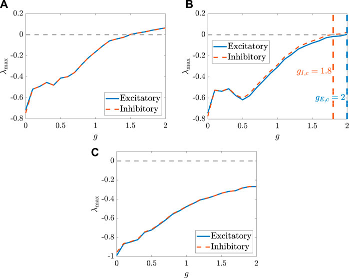
FIGURE 3. The MLEs, respectively, for the two populations, change with the coupling strength coefficient g. (A) The parameters are set as: N_E = 1,500, N_I = 1,000, m_EE = 1, m_IE = 0.75 m_EI = −0.25, m_II = −0.5, σ = 0.8, ${\eta }_E=\frac{1}{3}$, and ${\eta }_I=\frac{1}{2}$. The transfer function is selected as ϕ(x) = arctanx. (B) All the configurations are used in the same manner as those used in (A) except for η_E = −1. (C) All the configurations are used in the same manner as those used in (A) except for the parameters set as m_EI = −25 and m_II = −50 and the transfer function set as ϕ(x) = max(arctanx, 0).

FIGURE 4

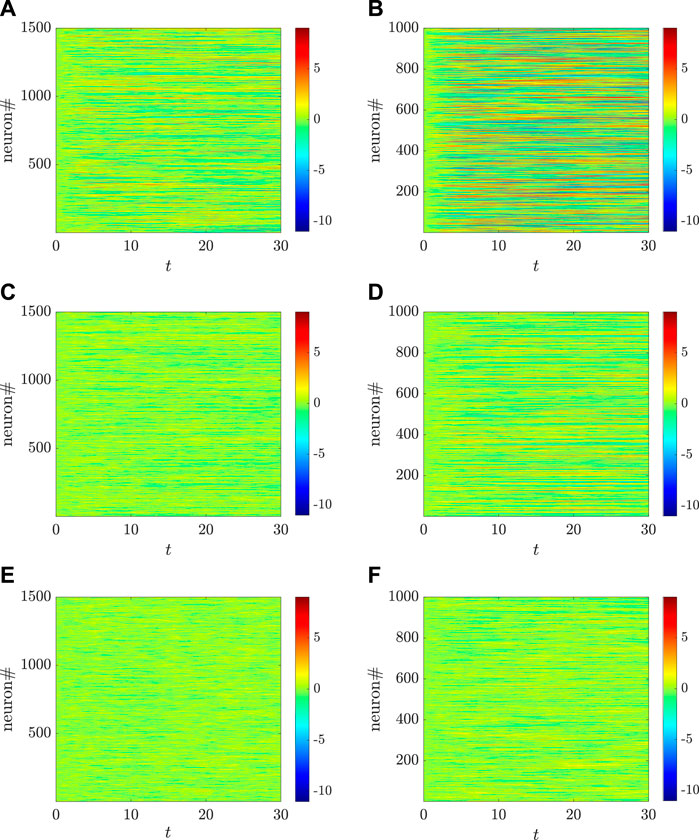
FIGURE 4. Different dynamical behaviors, respectively, for the excitatory (A,C,E) and the inhibitory (B,D,F) populations, change with different coupling strengths for g, where g = 3 [(A,B): both populations are chaotic], g = 1.9 [(C,D): the inhibitory population is chaotic while the excitatory one is non-chaotic], and g = 1.5 [(E,F): both populations are non-chaotic]. Here, the parameters are set as: N_E = 1,500, N_I = 1,000, m_EE = 1, m_IE = 0.75 m_EI = −0.25, m_II = −0.5, σ = 0.8, η_E = −1, and η_I = 0.5. The transfer function is selected as ϕ(x) = arctanx.

FIGURE 5

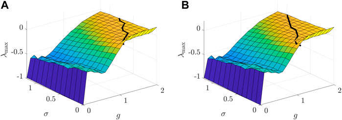
FIGURE 5. The MLEs change with g, the coupling strength coefficient, and σ, the intensity of white noise, respectively, for the population of excitatory neurons (A) and the population of inhibitory neurons (B). The black lines mark g_K,c, the critical points of two populations with given σ. The parameters are set as: N_E = 1,500, N_I = 1,000, m_EE = 1, m_IE = 0.75, m_EI = −0.25, m_II = −0.5, η_E = −1, and η_I = 0.5, and the transfer function is selected as ϕ(x) = arctanx.

FIGURE 6

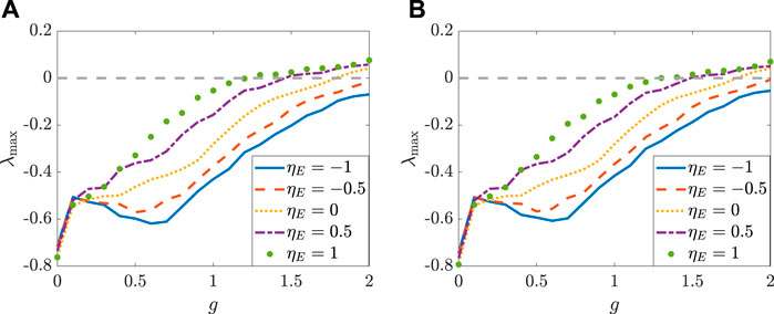
FIGURE 6. The MLEs change with g, the coupling strength coefficient, and η_E, the correlation coefficient of excitatory population, respectively, for the population of the excitatory neurons (A) and the population of the inhibitory neurons (B). The parameters are set as: N_E = 1,500, N_I = 1,000, m_EE = 1, m_IE = 0.75, m_EI = −0.25, m_II = −0.5, σ = 0.8 and η_I = 0, and the transfer function is selected as ϕ(x) = arctanx.

FIGURE 7

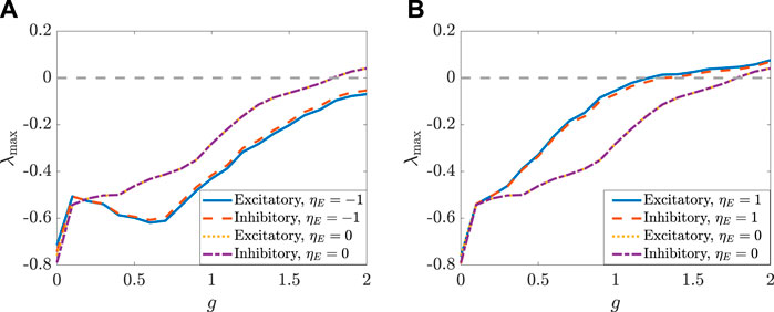
FIGURE 7. The MLEs change with g, the coupling strength coefficient, and η_E, the correlation coefficient of excitatory population, respectively, for the two populations. The parameters are set as: N_E = 1,500, N_I = 1,000, m_EE = 1, m_IE = 0.75 m_EI = −0.25, m_II = −0.5, σ = 0.8 and η_I = 0, and the transfer function is selected as ϕ(x) = arctanx. (A) The comparison between η_E = −1 and η_E = 0. (B)The comparison between η_E = 1 and η_E = 0.

FIGURE 8

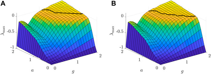
FIGURE 8. The MLEs change simultaneously with g, the coupling strength coefficient, and a, the slope in the transfer function ϕ_a(x) = arctan(ax), respectively, for the population of excitatory neurons (A) and for the population of inhibitory neurons (B). The black curves correspond to g_K,c, the critical values for chaos occurrence in the two populations for different a. Here, the parameters are set as: N_E = 1,500, N_I = 1,000, m_EE = 1, m_IE = 0.75, m_EI = −0.25, m_II = −0.5, η_E = −1, and η_I = 1.

FIGURE 9

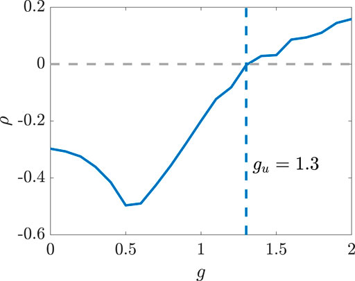
FIGURE 9. The quantity ρ changes with the parameters g and η_E for the two populations model. The parameters are set as: N_E = 1,500, N_I = 1,000, m_EE = 1, m_IE = 0.75, m_EI = −0.25, m_II = −0.5, σ = 0.8, η_E = −1 and η_I = 0.5, and the transfer function is selected as ϕ(x) = arctanx.

FIGURE 10

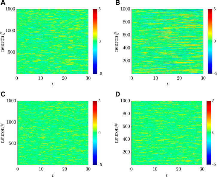
FIGURE 10. Different dynamical behaviors, respectively, for the excitatory (A,C) and the inhibitory (B,D) populations, change with different coupling strengths for g, where g = 1.5 (the first row: the linearly instability phase) and g = 0.8 (the second row: the linearly stable phase). Here, the parameters are set as: N_E = 1,500, N_I = 1,000, m_EE = 1, m_IE = 0.75 m_EI = −0.25, m_II = −0.5, σ = 0.8, η_E = −1, and η_I = 0.5. The transfer function is selected as ϕ(x) = arctanx.

5 Discussion and Concluding Remarks

In this article, inspired by Sompolinsky’s framework on analyzing random neural networks, we have investigated a random neural network model containing both excitatory and inhibitory populations in large scales. We have taken into consideration not only the external perturbations of white noise, but also the randomness of inter- and intra-connections among the neurons. By applying the path integral formalism and the saddle-point approximation, we have reduced the model in large scales into a two-dimensional system with external Gaussian input. Based on the reduced model, we have depicted analytically and numerically how the parameters of populations and randomness influence the synchronization or/and chaotic dynamics of the two populations. Also, we have found different regions of the parameters with which the respective populations have dynamical behaviors of neither linear stability nor chaos.

As for the directions for the further study, we provide the following suggestions. First, although, along with the path integral, the methods used here are applicable to studying population dynamics in neuroscience (Zinn-Justin, 2002; Buice and Cowan, 2007; Chow and Buice, 2015), it is of tremendously tedious calculation to deal with systems having more than two populations. Thus, for multi-population, we suggest to seek additional mean-field methods (Ziegler, 1988; Olivier, 2008; Kadmon and Sompolinsky, 2015) for correspondingly deriving the closed-form equations for autocorrelation functions, obtaining the equivalent stochastic differential equations for the population-averaged Gaussian process, establishing the analytical conditions for synchronization emergence, and finding the phase diagram characterizing the regimes of multi-dynamics.

Second, in light of the spectrum theory of random matrices (Ginibre, 1965; Girko, 1984; Sommers et al., 1988; Tao et al., 2010; Nguyen and O’Rourke, 2014), for single population dynamics with or without external white noise, analytical criteria have been established for stable dynamics (Wainrib and Touboul, 2012) and for chaos emergence (Daniel et al., 2017) as well. In this article, we only use the numerical methods to roughly find the stability regions for the parameters, which suggests that, to obtain more accurate regions, we need to implement the analytical methods using the spectrum theory for random matrices even possessing some particular structures.

Thirdly, we make an assumption that the process is stationary during our analytical investigation and characterize how neurons deviate from their stable states. During the numerical simulations, we treat this assumption through using the data of the processes after a sufficiently long period. As shown in Figure 11, such kind of treatments are reasonable as the processes go eventually stationary. However, the study of the transition to the stationary process or even the non-stationary processes, though rather difficult, could be the potential direction. Indeed, data-driven methods (Hou et al., 2022; Ying et al., 2022) could be the potential tools for studying these transition processes.

FIGURE 11

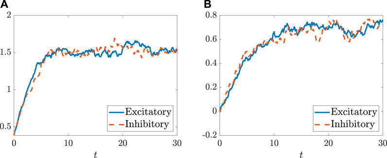
FIGURE 11. The autocorrelation functions ⟨δx_E(t)δx_E(t + τ)⟩ and ⟨δx_I(t)δx_I(t + τ)⟩ change with the evolution of the time t. The parameters are set as η_EN_E = η_IN_I = 500 with N_E = 1,500, N_I = 1,000, m_EE = 1, m_IE = 0.75, m_EI = −0.25, m_II = −0.5, g = 1.4, σ = 0.8, ${\eta }_E=\frac{1}{3}$, and ${\eta }_I=\frac{1}{2}$. The transfer function is set as ϕ(x) = arctanx and the time differences for the two numerical experiments are set as τ = 0 (A) and τ = 5 (B), respectively.

Finally, the coexistence of linearly instability and non-chaos is reported to be beneficial to enhance the information-processing capacity of the model of the single population neural network (Jaeger, 2002; Jaeger and Haas, 2004; Dambre et al., 2012; Schuecker et al., 2018). Here, we also find such a phenomenon in two populations model, and thus suggest to elucidate the relation between this phenomenon and the information-processing capacity in two populations model in the future study.

Data Availability Statement

The original contributions presented in the study are included in the article/Supplementary Material, further inquiries can be directed to the corresponding authors.

Author Contributions

XP and WL conceived the idea, performed the research, and wrote the paper.

Funding

The National Natural Science Foundation of China (Nos 11925103 and 61773125), by the STCSM (Nos 19511132000 and 19511101404), and by the Shanghai Municipal Science and Technology Major Project (No. 2021SHZDZX0103).

Conflict of Interest

The authors declare that the research was conducted in the absence of any commercial or financial relationships that could be construed as a potential conflict of interest.

Publisher’s Note

All claims expressed in this article are solely those of the authors and do not necessarily represent those of their affiliated organizations, or those of the publisher, the editors and the reviewers. Any product that may be evaluated in this article, or claim that may be made by its manufacturer, is not guaranteed or endorsed by the publisher.

Supplementary Material

The Supplementary Material for this article can be found online at: https://www.frontiersin.org/articles/10.3389/fphys.2022.915511/full#supplementary-material

References

Aljadeff J., Stern M., Sharpee T. (2015). Transition to Chaos in Random Networks with Cell-type-specific Connectivity. Phys. Rev. Lett. 114 (8), 088101. doi:10.1103/PhysRevLett.114.088101

PubMed Abstract | CrossRef Full Text | Google Scholar

Boedecker J., Obst O., Lizier J. T., Mayer N. M., Asada M. (2012). Information Processing in Echo State Networks at the Edge of Chaos. Theory Biosci. 131 (3), 205–213. doi:10.1007/s12064-011-0146-8

PubMed Abstract | CrossRef Full Text | Google Scholar

Brunel N. (2000). Dynamics of Sparsely Connected Networks of Excitatory and Inhibitory Spiking Neurons. J. Comput. Neurosci. 8 (3), 183–208. doi:10.1023/a:1008925309027

PubMed Abstract | CrossRef Full Text | Google Scholar

Buice M. A., Cowan J. D. (2007). Field-theoretic Approach to Fluctuation Effects in Neural Networks. Phys. Rev. E Stat. Nonlin Soft Matter Phys. 75 (5), 051919. doi:10.1103/PhysRevE.75.051919

PubMed Abstract | CrossRef Full Text | Google Scholar

Cencini M., Cecconi F., Vulpiani A. (2010). Chaos: From Simple Models to Complex Systems. Singapore: World Scientific.

Google Scholar

Chayes J. T., Chayes L. (1986). Bulk Transport Properties and Exponent Inequalities for Random Resistor and Flow Networks. Commun.Math. Phys. 105 (1), 133–152. doi:10.1007/bf01212346

CrossRef Full Text | Google Scholar

Cheng X., Yuan Y., Wang Y., Wang R. (2020). Neural Antagonistic Mechanism between Default-Mode and Task-Positive Networks. Neurocomputing 417, 74–85. doi:10.1016/j.neucom.2020.07.079

CrossRef Full Text | Google Scholar

Chow C. C., Buice M. A. (2015). Path Integral Methods for Stochastic Differential Equations. J. Math. Neurosc. 5 (1), 8. doi:10.1186/s13408-015-0018-5

PubMed Abstract | CrossRef Full Text | Google Scholar

Dambre J., Verstraeten D., Schrauwen B., Massar S. (2012). Information Processing Capacity of Dynamical Systems. Sci. Rep. 2 (1), 514. doi:10.1038/srep00514

PubMed Abstract | CrossRef Full Text | Google Scholar

Daniel M., Nicolas B., Srdjan O. (2017). Correlations between Synapses in Pairs of Neurons Slow Down Dynamics in Randomly Connected Neural Networks. Phys. Rev. E 97 (6), 062314.

Google Scholar

De Dominicis C. (1976). Techniques de renormalisation de la theorie des champs et dynamique des phenomenes critiques. Le J. de Physique Colloques 37 (C1), 247–253. doi:10.1051/jphyscol:1976138

CrossRef Full Text | Google Scholar

Derrida B., Pomeau Y. (1986). Random Networks of Automata: a Simple Annealed Approximation. Europhys. Lett. 1 (2), 45–49. doi:10.1209/0295-5075/1/2/001

CrossRef Full Text | Google Scholar

Dodds P. S., Harris K. D., Danforth C. M. (2013). Limited Imitation Contagion on Random Networks: Chaos, Universality, and Unpredictability. Phys. Rev. Lett. 110 (15), 158701. doi:10.1103/physrevlett.110.158701

PubMed Abstract | CrossRef Full Text | Google Scholar

Eccles J. C. (1964). The Physiology of Synapses. Berlin: Springer.

Google Scholar

Eckmann J.-P., Ruelle D. (1985). Ergodic Theory of Chaos and Strange Attractors. Rev. Mod. Phys. 57 (3), 617–656. doi:10.1103/revmodphys.57.617

CrossRef Full Text | Google Scholar

Feynman R. P., Lebowitz J. L. (1973). Statistical Mechanics: A Set of Lectures. Phys. Today 26 (10), 51–53. doi:10.1063/1.3128279

CrossRef Full Text | Google Scholar

Forgoston E., Billings L., Schwartz I. B. (2009). Accurate Noise Projection for Reduced Stochastic Epidemic Models. Chaos 19 (4), 043110. doi:10.1063/1.3247350

PubMed Abstract | CrossRef Full Text | Google Scholar

Gardiner C. W. (2004). Handbook of Stochastic Methods: For Physics, Chemistry and the Natural Sciences of Springer Series in Synergetics. third edition, 13. Berlin: Springer-Verlag.

Google Scholar

Gelenbe E. (1993). Learning in the Recurrent Random Neural Network. Neural Comput. 5 (1), 154–164. doi:10.1162/neco.1993.5.1.154

CrossRef Full Text | Google Scholar

Gelenbe E., Yin Y. (2016). “Deep Learning with Random Neural Networks,” in the proceeding of International Joint Conference on Neural Networks, Vancouver. doi:10.1109/ijcnn.2016.7727393

CrossRef Full Text | Google Scholar

Giacomin G., Luçon E., Poquet C. (2014). Coherence Stability and Effect of Random Natural Frequencies in Populations of Coupled Oscillators. J. Dyn. Diff Equat 26 (2), 333–367. doi:10.1007/s10884-014-9370-5

CrossRef Full Text | Google Scholar

Ginibre J. (1965). Statistical Ensembles of Complex, Quaternion, and Real Matrices. J. Math. Phys. 6 (3), 440–449. doi:10.1063/1.1704292

CrossRef Full Text | Google Scholar

Girko V. L. (1984). Circular Law. Theory Probab. Its Appl. 29 (4), 694–706.

Google Scholar

Haykin S., Príncipe J. C., Sejnowski T. J., McWhirter J. (2006). New Directions in Statistical Signal Processing: From Systems to Brains (Neural Information Processing). Cambridge, Massachusetts: The MIT Press.

Google Scholar

Helias M., Dahmen D. (2020). Statistical Field Theory for Neural Networks. Berlin: Springer.

Google Scholar

Hermann G., Touboul J. (2012). Heterogeneous Connections Induce Oscillations in Large-Scale Networks. Phys. Rev. Lett. 109 (1), 018702. doi:10.1103/PhysRevLett.109.018702

PubMed Abstract | CrossRef Full Text | Google Scholar

Horn D., Usher M. (2013). Excitatory–inhibitory Networks with Dynamical Thresholds. Int. J. Neural Syst. 1 (3), 249–257.

Google Scholar

Hou J.-W., Ma H.-F., He D., Sun J., Nie Q., Lin W. (2022). Harvesting Random Embedding For High-Frequency Change-Point Detection in Temporal Complex Systems. Nat. Sci. Rev. 9, nwab228. doi:10.1093/nsr/nwab228

CrossRef Full Text | Google Scholar

Jaeger H., Haas H. (2004). Harnessing Nonlinearity: Predicting Chaotic Systems and Saving Energy in Wireless Communication. Science 304 (5667), 78–80. doi:10.1126/science.1091277

PubMed Abstract | CrossRef Full Text | Google Scholar

Jaeger H. (2002). Short Term Memory in Echo State Networks. GMD-Report 152, GMD - German National Research Institute for Computer Science (2002)

Google Scholar

Janssen H.-K. (1976). On a Lagrangean for Classical Field Dynamics and Renormalization Group Calculations of Dynamical Critical Properties. Z Phys. B 23 (4), 377–380. doi:10.1007/bf01316547

CrossRef Full Text | Google Scholar

Jiang Y., Lin W. (2021). The Role of Random Structures in Tissue Formation: From A Viewpoint of Morphogenesis in Stochastic Systems. Int. J. Bifurcation Chaos 31, 2150171.

CrossRef Full Text | Google Scholar

Kadmon J., Sompolinsky H. (2015). Transition to Chaos in Random Neuronal Networks. Phys. Rev. X 5 (4), 041030. doi:10.1103/physrevx.5.041030

CrossRef Full Text | Google Scholar

Kim S.-Y., Lim W. (2020). Cluster Burst Synchronization in a Scale-free Network of Inhibitory Bursting Neurons. Cogn. Neurodyn 14 (1), 69–94. doi:10.1007/s11571-019-09546-9

PubMed Abstract | CrossRef Full Text | Google Scholar

Landau L. D., Lifshits E. M. (1958). Quantum Mechanics, Non-relativistic Theory. London: Pergamon Press.

Google Scholar

Leng S., Aihara K. (2020). Common Stochastic Inputs Induce Neuronal Transient Synchronization with Partial Reset. Neural Networks 128, 13–21.

PubMed Abstract | CrossRef Full Text | Google Scholar

Li X., Luo S., Xue F. (2020). Effects of Synaptic Integration on the Dynamics and Computational Performance of Spiking Neural Network. Cogn. Neurodyn 14 (4), 347–357. doi:10.1007/s11571-020-09572-y

PubMed Abstract | CrossRef Full Text | Google Scholar

Lin W., Chen G. (2009). Large Memory Capacity in Chaotic Artificial Neural Networks: A View of the Anti-Integrable Limit. IEEE Trans. Neural Networks 20, 1340.

PubMed Abstract | CrossRef Full Text | Google Scholar

Litwin-Kumar A., Doiron B. (2012). Slow Dynamics and High Variability in Balanced Cortical Networks with Clustered Connections. Nat. Neurosci. 15 (11), 1498–1505. doi:10.1038/nn.3220

PubMed Abstract | CrossRef Full Text | Google Scholar

Martin P. C., Siggia E. D., Rose H. A. (1973). Statistical Dynamics of Classical Systems. Phys. Rev. A 8 (1), 423–437. doi:10.1103/physreva.8.423

CrossRef Full Text | Google Scholar

Mastrogiuseppe F., Ostojic S. (2017). Intrinsically-generated Fluctuating Activity in Excitatory-Inhibitory Networks. PLoS Comput. Biol. 13 (4), e1005498. doi:10.1371/journal.pcbi.1005498

PubMed Abstract | CrossRef Full Text | Google Scholar

Mur-Petit J., Polls A., Mazzanti F. (2002). The Variational Principle and Simple Properties of the Ground-State Wave Function. Am. J. Phys. 70 (8), 808–810. doi:10.1119/1.1479742

CrossRef Full Text | Google Scholar

Nguyen H. H., O’Rourke S. (2014). The Elliptic Law. Int. Math. Res. Not. 2015 (17), 7620–7689. doi:10.1093/imrn/rnu174

CrossRef Full Text | Google Scholar

Olivier F. (2008). A Constructive Mean Field Analysis of Multi Population Neural Networks with Random Synaptic Weights and Stochastic Inputs. Front. Comput. Neurosci. 3 (1), 1.

Google Scholar

Omri H., David H., Olaf S. (2015). Asynchronous Rate Chaos in Spiking Neuronal Circuits. PloS Comput. Biol. 11 (7), e1004266.

PubMed Abstract | Google Scholar

Parshani R., Carmi S., Havlin S. (2010). Epidemic Threshold for the Susceptible-Infectious-Susceptible Model on Random Networks. Phys. Rev. Lett. 104 (25), 258701. doi:10.1103/physrevlett.104.258701

PubMed Abstract | CrossRef Full Text | Google Scholar

Pontes-Filho S., Lind P., Yazidi A., Zhang J., Hammer H., Mello G. B. M., et al. (2020). A Neuro-Inspired General Framework for the Evolution of Stochastic Dynamical Systems: Cellular Automata, Random Boolean Networks and Echo State Networks towards Criticality. Cogn. Neurodyn 14 (5), 657–674. doi:10.1007/s11571-020-09600-x

PubMed Abstract | CrossRef Full Text | Google Scholar

Price R. (1958). A Useful Theorem for Nonlinear Devices Having Gaussian Inputs. IEEE Trans. Inf. Theory 4 (2), 69–72. doi:10.1109/tit.1958.1057444

CrossRef Full Text | Google Scholar

Rajan K., Abbott L. F., Sompolinsky H. (2010). Stimulus-dependent Suppression of Chaos in Recurrent Neural Networks. Phys. Rev. E Stat. Nonlin Soft Matter Phys. 82 (1), 011903. doi:10.1103/PhysRevE.82.011903

PubMed Abstract | CrossRef Full Text | Google Scholar

Rajan K., Abbott L. F. (2006). Eigenvalue Spectra of Random Matrices for Neural Networks. Phys. Rev. Lett. 97 (18), 188104. doi:10.1103/physrevlett.97.188104

PubMed Abstract | CrossRef Full Text | Google Scholar

Schuecker J., Goedeke S., Helias M. (2018). Optimal Sequence Memory in Driven Random Networks. Phys. Rev. X 8 (4), 041029. doi:10.1103/physrevx.8.041029

CrossRef Full Text | Google Scholar

Shen Y., Wang J. (2012). Robustness Analysis of Global Exponential Stability of Recurrent Neural Networks in the Presence of Time Delays and Random Disturbances. IEEE Trans. Neural Netw. Learn. Syst. 23 (1), 87–96. doi:10.1109/tnnls.2011.2178326

PubMed Abstract | CrossRef Full Text | Google Scholar

Sommers H. J., Crisanti A., Sompolinsky H., Stein Y. (1988). Spectrum of Large Random Asymmetric Matrices. Phys. Rev. Lett. 60 (19), 1895–1898. doi:10.1103/physrevlett.60.1895

PubMed Abstract | CrossRef Full Text | Google Scholar

Sompolinsky H., Crisanti A., Sommers H. J. (1988). Chaos in Random Neural Networks. Phys. Rev. Lett. 61 (3), 259–262. doi:10.1103/physrevlett.61.259

PubMed Abstract | CrossRef Full Text | Google Scholar

Song S., Sjöström P. J., Reigl M., Nelson S., Chklovskii D. B. (2005). Highly Nonrandom Features of Synaptic Connectivity in Local Cortical Circuits. PLoS Biol. 3 (3), e68. doi:10.1371/journal.pbio.0030068

PubMed Abstract | CrossRef Full Text | Google Scholar

Tao T., Vu V., Krishnapur M. (2010). Random Matrices: Universality of ESDs and the Circular Law. Ann. Probab. 38 (5), 2023–2065. doi:10.1214/10-aop534

PubMed Abstract | CrossRef Full Text | Google Scholar

Teng D., Song X., Gong G., Zhou J. (2018). Learning Robust Features by Extended Generative Stochastic Networks. Int. J. Model. Simul. Sci. Comput. 9 (1), 1850004. doi:10.1142/s1793962318500046

CrossRef Full Text | Google Scholar

Toyoizumi T., Abbott L. F. (2011). Beyond the Edge of Chaos: Amplification and Temporal Integration by Recurrent Networks in the Chaotic Regime. Phys. Rev. E Stat. Nonlin Soft Matter Phys. 84 (5), 051908. doi:10.1103/PhysRevE.84.051908

PubMed Abstract | CrossRef Full Text | Google Scholar

Transience N. B. (2002). Recurrence and Critical Behavior for Long-Range Percolation. Commun. Math. Phys. 226 (3), 531–558.

Google Scholar

van Vreeswijk C., Sompolinsky H. (1996). Chaos in Neuronal Networks with Balanced Excitatory and Inhibitory Activity. Science 274 (5293), 1724–1726. doi:10.1126/science.274.5293.1724

PubMed Abstract | CrossRef Full Text | Google Scholar

Wainrib G., Gilles , Touboul J., Jonathan (2012). Topological and Dynamical Complexity of Random Neural Networks. Phys. Rev. Lett. 110 (11), 118101. doi:10.1103/PhysRevLett.110.118101

PubMed Abstract | CrossRef Full Text | Google Scholar

Wang X. R., Lizier J. T., Prokopenko M. (2014). Fisher Information at the Edge of Chaos in Random Boolean Networks. Artif. Life 17 (4), 315–329. doi:10.1162/artl_a_00041

CrossRef Full Text | Google Scholar

Wang Y., Markram H., Goodman P. H., Berger T. K., Ma J., Goldman-Rakic P. S. (2006). Heterogeneity in the Pyramidal Network of the Medial Prefrontal Cortex. Nat. Neurosci. 9 (4), 534–542. doi:10.1038/nn1670

PubMed Abstract | CrossRef Full Text | Google Scholar

Wang Z., Wang R. (2014). Energy Distribution Property and Energy Coding of a Structural Neural Network. Front. Comput. Neurosci. 8 (14), 14. doi:10.3389/fncom.2014.00014

PubMed Abstract | CrossRef Full Text | Google Scholar

Wang Z., Wang R., Fang R. (2015). Energy Coding in Neural Network with Inhibitory Neurons. Cogn. Neurodyn 9 (2), 129–144. doi:10.1007/s11571-014-9311-3

PubMed Abstract | CrossRef Full Text | Google Scholar

Yang Y., Xiang C., Dai X., Zhang X., Qi L., Zhu B., et al. (2022). Chimera States and Cluster Solutions in Hindmarsh-Rose Neural Networks with State Resetting Process. Cogn. Neurodyn 16 (1), 215–228. doi:10.1007/s11571-021-09691-0

PubMed Abstract | CrossRef Full Text | Google Scholar

Ying X., Leng S.-Y., Ma H.-F., Nie Q., Lin W. (2022). Continuity Scaling: A Rigorous Framework for Detecting and Quantifying Causality Accurately. Research 2022, 9870149. doi:10.34133/2022/9870149

PubMed Abstract | CrossRef Full Text | Google Scholar

Yuan Y., Pan X., Wang R. (2021). Biophysical Mechanism of the Interaction between Default Mode Network and Working Memory Network. Cogn. Neurodyn 15 (6), 1101–1124. doi:10.1007/s11571-021-09674-1

PubMed Abstract | CrossRef Full Text | Google Scholar

Zhu Q., Ma H., Lin W. (2019). Detecting Unstable Periodic Orbits Based Only on Time Series: When Adaptive Delayed Feedback Control Meets Reservoir Computing. Chaos 29, 093125.

PubMed Abstract | CrossRef Full Text | Google Scholar

Zhou S., Guo Y., Liu M., Lai Y.-C., Lin W. (2019). Random Temporal Connections Promote Network Synchronization. Phys. Rev. E 100, 032302.

PubMed Abstract | CrossRef Full Text | Google Scholar

Ziegler K. (1988). On the Mean Field Instability of a Random Model for Disordered Superconductors. Commun.Math. Phys. 120 (2), 177–193. doi:10.1007/bf01217961

CrossRef Full Text | Google Scholar

Zinn-Justin J. (2002). Quantum Field Theory and Critical Phenomena. Oxford: Clarendon Press.

Google Scholar