
94% of researchers rate our articles as excellent or good
Learn more about the work of our research integrity team to safeguard the quality of each article we publish.
Find out more
ORIGINAL RESEARCH article
Front. Physiol., 14 October 2021
Sec. Computational Physiology and Medicine
Volume 12 - 2021 | https://doi.org/10.3389/fphys.2021.733449
This article is part of the Research TopicArtificial Intelligence in Human PhysiologyView all 9 articles
 Miguel Ángel Cámara-Vázquez1
 Ismael Hernández-Romero1
 Eduardo Morgado-Reyes1
 Maria S. Guillem2
 Andreu M. Climent2*†
 Oscar Barquero-Pérez1,2*†
Atrial fibrillation (AF) is characterized by complex and irregular propagation patterns, and AF onset locations and drivers responsible for its perpetuation are the main targets for ablation procedures. ECG imaging (ECGI) has been demonstrated as a promising tool to identify AF drivers and guide ablation procedures, being able to reconstruct the electrophysiological activity on the heart surface by using a non-invasive recording of body surface potentials (BSP). However, the inverse problem of ECGI is ill-posed, and it requires accurate mathematical modeling of both atria and torso, mainly from CT or MR images. Several deep learning-based methods have been proposed to detect AF, but most of the AF-based studies do not include the estimation of ablation targets. In this study, we propose to model the location of AF drivers from BSP as a supervised classification problem using convolutional neural networks (CNN). Accuracy in the test set ranged between 0.75 (SNR = 5 dB) and 0.93 (SNR = 20 dB upward) when assuming time independence, but it worsened to 0.52 or lower when dividing AF models into blocks. Therefore, CNN could be a robust method that could help to non-invasively identify target regions for ablation in AF by using body surface potential mapping, avoiding the use of ECGI.
Atrial fibrillation (AF) is the most common type of arrhythmia in clinical practice, affecting more than 33 million patients in the world (Chugh et al., 2014). AF is also a condition that increases the risk of the patients to suffer embolism, cardiac failure, stroke, and in the worst of cases, death (Fuster et al., 2006).
Therefore, one of the clinical goals in AF patients is to restore sinus rhythm. This objective can be achieved by pharmacological treatment (Lip and Tse, 2007), but termination of arrhythmic processes is usually accomplished by ablation of the cardiac tissue. Main targets of ablation are AF onset locations and drivers responsible for AF perpetuation (Guillem et al., 2016).
Previous human in vivo research showed different strategies to locate AF drivers and guide pulmonary veins isolation (PVI). In the case of invasive mapping procedures (Narayan et al., 2012; Krummen et al., 2017; Navara et al., 2018), several catheters are introduced inside the atrial chambers to record from 8 to 128 simultaneous electrograms (EGM) (Narayan et al., 2012). Despite the number of intracardiac signals, the large distance between catheter sensors (up to 1–2 cm) and the complex atrial anatomy limits the capability of intracardiac mapping systems to characterize the global electrical activity in AF (Oesterlein et al., 2016). Non-invasive procedures based on ECG imaging (ECGI) have been also tested to guide PVI (Haissaguerre et al., 2013, 2014; Dubois et al., 2015). However, PVI success rate gets lower in persistent AF, and phase singularity (PS)-guided ablation is suggested to be a reliable alternative for these more complicated cases (De Greef et al., 2018; Rottner et al., 2020).
Although ECGI has not been validated during AF propagation patterns, it has been demonstrated as a promising tool to identify AF drivers and guide ablation procedures (Cuculich et al., 2010; Haissaguerre et al., 2013, 2014; Pedrón-Torrecilla et al., 2016; Rodrigo et al., 2016). ECGI combines both numerical modeling of the bioelectric properties of the thorax and signal processing, with the aim of reconstructing the electrophysiological activity on the heart surface by using a non-invasive recording of body surface potentials (BSP) (Brooks and Macleod, 1997; Gulrajani, 1998). However, the inverse problem of ECGI has several drawbacks. First, it requires an accurate mathematical modeling of both atria and torso, mainly from CT or MR images. Next, the inverse problem of ECGI is ill-posed because the propagation between the epicardium and the torso implies information loss due to signal attenuation (Rodrigo et al., 2014), and BSP are also blurred compared to the signals on the heart due to the laws of electromagnetic field theory. Therefore, regularization methods are needed to obtain reliable and stable epicardial potential reconstructions (Tikhonov and Arsenin, 1977; Oster and Rudy, 1992; MacLeod and Brooks, 1998; Pedron-Torrecilla et al., 2011; Milanic et al., 2014). For these reasons, inverse problem-based approaches still need further improvement.
In the last decade, machine learning (ML) and deep learning (DL) techniques have undergone considerable development in bioengineering, and this include novel research in AF. For example, DL has been used in AF detection by using recurrent neural networks (RNN) and convolutional neural networks (CNN) (Xiong et al., 2017), by STFT, stationary wavelet transform and CNN (Xia et al., 2018), and in the detection of individuals at risk of suffering from Paroxysmal AF by CNN (Pourbabaee et al., 2018). However, most of AF-based studies do not include the estimation of ablation targets. Nonetheless, recent research showed that ML and DL methods can be also used in more complex tasks, like heart surface potentials estimation from BSP using autoencoders (Bujnarowski et al., 2020) and rotor identification from 12-lead ECG using decision trees (Luongo et al., 2021).
Therefore, in this study we propose to model the location of AF drivers from BSP as a supervised classification problem. We used CNN, which accounts for spatial characteristics, to address the location of AF drivers from previously labeled realistic computerized AF models (Figuera et al., 2016; Cámara-Vázquez et al., 2020).
The remaining of the study is organized as follows. In Section 2, we introduce the computational models used for this study, the experimental set-up, performance metrics, and DL architecture. Final results are summarized in sections 3 and in section 4 main conclusions are presented.
Geometric Models and EGM Computation
Realistic 3D model for the atrial anatomy was composed of 284,578 nodes and 1,353,783 tetrahedrons (673.4 ± 130.3μm between nodes) (Dössel et al., 2012) that considers a simplified single endocardium-epicardium layer for the atrial tissue.
We simulated 13 different AF propagation patterns in both left atria (LA) and right atria (RA), with different complexity and driver positions: posterior left atrial wall (PLAW), left inferior pulmonary vein (LIPV), left superior pulmonary vein (LSPV), right inferior pulmonary vein (RIPV), right superior pulmonary vein (RSPV), right atrial appendage (RAA), and right atria free wall (RAFW). Sampling rate of the signals was fs = 500Hz, while their duration ranged from 2 to 5 s.
The final computerized models were comprised of N = 2, 048 nodes for atria, and M between 2,206 and 3,970 nodes for torsos (10 different geometries were used), under the assumption of a homogeneous, unbounded, and quasi-static conducting medium by summing up all effective dipole contributions over the entire model (García-Molla et al., 2014; Figuera et al., 2016; Pedrón-Torrecilla et al., 2016; Rodrigo et al., 2017). Therefore, the EGMs of the entire model were computed as:
where is the EGM signal at the measuring point, Vm is the transmembrane potential distribution across the atria, is the distance vector between the measuring point and a point in the tissue domain, and r is its corresponding scalar distance. The transmembrane potentials were defined in a scattered 3D mesh, so the gradient was computed by interpolating a quadratic function that involves two surrounding points (Lawson, 1984):
where Vm,i and Vm,j are the transmembrane potentials at the points i and j; x, y, z are the incremental Cartesian coordinates from j to i, and coefficients c1 to c9 were computed by the least square method in, at least, nine neighboring points of each location.
Atrial cell model
The atrial cell model used is based on the one proposed in Nygren et al. (1998) and Koivumäki et al. (2014), where the electrical activity of a single myocyte is described in terms of their transmembrane potentials and ionic currents:
where V is the transmembrane potential, Iion is the transmembrane ionic currents, and Cm is the cell membrane capacitance.
Then, the electrical propagation across the atrial tissue was simulated by including the transmembrane currents caused by the intercellular Gap junction current (due to the transmembrane potential gradient) in the previous formulation:
where Vk is the transmembrane potential at node k, Vi is the transmembrane potential at the neighbor node i, Dk,i is the diffusion coefficient between the node k and i, and dk,i is the distance between those nodes. Since the atrial electrical conduction is anisotropic (its velocity is higher in the longitudinal fiber orientation than at transverse), the diffusion coefficient Dk,i that modulates the intercellular ionic current is determined as follows:
where α is the angle between the longitudinal fiber orientation and the vector linking nodes k and i, and Dlong and Dtrans are the longitudinal and transverse diffusion coefficients, respectively (Rodrigo, 2016). Fibrotic and scar tissues were modeled by setting the diffusion values of the involved nodes to 0. In the case of the fibrotic tissue, a certain percentage of random nodes were disconnected, depending on the pattern to simulate. The final system of differential equations was solved by Runge-Kutta integration (using NVIDIA Tesla C2075 6G).
We proposed to address the location of AF drivers as a supervised classification problem. We divided the atria into seven regions (Figure 1, right) where the AF driver can be found (Haissaguerre et al., 2014). Each region, which ranged from 1 to 7, represents a class to which the AF driver belongs. To obtain labeled data, AF driver location from the computerized model was manually classified into one region for each time-instant. An additional label (0) is assigned when no driver is found.
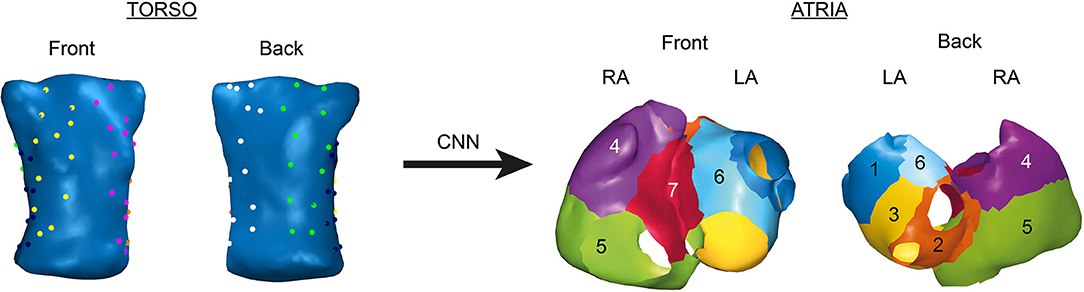
Figure 1. Position of the electrodes for body surface potential mapping (BSPM, left) and regions in atria where AF drivers can be found (right).
Input data for DL algorithms are simulated BSP from each of the 10 torso geometries available. To compute the initial BSP y, the forward problem of ECGI was solved by computing the corresponding M × N transfer matrix A using the boundary element method (Barr et al., 1977; De Munck, 1992; Pedrón-Torrecilla et al., 2016):
where yt are the BSP from each time instants. Those simulated BSP must be referenced to the Wilson Central Terminal (WCT). This step is essential since real ECG recordings are referenced to this point due to the electrical noise of the ground, and it can be mathematically represented as:
where ECGnotref is the not-corrected ECG, ECGWCT is the WCT signal, computed as the average of the ECG signals at the WCT points, and ECG is the final corrected ECG. Therefore, if we apply the same methodology to BSP, yt referenced signals can be computed as:
where NWCT is the number of WCT points, and MWCT is a matrix of zeros except the rows that correspond to the WCT leads, that have the same values as the corresponding rows of the A matrix (Rodrigo, 2016). Therefore, to directly compute the BSP referenced to the WCT, it is possible to compute a corrected ACTW matrix as:
Once the WCT-referenced simulated BSP were computed, they were corrupted with additive Gaussian noise and filtered using: fourth-order bandpass Butterworth filter (fc1 = 3 Hz and fc2 = 30 Hz) (Figuera et al., 2016; Pedrón-Torrecilla et al., 2016). Signal-to-noise ratios (SNR) ranged from 5 to 50 dB. Finally, a set of 64 electrodes from each torso were chosen to represent a realistic multi-electrode vest used in electrophysiological studies, as shown in Figure 1 (left).
To obtain final input data, we represented the layout of electrodes in Figure 1 as images. For this purpose, we build two different types of tensors for each time instant (see Figure 2):
• 3-channel tensor. This first approach consists on creating 3D matrices of shape (6 × 4 × 3). The first and last channel contain the BSP of the torso and back, respectively (24 electrodes each), whereas the second channel contains BSP from the sides (16 electrodes distributed on the last 4 rows, while the rest are filled with zeroes).
• 1-channel tensor. This second approach consists on organizing the BSP in a single-channel 2D matrix of shape (6 × 16 × 1). To do that, we considered a multielectrode vest as a cylinder that was unrolled to a 12-column flat layout. Then, we added two additional mirror columns to each side of the matrix to represent the fact that the first and last columns of the tensor are in touch in a real 3D geometry. Finally, since sides electrodes are four for each column (instead of 6), the empty values are filled with the mean of the three nearest electrodes.
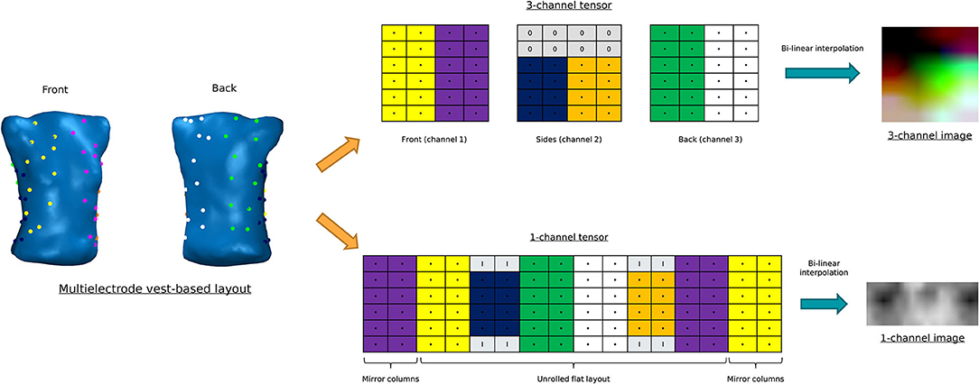
Figure 2. Construction of the different tensor layouts. Above: 3-channel tensor. Below: 1-channel tensor.
Finally, to increase the size of the images, we performed a bilinear interpolation to create tensors with shape (150 × 152 × 3) and (78 × 192 × 1), respectively.
CNN are a type of DL algorithm used mainly in image recognition and image classification. Comparing with other types of DL algorithms, this approach has a superior ability to extract features, increasing classification performance (Krizhevsky et al., 2017).
CNN-based architectures consist on the following layers:
• Input layer. In this case, input data are an image, i.e., a 3D matrix. This input matrix is also named as tensor.
• Convolutional layer. In this type of layer, a filter of size (s, t) is applied to the input tensor. The main aim of the convolutional layer is to extract feature maps that can reflect certain characteristics of interest (edges, shape detection, etc.) (Li et al., 2019). This filtering process is performed using the convolution operation, which can be mathematically represented as:
where ai,j is the output (activation) on coordinates (i,j), xi+m, j+n is the value of the input tensor in coordinates (i+m, j+n), wm,n is the coefficient of the filter in coordinates (m,n), b is the bias, and f(·) is a nonlinear activation function.
• Pooling layer. This type of layers is frequently used between convolutional layers, since they reduce the amount of information that convolutional layers generate. There are several ways to implement a pooling layer, and one of the most used is the max-pooling. In this case, a non-overlapped window is applied to the input feature map, and the output is the maximum value of the considered window. If we consider a square window, the output feature map shape will be reduced in a 1/m factor, where m is the dimension of the window.
• Dense layer. After applying a certain combination of convolutional and pooling layers, a multilayer perceptron (MLP) can be applied afterwards. Therefore, it is necessary to create an unidimensional vector from the output of the convolutional network (flatten operation). As explained before, the output layer of the MLP will have one unit for each value the network should output.
The proposed CNN-based architecture is shown in Figure 3A. Input data are tensors of shape (150 × 152 × 3) or (78 × 192 × 1), depending on the tensor architecture evaluated. We used three convolutional layers with 32, 64 and 64 filters with (3 × 3) size. ReLU activation function was used in both convolutional layers. Max-pooling is applied after each convolutional layer [(2,2) window size]. Final dense layers are composed by layers of (128, 64) units (ReLU activation function), while the output layer is a Softmax layer composed by 8 units, one for each label. Finally, we used dropout between dense layers (0.6 dropout rate) to avoid overfitting.
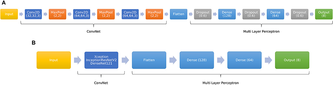
Figure 3. Schematic overview of the CNN-based proposed architectures. (A) Custom CNN. (B) Adaptation of pre-trained network to a 8-unit output.
Finding the right parameters for a CNN (number and dimensions of layers, pooling, etc.) can be a very complicated task, and training this type of network is also very computationally expensive. To address this task, there are several models that were previously trained with a certain dataset that can be also used to solve similar problems. This approach is called transfer learning (Pan and Yang, 2009).
In this study, we decided to adapt the DenseNet121 (DN121, Huang et al., 2016), InceptionResNetV2 (IRNV2, Szegedy et al., 2016), and Xception (Chollet, 2016) models to our problem. These models were trained with the ImageNet database (Russakovsky et al., 2015), comprised of 14 million images corresponding to 1,000 different classes. Therefore, since we want to obtain an output with the prediction for 8 cases instead of 1,000, we added several fully connected layers to the output of the pre-trained models. This adaptation is showed in Figure 3B. Dense layers were composed of (128,64) units (ReLU activation function), while the output layer is a Softmax layer composed by 8 units.
Finally, it is essential to remark that these pre-trained models require 3-channel input tensors. Therefore, to use the previously described 1-channel tensor, we decided to repeat the 2D matrix twice to obtain a 3-channel tensor [(78 × 192 × 3) shape].
To assess the performance of the implemented DL models, we used four different metrics:
• Accuracy (Acc). It is measured as
where TPfull is the total number of well-classified drivers (true positives), and Total is the total number of drivers.
• Cohen's Kappa (κ). It is a robust statistic used for rating reliability testing (McHugh, 2012), and is computed as
where po is the relative agreement among raters (identical to accuracy), and pe the hypothetical probability of chance agreement. A score of 1 represents a perfect agreement between raters, and a score of 0 represents the agreement that can be expected from random chance. Scores less than 0 mean that there is less agreement than chance.
• Sensitivity (or true positive rate, TPR). It is the proportion of positive samples for a class that are correctly classified. It is measured as:
where TP is the number of well-classified drivers for a certain class (true positives), and FN is the number of drivers that was wrongly classified to another class (false negatives). It is considered a measure of how well a test can identify true positives.
• Specificity (or true negative rate, TNR). It is the proportion of negative samples for a class that are correctly classified. It is measured as:
where TN is the number of drivers that did not belong to a certain class that were correctly classified (true negatives), and FP is the number of drivers that was classified as positive for the same class, but they correspond to another class (false positives). It is considered a measure of how well a test can identify true negatives.
Final data set is composed of input data tensors, xi, of shape (150 × 152 × 3) or (78 × 192 × 1) [(78 × 192 × 3) in the case of the pre-trained models], obtained from 64 BSP electrodes, and their corresponding label yi, which can have values 0, 1, …, 7.
Training and test sets were split using two different approaches:
• Time independence of input data. In this case, each time instant is considered as an independent sample. The whole data set was then randomly split into training (80%) and test (20%) sets, using hold-out validation during the training process (20%). In this scenario, samples from each AF model are randomly distributed to the training, validation, and test sets, but training, validation, and test processes are carried out with completely different samples, i.e., samples from the training set are not used in the validation and test sets.
• Division of AF models in consecutive blocks. To describe a more realistic scenario, we divided each AF computerized model in three independent blocks: training (first 80% of the length of the signals), hold-out validation (last 20% of the training set), and test (final 20% of the length of the signals). Therefore, these three blocks contain consecutive samples, i.e., the training process is carried out using the first block of time instants, and test is achieved with the last block of samples.
On the other hand, we had to address imbalance of data. In our computerized models, there are several atrial areas where the driver only appears in one single AF computerized model, whereas other areas are more susceptible of containing a driver. Therefore, there are several atria regions that are over represented in the data set. To address this problem, we tried to weigh the classes accordingly to the probability of occurrence (class weight). It applies a higher penalization in wrong classifications in under-represented classes.
Regarding the training process, we trained the different models for a maximum number of epochs of 1,000, with reduction in the learning rate and early stopping if there is no improvement in the loss value during a certain number of training epochs. Moreover, we use the model checkpoint technique to get the best model obtained during the training process according to a metric of interest (loss value for the custom CNN, and validation loss for the pre-trained CNN). Finally, in the case of the pre-trained models, we followed two different training approaches: training the dense layers and the last two convolutional layers (while freezing the rest of the CNN, partial training), and re-training the whole pre-trained network (full training).
The first carried out experiment consisted on assessing the obtained performance with each tensor architecture. For this purpose, we trained the CNN architecture explained in Figure 3 with 1-channel and 3-channel tensors. In both cases, tensors were obtained from the same BSP dataset. Therefore, we got two different CNN models to be compared. Moreover, to simulate a realistic scenario, we used noisy BSP (SNR = 20 dB).
Table 1 shows the results considering each time instant as an independent sample and division in blocks. In the first case, we were able to correctly locate the 95 and 91% of drivers in the training and test sets, respectively (Cohen's kappa of 0.92 and 0.88) when using 3-channel tensors. Results obtained with the CNN model trained with 1-channel tensors were very similar, with an accuracy of 0.94 and 0.91 in training and test sets, respectively (Cohen's kappa of 0.92 and 0.88).
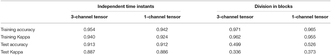
Table 1. Performance metrics obtained with CNN assuming independent time instants and division in blocks.
On the other hand, results for division in blocks were worse. In this scenario, accuracy was 0.97 and 0.49 in training and test sets when training with 3-channel tensors, respectively (Cohen's kappa of 0.96 and 0.33). Metrics when training with 1-channel tensors were similar in the training set but slightly better in the test set (accuracy of 0.52 and Cohen's kappa of 0.37), but worse compared with time independence approach. These results suggest that we are overfitting the model to the training set.
Figure 4 shows the confusion matrix obtained in the test set for both training approaches and tensor types, while Table 2 shows the accuracy, sensitivity and specificity obtained for each label when training with 1-channel tensors. In the case of time independence, accuracy ranged from 0.81 to 0.975, although it worsened to 0.43 in the case of the drivers located in the septum area (label 7, accuracy of 0.430). These results are justified by the imbalance of our dataset. Labels from 0 to 5, although their population are also imbalanced, are highly represented, but the number of samples with labels 6 and 7 is very low. Results for the CNN model trained with 3-channel tensors were slightly worse. Regarding sensitivity, the system is able to detect with high precision clinically relevant regions. Those areas where ECGI has less reconstruction capacity (like the septum area), the sensitivity is lower. However, it is essential to remark that both in clinical practice and in our database these regions present a lower probability of present drivers. Regarding specificity, obtained scores were always above 0.94.
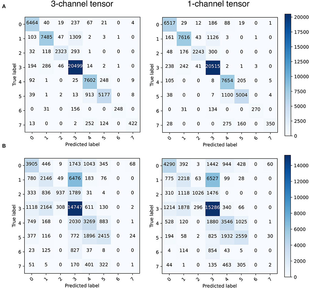
Figure 4. Confusion matrices obtained in the test set (1-channel tensor) for time independence (A) and division in blocks (B).
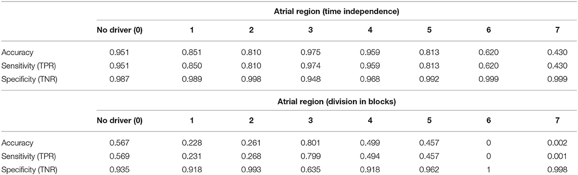
Table 2. Accuracy, sensitivity, and specificity scores obtained with 1-channel CNN assuming time independence and division in blocks (by labels, test set).
In the case of division in blocks, results were significantly worse. Highest accuracy was obtained for the label 3 (0.80), which is the one with the largest representation in the dataset. However, accuracy for the rest of labels ranged from 0.22 to 0.56, and near 0 for labels 6 and 7. The high temporal redundancy between consecutive signal samples could explain overfitting in this scenario, although the training set was previously shuffled before fitting the model. The low number of computerized AF models makes also difficult to help the CNN model to generalize. Regarding sensitivity, results were also significantly worse, although the system was able to get a sensitivity of 0.799 in the most represented atrial zone (label 3). Finally, the rate of TN is very high for every label, except for the label 3, with a specificity of 0.635.
In this second experiment, we evaluated the possibility of using pre-trained CNN models for AF driver localization, instead of using a custom CNN architecture. Models were trained with 1-channel tensors obtained with noisy BSP (SNR = 20 dB). Since pre-trained models require 3-channel tensors, we repeated the tensor twice to obtain 3-channel tensors. The custom CNN model was trained with the original 1-channel tensor.
Moreover, to assess the noise robustness of those DL models, we tested them with tensors whose associated BSP were corrupted with noise (SNR from 5 to 50 dB, in steps of 5 dB). This procedure was repeated 20 times in order to obtain test signals with different noise but same SNR. Then, the mean and SD of performance metrics were computed.
Figure 5 shows the performance metrics obtained for the test set, assuming time independence and division in blocks, for each CNN model, whereas Table 3 shows the average accuracy values for the custom CNN model and fully trained pre-trained models (SNR from 5 to 20 dB). In both cases, performance of pre-trained networks was significantly better when training the full network instead of performing a partial training (where the network was freezed except the last two convolutional layers and the fully connected ones). For time independence, average accuracy values obtained with fully trained pre-trained models ranged from 0.788 (5 dB) to 0.93 (20 dB upward), whereas the best accuracy value obtained for partially trained models was 0.90 (Xception model). Regarding average Cohen's kappa metric, it ranged from 0.72 (5dB) to 0.91 (20 dB upward) for fully-trained models, while the highest obtained score for all partially trained pre-trained models was 0.87 (Xception model).
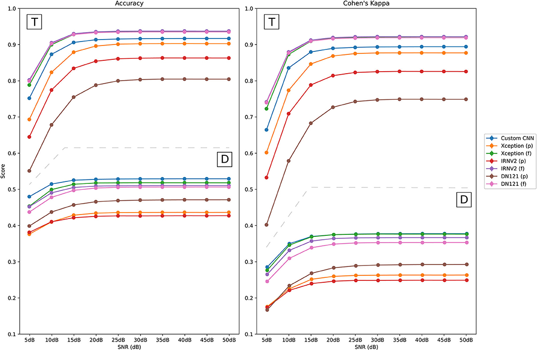
Figure 5. Performance of CNN models on noisy test signals when assuming time independence (T) and division in blocks (D). Partially trained CNN models are marked with (p), and fully trained ones are identified as (f).
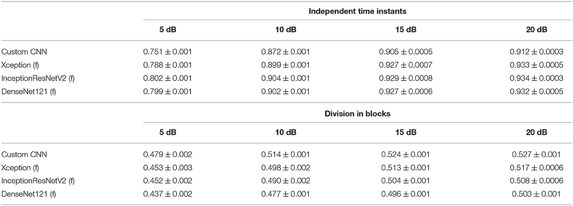
Table 3. Average accuracy values obtained for the different fully trained networks and noisy PSD (SNR = 5, 10, 15 and 20 dB, test set).
On the other hand, average accuracy values obtained for the division in blocks approach were significantly worse for all the CNN models. The best average accuracy value was 0.51 among the different pre-trained models (SNR = 20 dB upward, Xception fully trained model), whereas the best overall accuracy value was 0.527 for the custom CNN model. Both are much lower values than the ones obtained for time independence.
Regarding the performance when testing with much noisier signals, performance degraded for SNR = 5 dB, with average accuracy scores below 0.802 when assuming time independence (0.479 with division in blocks). However, it improved from SNR = 10 dB with average accuracy values over 0.87 in the time independence approach (in the division in blocks approach the best score for SNR = 10 dB was 0.51 for the custom CNN model). Additionally, SD values of the accuracy were always below 0.001, which suggests that the CNN models are robust to noise changes.
Finally, performance metrics for fully trained pre-trained models were very similar between them when assuming time independence, outperforming the custom CNN model. However, in the case of division in blocks, the custom CNN outperformed fully trained pre-trained networks, although differences between these models were very small.
The use of CNNs can help to identify target regions for ablation using body surface potential mapping, avoiding ECGI. The proposed method, which converts BSP into images, has been demonstrated to be accurate and robust to noise, i.e., the performance just degrades for very low values of SNR.
Regarding the architecture of the tensors, the 1-channel tensor-based architecture was able to obtain more accurate results than the 3-channel one, both assuming time independence or division in blocks. In relation to the training process, the single-channel tensor-based CNN model required a higher number of epochs to be fitted than in the 3-channel one. However, since each epoch is slower in the 3-channel architecture (3D matrix), the final training process becomes faster when using single-channel tensors.
Moreover, this methodology makes transfer learning very easy to apply, since it can be used to adapt much more complex pre-trained CNN models to a very specific task with promising results. However, results were significantly better when re-training the whole network (much slower procedure) than when training just the final layers. Therefore, using pre-trained models requires further research.
Although this study showed very promising results, it has several limitations that should be taken into account. The first one is the size and balance of our dataset. It is composed by 130 sets of BSP, obtained with 10 torso geometries but from only 13 AF computerized models, so the number of represented propagation patterns is low. Moreover, the distribution of drivers across the seven defined atrial regions is not balanced, i.e., there are regions that are over-represented, and performance will be worse on under-represented regions. However, we have decided to use the proposed division in seven regions because it represents a clinical-based classification of the areas where the AF drivers are more commonly found and has been already clinically used to guide AF ablation strategies demonstrating to have a clear clinical significance (Haissaguerre et al., 2014). Besides, the proposed classification method can be easily extrapolated to other atrial geometry divisions based on a higher number of smaller regions, being able to get a higher resolution in the driver classification.
Another important problem to be faced is the training approach. In this study, we first trained the models with random samples that belongs to the 13 AF models available (time independence). However, in a real situation, the DL model will have to compute a prediction with a data set that the network has never seen. Therefore, we decided to train the models with a chunk of signals of each model, while testing with the rest. In this scenario, performance substantially worsened because of the high temporal redundancy between consecutive time instants and the low number of AF models. Both facts lead to overfit to the training set, even when using tools like dropout. Using RNNs could be useful to face the redundancy problem, since they are able to extract temporal characteristics of BSP that are omitted when using CNN.
In a real scenario, assuming model independence (i.e., training with some AF models and testing with the rest) should be the way to go, but it will require the availability of a higher number of computerized models and propagation patterns. Finally, another point of future work will be applying this methodology with real patient data. However, nowadays there is a lack of gold standard for the identification of AF drivers, and there are not labeled clinical data that could help us to validate this methodology.
Some of the computerized models used in our study are publicly available at the Experimental Data and Geometric Analysis Repository (EDGAR, https://edgar.sci.utah.edu/) by the Consortium for ECG Imaging (CEI, https://www.ecg-imaging.org/). Further inquiries can be directed to the corresponding authors.
MÁC-V and OB-P: experimental setup, code implementation, and computational tests. MÁC-V, IH-R, MG, AC, and OB-P: data collecting, cleaning, and pre-processing. MÁC-V, IH-R, EM-R, MG, AC, and OB-P: manuscript preparation. All authors contributed to the article and approved the submitted version.
This work has been partially supported by: Ministerio de Ciencia e Innovación (PID2019-105032GB-I00), Instituto de Salud Carlos III, and Ministerio de Ciencia, Innovación y Universidades (supported by FEDER Fondo Europeo de Desarrollo Regional PI17/01106 and RYC2018-024346B-750), Consejería de Ciencia, Universidades e Innovación of the Comunidad de Madrid through the program RIS3 (S-2020/L2-622), EIT Health (Activity code 19600, EIT Health is supported by EIT, a body of the European Union) and the European Union's Horizon 2020 research and innovation program under the Marie Skłodowska-Curie grant agreement No. 860974.
AC, MG, and IH-R hold equity in Corify Care. AC have received honoraria from Corify Care.
The remaining authors declare that the research was conducted in the absence of any commercial or financial relationships that could be construed as a potential conflict of interest.
All claims expressed in this article are solely those of the authors and do not necessarily represent those of their affiliated organizations, or those of the publisher, the editors and the reviewers. Any product that may be evaluated in this article, or claim that may be made by its manufacturer, is not guaranteed or endorsed by the publisher.
Barr, R. C., Ramsey, M., and Spach, M. S. (1977). Relating epicardial to body surface potential distributions by means of transfer coefficients based on geometry measurements. IEEE Trans. Biomed. Eng. 24, 1–11. doi: 10.1109/TBME.1977.326201
Brooks, D. H., and Macleod, R. (1997). Electrical imaging of the heart. IEEE Signal Process. Mag. 14, 24–42. doi: 10.1109/79.560322
Bujnarowski, K., Bonizzi, P., Cluitmans, M., Peeters, R., and Karel, J. (2020). “Ct-scan free neural network-based reconstruction of heart surface potentials from ecg recordings,” in 2020 Computing in Cardiology (Rimini: IEEE), 1–4.
Cámara-Vázquez, M., Á, Oter-Astillero, A., Hernández-Romero, I., Rodrigo, M., Morgado-Reyes, E., et al. (2020). “Atrial fibrillation driver localization from body surface potentials using deep learning,” in 2020 Computing in Cardiology (Rimini,: IEEE), 1–4.
Chollet, F. (2016). Xception: Deep learning with depthwise separable convolutions. CoRR, abs/1610.02357. doi: 10.1109/CVPR.2017.195
Chugh, S. S., Havmoeller, R., Narayanan, K., Singh, D., Rienstra, M., Benjamin, E. J., et al. (2014). Worldwide epidemiology of atrial fibrillation: a global burden of disease 2010 study. Circulation 129, 837–847. doi: 10.1161/CIRCULATIONAHA.113.005119
Cuculich, P. S., Wang, Y., Lindsay, B. D., Faddis, M. N., Schuessler, R. B., Damiano, R. J., et al. (2010). Noninvasive characterization of epicardial activation in humans with diverse atrial fibrillation patterns. Circulation 122, 1364–1372. doi: 10.1161/CIRCULATIONAHA.110.945709
De Greef, Y., Schwagten, B., Chierchia, G. B., de Asmundis, C., Stockman, D., and Buysschaert, I. (2018). Diagnosis-to-ablation time as a predictor of success: early choice for pulmonary vein isolation and long-term outcome in atrial fibrillation: results from the Middelheim-PVI Registry. EP Eur. 20, 589–595. doi: 10.1093/europace/euw426
De Munck, J. (1992). A linear discretization of the volume conductor boundary integral equation using analytically integrated elements. IEEE Trans. Biomed. Eng. 39, 986–990. doi: 10.1109/10.256433
Dössel, O., Krueger, M. W., Weber, F. M., Wilhelms, M., and Seemann, G. (2012). Computational modeling of the human atrial anatomy and electrophysiology. Med. Biol. Eng. Comput. 50, 773–799. doi: 10.1007/s11517-012-0924-6
Dubois, R., Shah, A. J., Hocini, M., Denis, A., Derval, N., Cochet, H., et al. (2015). Non-invasive cardiac mapping in clinical practice: application to the ablation of cardiac arrhythmias. J. Electrocardiol. 48, 966–974. doi: 10.1016/j.jelectrocard.2015.08.028
Figuera, C., Suárez-Gutiérrez, V., Hernández-Romero, I., Rodrigo, M., Liberos, A., Atienza, F., et al. (2016). Regularization techniques for ECG Imaging during atrial fibrillation: a computational study. Front. Physiol. 7:466. doi: 10.3389/fphys.2016.00556
Fuster, V., Rydén, L. E., Cannom, D. S., Crijns, H. J., Curtis, A. B., Ellenbogen, K. A., et al. (2006). Acc/aha/esc 2006 guidelines for the management of patients with atrial fibrillation: full text. Europace 8, 651–745. doi: 10.1093/europace/eul097
García-Molla, V., Liberos, A., Vidal, A., Guillem, M., Millet, J., González, A., et al. (2014). Adaptive step {ODE} algorithms for the 3d simulation of electric heart activity with graphics processing units. Comput. Biol. Med. 44, 15–26. doi: 10.1016/j.compbiomed.2013.10.023
Guillem, M., Climent, A., Rodrigo, M., Fernández-Avilés, F., Atienza, F., and Berenfeld, O. (2016). Presence and stability of rotors in atrial fibrillation: evidence and therapeutic implications. Cardiovasc. Res. 109, 480–492. doi: 10.1093/cvr/cvw011
Gulrajani, R. (1998). The forward and inverse problems of electrocardiography. IEEE Eng. Med. Biol. 17, 84–101. doi: 10.1109/51.715491
Haissaguerre, M., Hocini, M., Denis, A., Shah, A. J., Komatsu, Y., Yamashita, S., et al. (2014). Driver domains in persistent atrial fibrillation. Circulation 130, 530–538. doi: 10.1161/CIRCULATIONAHA.113.005421
Haissaguerre, M., Hocini, M., Shah, A. J., Derval, N., Sacher, F., Jais, P., et al. (2013). Noninvasive panoramic mapping of human atrial fibrillation mechanisms: a feasibility report. J. Cardiovasc. Electrophysiol. 24, 711–717. doi: 10.1111/jce.12075
Huang, G., Liu, Z., and Weinberger, K. Q. (2016). Densely connected convolutional networks. CoRR, abs/1608.06993. doi: 10.1109/CVPR.2017.243
Koivumäki, J. T., Seemann, G., Maleckar, M. M., and Tavi, P. (2014). In silico screening of the key cellular remodeling targets in chronic atrial fibrillation. PLoS Comput. Biol. 10:e1003620. doi: 10.1371/journal.pcbi.1003620
Krizhevsky, A., Sutskever, I., and Hinton, G. E. (2017). Imagenet classification with deep convolutional neural networks. Commun. ACM. 60, 84–90. doi: 10.1145/3065386
Krummen, D. E., Baykaner, T., Schricker, A. A., Kowalewski, C. A., Swarup, V., Miller, J. M., et al. (2017). Multicentre safety of adding Focal Impulse and Rotor Modulation (FIRM) to conventional ablation for atrial fibrillation. Europace 19, 769–774. doi: 10.1093/europace/euw377
Lawson, C. L. (1984). C1 surface interpolation for scattered data on a sphere. Rocky Mountain J. Math. 14, 177–202. doi: 10.1216/RMJ-1984-14-1-177
Li, Z., Feng, X., Wu, Z., Yang, C., Bai, B., and Yang, Q. (2019). Classification of atrial fibrillation recurrence based on a convolution neural network with svm architecture. IEEE Access. 7, 77849–77856. doi: 10.1109/ACCESS.2019.2920900
Lip, G. Y., and Tse, H.-F. (2007). Management of atrial fibrillation. Lancet 370, 604–618. doi: 10.1016/S0140-6736(07)61300-2
Luongo, G., Azzolin, L., Schuler, S., Rivolta, M. W., Almeida, T. P., Martínez, J. P., et al. (2021). Machine learning enables non-invasive prediction of atrial fibrillation driver location and acute pulmonary vein ablation success using the 12-lead ECG. Cardiovasc. Digit. Health J. 2, 126–136. doi: 10.1016/j.cvdhj.2021.03.002
MacLeod, R. S., and Brooks, D. H. (1998). Recent progress in inverse problems in electrocardiology. Biol. Soc. Mag. 17, 73–83. doi: 10.1109/51.646224
McHugh, M. L. (2012). Interrater reliability: the kappa statistic. Biochem. Med. 22, 276–282. doi: 10.11613/BM.2012.031
Milanic, M., Jazbinsek, V., MacLeod, R. S., Brooks, D. H., and Hren, R. (2014). Assessment of regularization techniques for electrocardiographic imaging. J. Electrocardiol. 47, 20–28. doi: 10.1016/j.jelectrocard.2013.10.004
Narayan, S. M., Krummen, D. E., Shivkumar, K., Clopton, P., Rappel, W.-J., and Miller, J. M. (2012). Treatment of atrial fibrillation by the ablation of localized sources. J. Am. Coll. Cardiol. 60, 628–636. doi: 10.1016/j.jacc.2012.05.022
Navara, R., Leef, G., Shenasa, F., Kowalewski, C., Rogers, A. J., Meckler, G., et al. (2018). Independent mapping methods reveal rotational activation near pulmonary veins where atrial fibrillation terminates before pulmonary vein isolation. J. Cardiovasc. Electrophysiol. 29, 687–695. doi: 10.1111/jce.13446
Nygren, A., Fiset, C., Firek, L., Clark, J. W., Lindblad, D. S., Clark, R. B., et al. (1998). Mathematical model of an adult human atrial cell: the role of k+ currents in repolarization. Circ. Res. 82, 63–81. doi: 10.1161/01.RES.82.1.63
Oesterlein, T., Frisch, D., Loewe, A., Seemann, G., Schmitt, C., Dössel, O., et al. (2016). Basket-type catheters: diagnostic pitfalls caused by deformation and limited coverage. Biomed. Res. Int. 2016:5340574. doi: 10.1155/2016/5340574
Oster, H. S., and Rudy, Y. (1992). The use of temporal information in the regularization of the inverse problem in electrocardiography. IEEE Trans. Biomed. Eng. 39:65–75. doi: 10.1109/10.108129
Pan, S. J., and Yang, Q. (2009). A survey on transfer learning. IEEE Trans. Knowl. Data Eng. 22, 1345–1359. doi: 10.1109/TKDE.2009.191
Pedron-Torrecilla, J., Climent, A., Millet, J., Berne, P., Brugada, J., Brugada, R., et al. (2011). Characteristics of inverse-computed epicardial electrograms of brugada syndrome patients. Annu. Int. Conf. IEEE Eng. Med. Biol. Soc. 2011, 235–238. doi: 10.1109/IEMBS.2011.6090044
Pedrón-Torrecilla, J., Rodrigo, M., Climent, A., Liberos, A., Pérez-David, E., Bermejo, J., et al. (2016). Noninvasive estimation of epicardial dominant high-frequency regions during atrial fibrillation. J. Cardiovasc. Electrophysiol. 27, 435–442. doi: 10.1111/jce.12931
Pourbabaee, B., Roshtkhari, M. J., and Khorasani, K. (2018). Deep convolutional neural networks and learning ECG features for screening paroxysmal atrial fibrillation patients. IEEE Trans. Syst. Man Cybernet. Syst. 48, 2095–2104. doi: 10.1109/TSMC.2017.2705582
Rodrigo, M. (2016). Non-invasive identification of atrial fibrillation drivers (Ph.D. thesis). Tesis doctoral). Universitat Politècnica de València, Valencia, Espa na.
Rodrigo, M., Climent, A. M., Liberos, A., Calvo, D., Fernández-Avilés, F., Berenfeld, O., et al. (2016). Identification of dominant excitation patterns and sources of atrial fibrillation by causality analysis. Ann. Biomed. Eng. 44, 2364–2376. doi: 10.1007/s10439-015-1534-x
Rodrigo, M., Climent, A. M., Liberos, A., Fernández-Avilés, F., Berenfeld, O., Atienza, F., et al. (2017). Technical considerations on phase mapping for identification of atrial reentrant activity in direct-And inverse-computed electrograms. Circ. Arrhythm. Electrophysiol. 10:e005008. doi: 10.1161/CIRCEP.117.005008
Rodrigo, M., Guillem, M. S., Climent, A. M., Pedrón-Torrecilla, J., Liberos, A., Millet, J., et al. (2014). Body surface localization of left and right atrial high-frequency rotors in atrial fibrillation patients: a clinical-computational study. Heart Rhythm 11, 1584–1591. doi: 10.1016/j.hrthm.2014.05.013
Rottner, L., Bellmann, B., Lin, T., Reissmann, B., Tönnis, T., Schleberger, R., et al. (2020). Catheter ablation of atrial fibrillation: state of the art and future perspectives. Cardiol. Therapy 9, 45–58. doi: 10.1007/s40119-019-00158-2
Russakovsky, O., Deng, J., Su, H., Krause, J., Satheesh, S., Ma, S., et al. (2015). ImageNet large scale visual recognition challenge. Int. J. Comput. Vis. 115, 211–252. doi: 10.1007/s11263-015-0816-y
Szegedy, C., Ioffe, S., and Vanhoucke, V. (2016). Inception-v4, inception-resnet and the impact of residual connections on learning. CoRR, abs/1602.07261.
Xia, Y., Wulan, N., Wang, K., and Zhang, H. (2018). Detecting atrial fibrillation by deep convolutional neural networks. Comput. Biol. Med. 93, 84–92. doi: 10.1016/j.compbiomed.2017.12.007
Keywords: atrial fibrillation, body surface potentials, driver position, convolutional neural networks, deep learning
Citation: Cámara-Vázquez MÁ, Hernández-Romero I, Morgado-Reyes E, Guillem MS, Climent AM and Barquero-Pérez O (2021) Non-invasive Estimation of Atrial Fibrillation Driver Position With Convolutional Neural Networks and Body Surface Potentials. Front. Physiol. 12:733449. doi: 10.3389/fphys.2021.733449
Received: 30 June 2021; Accepted: 03 September 2021;
Published: 14 October 2021.
Edited by:
Stefano Schena, Johns Hopkins Medicine, United StatesReviewed by:
Laura Burattini, Marche Polytechnic University, ItalyCopyright © 2021 Cámara-Vázquez, Hernández-Romero, Morgado-Reyes, Guillem, Climent and Barquero-Pérez. This is an open-access article distributed under the terms of the Creative Commons Attribution License (CC BY). The use, distribution or reproduction in other forums is permitted, provided the original author(s) and the copyright owner(s) are credited and that the original publication in this journal is cited, in accordance with accepted academic practice. No use, distribution or reproduction is permitted which does not comply with these terms.
*Correspondence: Andreu M. Climent, YWNsaW1lbnRAaXRhY2EudXB2LmVz; Oscar Barquero-Pérez, b3NjYXIuYmFycXVlcm9AdXJqYy5lcw==
†These authors have contributed equally to this work
Disclaimer: All claims expressed in this article are solely those of the authors and do not necessarily represent those of their affiliated organizations, or those of the publisher, the editors and the reviewers. Any product that may be evaluated in this article or claim that may be made by its manufacturer is not guaranteed or endorsed by the publisher.
Research integrity at Frontiers
Learn more about the work of our research integrity team to safeguard the quality of each article we publish.