 Jean Bonnemain
 Luca Pegolotti
 Lucas Liaudet
 Simone Deparis
94% of researchers rate our articles as excellent or good
Learn more about the work of our research integrity team to safeguard the quality of each article we publish.
Find out more
BRIEF RESEARCH REPORT article
Front. Physiol. , 11 September 2020
Sec. Computational Physiology and Medicine
Volume 11 - 2020 | https://doi.org/10.3389/fphys.2020.01086
The evaluation of cardiac contractility by the assessment of the ventricular systolic elastance function is clinically challenging and cannot be easily obtained at the bedside. In this work, we present a framework characterizing left ventricular systolic function from clinically readily available data, including systemic and pulmonary arterial pressure signals. We implemented and calibrated a deep neural network (DNN) consisting of a multi-layer perceptron with 4 fully connected hidden layers and with 16 neurons per layer, which was trained with data obtained from a lumped model of the cardiovascular system modeling different levels of cardiac function. The lumped model included a function of circulatory autoregulation from carotid baroreceptors in pulsatile conditions. Inputs for the DNN were systemic and pulmonary arterial pressure curves. Outputs from the DNN were parameters of the lumped model characterizing left ventricular systolic function, especially end-systolic elastance. The DNN adequately performed and accurately recovered the relevant hemodynamic parameters with a mean relative error of less than 2%. Therefore, our framework can easily provide complex physiological parameters of cardiac contractility, which could lead to the development of invaluable tools for the clinical evaluation of patients with severe cardiac dysfunction.
Heart failure corresponds to a clinical syndrome with a wide spectrum of symptoms, ranging from dyspnea and exercise intolerance to cardiogenic shock. It is caused by structural or functional cardiac abnormalities that result in low cardiac output, i.e., the inability of the heart to provide sufficient blood flow to satisfy the metabolic needs of the organism (Metra and Teerlink, 2017). It affects approximately 2% of the population, with a lifetime risk of developing heart failure of 20%, and a 5-years mortality of about 50% (Yancy et al., 2013). In the intensive care unit (ICU), cardiogenic shock represents 6% of admission, with an in-ICU mortality as high as 50% (Puymirat et al., 2017).
Evaluation of cardiac function is of crucial importance since it directly impacts treatment and therefore prognosis. In particular, the early and repeated evaluation of the left ventricular function is a key factor to guide therapies. This is particularly relevant in the ICU setting, where hemodynamic changes in unstable patients can occur rapidly (minutes). The aim of hemodynamic monitoring is therefore to accurately and rapidly identify changes in order to adapt treatment.
Hemodynamic assessment of cardiogenic shock is nowadays multimodal and includes clinical evaluation and paraclinical examination. Echocardiography for this situation is currently the cornerstone tool since it provides a complete evaluation of cardiac function and structure and can also predict response to treatment, in particular fluid-responsiveness (Vieillard-Baron et al., 2019). However, this examination is time- and resources-consuming (although new sensor technology may reduce the costs of these devices), hence evaluation based only on echocardiography may result in delays in management. Moreover, it cannot be used in a continuous manner. Other methods, either invasive or non-invasive, allow to indirectly assess cardiac output and volumes (Alhashemi et al., 2011; Monnet and Teboul, 2017; Nguyen and Squara, 2017).
Although these tools provide accurate estimates of ventricular function, evaluation of cardiac mechanics is fully characterized using the measure of pressure and volume of the ventricle during the entire cardiac cycle. From these values one can establish the ventricular pressure-volume diagram and determine the end-systolic and end-diastolic pressure-volume relationships. The former permit the determination of ventricular end-systolic elastance (Ees), a load-independent measurement of ventricular contractility (Burkhoff et al., 2005; Naeije and Manes, 2014). Nowadays these measurements require invasive techniques only available in the catheterization laboratory (Bonnet et al., 2017). Non-invasive methods have been developed, including magnetic resonance imaging (Bastos et al., 2019), or real-time three dimensional echocardiography (Seemann et al., 2019), but these cannot be easily implemented in the daily clinical practice.
To circumvent the drawbacks of these different methods, we aimed at developing a framework to characterize parameters of ventricular systolic function from easily accessible clinical data, namely systemic and pulmonary arterial pressures. The gold standard for such measurements is the use of invasively inserted intravascular catheters in the radial or femoral artery (systemic arterial pressure), or the pulmonary artery (pulmonary artery pressure). To obtain accurate pressure values, the measurements must be done at end-expiration and in the supine position, with standard zero reference at the level of the right atrium. Some variability of intravascular pressure measurement may still occur as a consequence of over- or underdamping of the signal (Romagnoli et al., 2014). We implemented and calibrated a deep neural network (DNN)—trained with data obtained from a lumped model of the cardiovascular system (Shi et al., 2011), as developed by Ursino (1998)—to model different levels of severity of left ventricular systolic dysfunction. This DNN takes, as input, systemic and pulmonary arterial pressure signals and returns, as output, the parameters of the lumped model that characterize left ventricular function, in particular Ees. The inputs are relevant measurable clinical values, whereas the predicted outputs—as mentioned above—cannot be easily evaluated in clinical practice; these are in turn provided to the 0D model in order to recover all other clinical values, especially the ventricular pressure-volume curves.
The role of the proposed DNN is to solve an inverse problem which maps some of the outputs of the 0D model (i.e., systemic and pulmonary arterial pressures) to its underlying parameters. Of note, previous investigators, (Pennati et al., 1997; Pant et al., 2016; Schiavazzi et al., 2017) have proposed alternate methods for parameter identification of lumped parameter models in other physiological conditions, such as single-ventricle physiology with valve dysfunction (Pant et al., 2016). In this paper, we present a novel deep-learning-based approach to solve this issue.
In this section, we focus on the online pipeline of our method (i.e., the prediction procedure) which is depicted in Figure 1, whereas the training process is described in section 2.3 for general DNNs and section 2.4 for our specific application. Input parameters were systemic and pulmonary arterial pressure curves. Theses curves are represented in the frequency domain by their Fourier coefficients. As explained in more detail in section 2.4, the Fourier coefficients were subsequently arranged in a three-dimensional tensor which served as input for the DNN. The output of the DNN were the four parameters characterizing left ventricular function in the 0D model, namely Emax,lv, Emaxlv,0, GEmax,lv, and kE,lv (see section 2.2 for more details). In the last step, the predicted parameters were provided to the 0D model to simulate and recover all the other values.
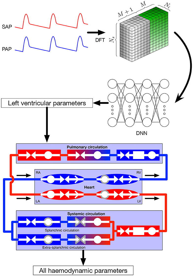
Figure 1. Global framework. Input parameters, systemic and pulmonary arterial curves are represented in the frequency domain and then given to the DNN, that itself returns the left ventricular parameters of the 0D model. These parameters are given to the 0D model, allowing to recover numerous hemodynamic values. Symbols in the 0D model are: circles: compliance; facing triangles (double arrows): resistance; rectangles: inertance; single white arrows in heart chambers: cardiac valves; gray contour: elements affected by autoregulation; red elements: oxygenated blood, blue elements: deoxygenated blood. SAP, systemic arterial pressure; PAP, pulmonary arterial pressure; DFT, discrete Fourier transform, providing the coefficients ak and bk; DNN, deep neural network; RA, right atrium; RV, right ventricle; LA, left atrium; LV, left ventricle.
The lumped model of the cardiovascular system has been extensively described in the original paper by Ursino (1998). The model provides a mathematical description of the entire cardiovascular system with time-varying elastance of the left and right ventricles. It also includes the afferent carotid baroreceptor pathway, the sympathetic and vagal efferent activities, the splanchnic and extrasplanchnic systemic circulation, and the pulmonary circulation. A representation of the model is presented at the bottom of Figure 1. For each of the vascular i-compartment, mass and momentum conservation are given by, respectively:
and
where Vi is the volume of the i-compartment, Qin and Qout the inflow and outflow rate, Pin and Pout the inlet and outlet pressure, Ri the resistance, and Li the inertance. The pressure and flow relationship reads
Inertance is taken into account for arterial compartments where acceleration of blood is significant, while neglected for the other ones. Valve opening is determined by its pressure gradient across the valve, i.e., it opens when Pin > Pout. Left and right ventricle contractility is modeled as a time-varying elastance. Efferent pathways act on several parameters, namely heart period, left and right ventricle contractility, unstressed volumes (defined as the volume when pressure is equal to zero), and both splanchnic and extrasplanchnic peripheral artery resistance. Parameters affected by autoregulation are surrounded by a gray line in Figure 1.
In a previous work (Bonnemain et al., 2013), we modified the model to account for left ventricular systolic failure at different levels of severity and validated it with clinical data. To reproduce various degrees of left ventricular systolic failure, we varied the following parameters:
• Emax,lv [mmHg/ml], reference value of the ventricle elastance,
• Emaxlv,0 [mmHg/ml], reference value of the ventricle elastance in absence of autoregulation,
• GEmax,lv [mmHg/ml/(spikes/s)], maximum baroreceptor gain,
• kE,lv [1/ml], steepness of the pressure-volume curve.
Figure 2 shows left ventricular pressure-volume loops at different degrees of severity of heart failure. All other haemodynamic values are presented in Bonnemain et al. (2013). For each compartment, pressure, volume and flow can be extracted; it is therefore straight-forward to retrieve the ventricular pressure-volume curves.
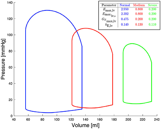
Figure 2. Pressure-volume diagrams for different degrees of systolic heart failure and their corresponding parameters in the 0D model.
The term machine learning is typically used to indicate a family of algorithms and methods which, broadly speaking, are capable of identifying structures and patterns in complex and (usually) high-dimensional information. Due to the abundance of data obtained during the last decade and the ever increasing computational power of processors, graphics processing units (GPUs) and supercomputers, these methods have gained particular attention in all the fields of medicine (Komorowski et al., 2018; McKinney et al., 2020).
DNNs are a class of data-hungry machine learning algorithms notably suited for classification and regression tasks. They are used to approximate unknown mappings f(·) of the form y = f(x; ω), where x and y are input and output of the model, respectively, and ω indicates a set of parameters of the network. The function f(·), which, in reality, can be as general as possible, is represented in DNNs as a composition of easily computable parameterized functions f1, f2, …, fl (where l is the number of layers of the network), i.e., f = fl ◦ … ◦ f2 ◦ f1. In this work, we focused on the most basic type of DNNs, i.e., multi-layer perceptrons, which, despite their simple structure, have been mathematically proven to satisfy desirable approximation properties. In particular, multi-layer perceptrons with one hidden layer or more are universal approximators, see e.g., (Cybenko, 1988; Mhaskar, 1993). In contrast to more advanced architectures (e.g., convolutional neural networks), multi-layer perceptrons are solely based on a sequence of fully-connected layers of the form
where the subscript i refers to the ith layer of the network, xi = yi−1 is the corresponding input, Wi and bi are a weight matrix and a bias vector, and σi is a non-linear activation function. Among the most common activation functions are e.g., the rectifier linear unit ReLU(x) = max(0, x), sigmoid(x) = 1/(1 + exp(−x)), and tanh(x). In this paper, we consider the ReLU and sigmoid activation functions for the hidden (i.e., f1, …, fl−1) and output (i.e., fl) layers, respectively. The weight matrix Wi and the bias vector bi represent the parameters ωi of the ith layer. In order to find an appropriate numerical value of the parameters ωi, for each i = 1, 2, …, l, the DNN has to be trained on a set of input-output pairs which constitute the so called training dataset. The ultimate goal of the training process is to find ω = {ω1, ω2, …, ωl} such that the DNN f(·, ω) performs a “good” fitting on Q, i.e., f(xk, ω) ≈ yk for every k = 1, 2, …, nt. This is typically done by introducing a loss function acting on the training dataset and by minimizing it by means of optimization algorithms (usually, gradient or stochastic gradient descent). For a complete review of DNNs and their optimization, we refer the reader to Goodfellow et al. (2016).
In the data generation phase, the 0D model described in section 2.2 is solved Ns times by randomly sampling Emax,lv, Emaxlv,0, GEmax,lv, and kE,lv. Specifically, we determined for each of these parameters a range of physiological or pathological (severe heart failure) values; for details about these ranges see (Bonnemain et al., 2013). Upper and lower bounds are reported in Figure 2. Each training sample was generated from the 0D model, by assigning a random individual value (drawn from a uniform distribution defined on the corresponding admissible range) for each of the four parameters of interest, and by keeping constant all the other parameters of the 0D model. Other parameters include values of resistance, compliance, unstressed volume, inertance, as well as values describing heart function, and values related to autoregulation, as presented in detail by Ursino (1998). This approach allows generating a dataset which includes a rich representation of all possible pathological conditions leading to left heart failure. Regarding sampling strategies, owing to the negligible computational cost required the generate each random sample, we did not consider alternative sampling strategies (e.g., Latin Hypercube or orthogonal sampling). The output of the 0D model comprises multiple time dependent one-dimensional signals. We focused only on quantities that are easy to measure in the clinical practice, such as systemic arterial pressure and pulmonary arterial pressure. Let us denote (0, T) the time interval over which the simulation of the 0D model is performed, t1 = 0, …, tnt = T a set of timesteps such that the timestep size Δt = tm + 1 − tm is constant for all m = 1, …, nt, and the value of the ith quantity of interest (e.g., systemic or pulmonary arterial pressure) of the kth sample at timestep tm. In order to better capture the time component of the quantity of interest, we decided to operate on its representation in the frequency domain. More precisely, we computed the Discrete Fast Fourier Transform (DFFT) of the signal and we recovered the coefficients and such that, for all k = 0, …, nt,
where M = nt/2 and ω = 2π/T. We note that Equation (5) must be slightly modified to account for the case of nt odd; we refer to Quarteroni et al. (2014) for details. We introduce for sake of clarity the vector , i.e., the vector containing all the 2M + 1 Fourier coefficients. In this work we selected the first 5% of Fourier coefficients, i.e., M = 5. Cutting higher modes allows to eliminate noise without loosing information. We studied the influence of the number of Fourier coefficients used for the DNN input on the DNN performance. Data from these studies are provided in Supplementary Data Sheet 2. Overall, results indicate that the best accuracy of the DNN is obtained using M = 5 (11 Fourier coefficients).
The training dataset Q for the DNN is composed of pairs {xk, yk}, k = 1, …, Ns, where , Ni being the number of desired input signals selected from the output of the 0D model, and . In our implementation, the input data is organized in a three-dimensional tensor with dimensions Ns × Ni × (2M + 1) as depicted in Figure 1. Therefore, the forward pass of the DNN consists in mapping the frequency coefficients of a handful of time dependent signals—in our case, systemic and pulmonary arterial pressure—to the corresponding values of the hidden parameters of the 0D model (as already mentioned in section 1, the DNN aims at solving an inverse problem). Regarding the choice of loss function , in this work we focused on the mean squared error , which is well-suited to regression tasks.
The 0D model was implemented in the Modelica language1, a non-proprietary, object-oriented, equation based language which conveniently models complex physical systems. We used OpenModelica2 as a modeling and simulation environment. The DNN was implemented using TensorFlow3. Discrete fast Fourier transform computation and statistical analysis were performed with Matlab4.
As described in section 2.4, samples were generated from the 0D model; 5% of these were reserved to the test set, which was employed to evaluate the performance of the trained network. Of the 95% samples remaining, 80% represented the train set and 20% the validation set. After considering several DNN architectures, we opted for a multi-layer perceptron with 4 fully connected hidden layers featuring 16 neurons per layer. Our choice was driven by the value of loss function achieved during training and by the absence of overfitting (which occurs whenever the error on the train set is considerably smaller than that on the validation set); in cases of architectures achieving similar performance, we chose the network composed of the smallest number of neurons. All the data regarding the considered DNN architectures and the relative performances can be found in the Supplementary Data Sheet 1. The learning rate is set at a value of 0.001. The Adam optimization algorithm was used to update the network weights during training. In Figure 3 we report the DNN performance for the 4 predicted parameters on the test set. Each graph represents the plotting of values of real parameter (x-axis) and the predicted parameter (y-axis). We note that the optimal prediction corresponds to the bisector. The architecture shows good accuracy especially for Emax,lv, Emaxlv,0, and kE,lv. In contrast, the prediction of GEmax,lv appeared less accurate, which suggests that the 0D model is significantly less sensitive to this parameter.
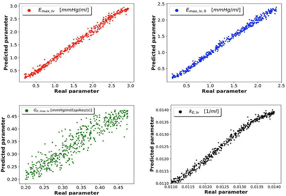
Figure 3. DNN performance for the 4 predicted parameters. Each plot compares the real parameter on the x-axis with the predicted one with the DNN on the y-axis. Emax,lv [mmHg/ml]: reference value of ventricle elastance, Emaxlv,0 [mmHg/ml]: reference value of ventricle elastance in absence of autoregulation, GEmax,lv [mmHg/ml/(spikes/s)]: maximum baroreceptor gain, kE,lv [1/ml]: steepness of the pressure-volume curve.
To support this hypothesis, we performed a sensitivity analysis of the output of the 0D model with respect to small variations of the 4 parameters. The mean value of parameter P is given by Pmean = (Pmin + Pmax)/2, where Pmin and Pmax are the lower and upper bounds depicted in Figure 2. For each parameter P, we run a set of 100 simulations by assigning the value P = Pmean(1 + ϵN(0, 1)), where ϵ = 0.01 and N(0, 1) is a normal distribution with 0 mean and a standard deviation equal to 1, while keeping the other 3 parameters constant and equal to their respective mean values. The results are reported in Table 2. The output of interest shows a noticeably lower standard deviation with respect to small variations of GEmax,lv, highlighting a lower sensibility of the 0D model for this parameter.
As depicted in Figure 1 and described in section 2.1, the main objective of our study was to recover a wealth of haemodynamic values from systemic and pulmonary arterial pressure signals. Table 1 shows the results of the 0D model simulations solved for the real and predicted parameters. Specifically, the 0D model was run for each 4-parameters set of the test set (5% of total samples, i.e., 500 samples), both with the real and the predicted parameters. Relevant haemodynamic values were extracted and compared. These values were: systemic and pulmonary pressures (mean, systolic, and diastolic), heart rate, left ventricular ejection fraction, left ventricular end-diastolic and end-systolic volumes, cardiac index, and pulmonary capillary pulmonary wedge pressure. Minimal, maximal, mean, and standard deviation of the real and predicted values were calculated. The calculated difference between real and predicted values was defined as the error, for which standard deviation with 95% confidence interval were computed. All values are reported in Table 1.
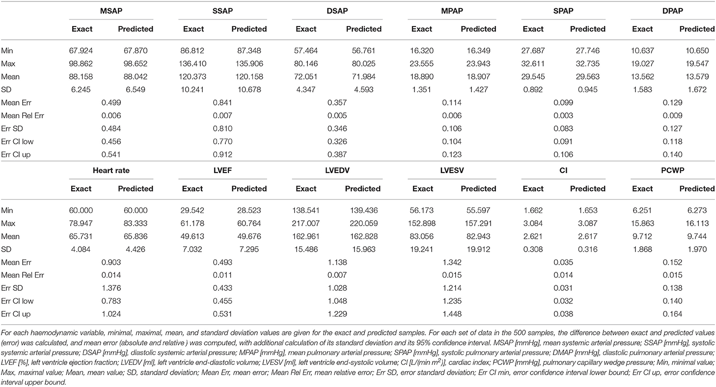
Table 1. Comparison between real and DNN-predicted hemodynamic data on the test set (500 samples).
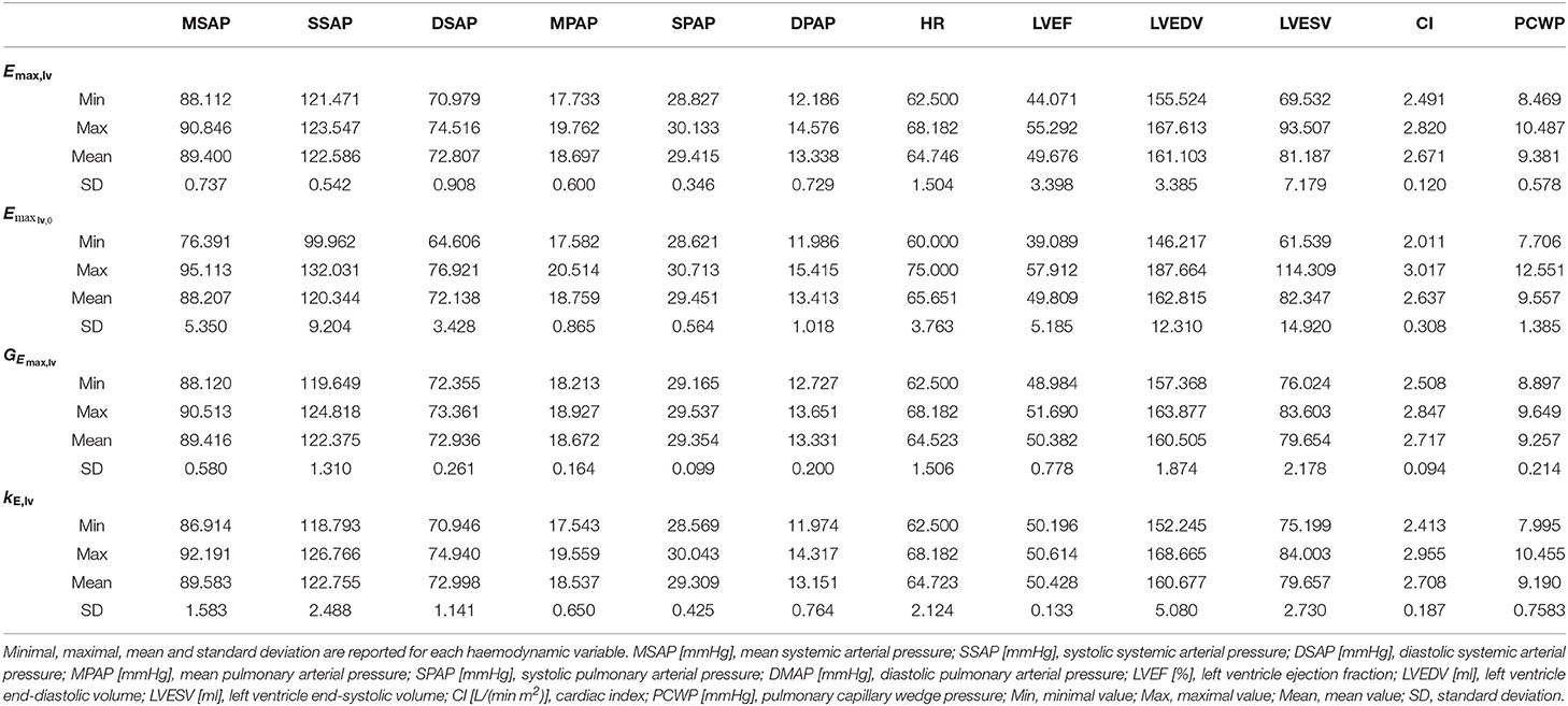
Table 2. Sensitivity analysis for the 4 predicted parameters, performed as described in section 3.
Our test set included haemodynamic values spanning a range of clinical situation from normal physiology to severe heart failure. Overall our results indicate an excellent correlation between real and predicted values, with mean relative error never superior to 2%, and a narrow 95%-confidence interval. The accuracy of this model is relevant to the clinical setting, where these hemodynamic variables are susceptible to show wide variations.
Furthermore, the small error in our model should be regarded as perfectly acceptable, when considering the variability of intravascular pressure measurements in the clinical setting, notably related to underdamping and resonance phenomena (Romagnoli et al., 2014). The same is true for clinical measurements of ventricular volumes (Bastos et al., 2019). With respect to ventricular ejection fraction, it is worth mentioning that its measurement by standard modern techniques (cardiac computerized tomography, radionucleotide and invasive ventriculography, echocardiography or magnetic resonance imaging) presents a bias of less than 5% (Pickett et al., 2015), which reinforces the relevance of our model, which leads to a relative error smaller than 2%. Finally, new devices and non-invasive approaches for continuous pressure measurement may broaden the applicability of the presented framework (Proena et al., 2016), while new methods for haemodynamic monitoring could provide innovative perspectives (Pour-Ghaz et al., 2019).
Our model appears slightly better to predict pressures than other parameters, which may reflect the fact that the DNN takes pressure, but not volumes values, as input. In addition, with respect of heart rate, it can be noticed that minimal predicted and real values were identical (60/min), which simply reflects the lowest boundary of this parameter in the 0D model.
We acknowledge the three following limitations in our study. First, our model is adapted to the pathophysiology of left heart failure, and therefore cannot apply to other condition of cardiac failure, such as right heart dysfunction. Secondly, we choose to focus only on 4 parameters of interest. Therefore, it is likely that including additional parameters (for instance a resistance parameter associated with vascular dysfunction) could have affected the resulting accuracy of the network. Third, even though the 0D model includes a component of autoregulation, it does not take into account respiratory physiological variables, which may significantly influence cardiac function (concept of heart-lung interactions), notably in the context of mechanical ventilation, which is frequently provided in patients with severe cardiac failure. Fourth, our study used exclusively synthetic data. Using real patients data (possibly affected by noise) to validate our framework will be essential for its applicability in the clinical setting, and such validation will be the matter of future investigations. Furthermore, we cannot rule out that using real clinical data could affect the ability to train the proposed network, an issue that will require additional studies.
In this work we presented a framework that allows to predict, from physiological data (systemic and pulmonary arterial pressure signals), various parameters of left ventricular function and other haemodynamic variables. The 0D model used to train the DNN in our study allows to describe a wide spectrum of pathophysiological alterations pertaining to left heart failure. In turn, the DNN displayed remarkable accuracy to recover relevant haemodynamic parameters.
Our study represents a first step toward the development of automated tools providing helpful information on heart function. For instance, the application of our framework could assist in the real time detection of left ventricular dysfunction, especially in ICU patients, who are subject to continuous monitoring of intravascular pressures. Also, our tool could be useful to assess the left ventricular function during mechanical circulatory support, such as left ventricular assist device (LVAD) or veno-arterial extracorporeal membrane oxygenation (ECMO).
Future studies, that will validate the model with patient related data, will be necessary for the clinical implementation of our tool. Moreover, our framework will be of great interest for the future extensions of the 0D model to other circulatory pathologies or heart disease as well as to mechanical circulatory support.
The raw data supporting the conclusions of this article will be made available by the authors, without undue reservation. Implementation of the lumped parameter model can be found at: https://bitbucket.org/jbonnema/lumped_parameter_model/src/master/.
JB contributed to the design and the implementation of the research, to the analysis of results and to the writing of the manuscript. LP contributed to the design and the implementation of the research, and to the writing of the manuscript. SD contributed to the design of the research, to the analysis of the results, and to the writing of the manuscript. LL contributed to the analysis of the research and to the writing of the manuscript. All authors contributed to the article and approved the submitted version.
This work was supported in part by a grant from the Swiss National Fund for Scientific Research to SD (200021E-168311) and in part by Departmental funds (Fondation des soins intensifs et Centre des brûlés du CHUV).
The authors declare that the research was conducted in the absence of any commercial or financial relationships that could be construed as a potential conflict of interest.
The Supplementary Material for this article can be found online at: https://www.frontiersin.org/articles/10.3389/fphys.2020.01086/full#supplementary-material
Alhashemi, J. A., Cecconi, M., and Hofer, C. K. (2011). Cardiac output monitoring: an integrative perspective. Crit. Care 15:214. doi: 10.1186/cc9996
Bastos, M. B., Burkhoff, D., Maly, J., Daemen, J., Uil, C. A. d., Ameloot, K., et al. (2019). Invasive left ventricle pressure volume analysis: overview and practical clinical implications. Eur. Heart J. 41, 1286–1297. doi: 10.1093/eurheartj/ehz552
Bonnemain, J., Malossi, A. C. I., Lesinigo, M., Deparis, S., Quarteroni, A., and Segesser, L. K. v. (2013). Numerical simulation of left ventricular assist device implantations: comparing the ascending and the descending aorta cannulations. Med. Eng. Phys. 35, 1465–1475. doi: 10.1016/j.medengphy.2013.03.022
Bonnet, B., Jourdan, F., Cailar, G. d., and Fesler, P. (2017). Noninvasive evaluation of left ventricular elastance according to pressure-volume curves modeling in arterial hypertension. Am. J. Physiol. Heart Circ. Physiol. 313, H237–H243. doi: 10.1152/ajpheart.00086.2017
Burkhoff, D., Mirsky, I., and Suga, H. (2005). Assessment of systolic and diastolic ventricular properties via pressure-volume analysis: a guide for clinical, translational, and basic researchers. Am. J. Physiol. Heart Circ. Physiol. 289, H501–H512. doi: 10.1152/ajpheart.00138.2005
Cybenko, G. (1988). Continuous Valued Neural Networks With Two Hidden Layers Are Sufficient. Technical report. Medford, MA: Department of Computer Science, Tufts University.
Goodfellow, I., Bengio, Y., Courville, A., and Bengio, Y. (2016). Deep learning, Vol. 1. Cambridge: MIT Press.
Komorowski, M., Celi, L. A., Badawi, O., Gordon, A. C., and Faisal, A. A. (2018). The Artificial Intelligence Clinician learns optimal treatment strategies for sepsis in intensive care. Nat. Med. 24, 1716–1720. doi: 10.1038/s41591-018-0213-5
McKinney, S. M., Sieniek, M., Godbole, V., Godwin, J., Antropova, N., Ashrafian, H., et al. (2020). International evaluation of an AI system for breast cancer screening. Nature 577, 89–94. doi: 10.1038/s41586-019-1799-6
Metra, M., and Teerlink, J. R. (2017). Heart failure. Lancet 390, 1981–1995. doi: 10.1016/s0140-6736(17)31071-1
Mhaskar, H. N. (1993). Approximation properties of a multilayered feedforward artificial neural network. Adv. Comput. Math. 1, 61–80. doi: 10.1007/2FBF02070821
Monnet, X., and Teboul, J.-L. (2017). Transpulmonary thermodilution: advantages and limits. Crit. Care 21:147. doi: 10.1186/s13054-017-1739-5
Naeije, R., and Manes, A. (2014). The right ventricle in pulmonary arterial hypertension. Eur. Respir. Rev. 23, 476–487. doi: 10.1183/09059180.00007414
Nguyen, L. S., and Squara, P. (2017). Non-invasive monitoring of cardiac output in critical care medicine. Front. Med. 4:200. doi: 10.3389/fmed.2017.00200
Pant, S., Corsini, C., Baker, C., Hsia, T.-Y., Pennati, G., Vignon-Clementel, I. E., et al. (2016). Data assimilation and modelling of patient-specific single-ventricle physiology with and without valve regurgitation. J. Biomech. 49, 2162–2173. doi: 10.1016/j.jbiomech.2015.11.030
Pennati, G., Migliavacca, F., Dubini, G., Pietrabissa, R., and Leval, M. R. D. (1997). A mathematical model of circulation in the presence of the bidirectional cavopulmonary anastomosis in children with a univentricular heart. Med. Eng. Phys. 19, 223–234. doi: 10.1016/s1350-4533(96)00071-9
Pickett, C. A., Cheezum, M. K., Kassop, D., Villines, T. C., and Hulten, E. A. (2015). Accuracy of cardiac CT, radionucleotide and invasive ventriculography, two- and three-dimensional echocardiography, and SPECT for left and right ventricular ejection fraction compared with cardiac MRI: a meta-analysis. Eur. Heart J. Cardiovasc. Imaging 16, 848–852. doi: 10.1093/ehjci/jeu313
Pour-Ghaz, I., Manolukas, T., Foray, N., Raja, J., Rawal, A., Ibebuogu, U. N., et al. (2019). Accuracy of non-invasive and minimally invasive hemodynamic monitoring: where do we stand? Ann. Transl. Med. 7:421. doi: 10.21037/27445
Proena, M., Braun, F., Sol, J., Adler, A., Lemay, M., Thiran, J.-P., et al. (2016). Non-invasive monitoring of pulmonary artery pressure from timing information by EIT: experimental evaluation during induced hypoxia. Physiol. Meas. 37, 713–726. doi: 10.1088/0967-3334/37/6/713
Puymirat, E., Fagon, J. Y., Aegerter, P., Diehl, J. L., Monnier, A., HauwBerlemont, C., et al. (2017). Cardiogenic shock in intensive care units: evolution of prevalence, patient profile, management and outcomes, 19972012. Eur. J. Heart Fail. 19, 192–200. doi: 10.1002/ejhf.646
Quarteroni, A., Saleri, F., and Gervasio, P. (2014). Scientific Computing with MATLAB and Octave. Berlin: Springer.
Romagnoli, S., Ricci, Z., Quattrone, D., Tofani, L., Tujjar, O., Villa, G., et al. (2014). Accuracy of invasive arterial pressure monitoring in cardiovascular patients: an observational study. Crit. Care 18:644. doi: 10.1186/s13054-014-0644-4
Schiavazzi, D. E., Baretta, A., Pennati, G., Hsia, T., and Marsden, A. L. (2017). Patient-specific parameter estimation in single-ventricle lumped circulation models under uncertainty. Int. J. Numer. Methods Biomed. Eng. 33:e02799. doi: 10.1002/cnm.2799
Seemann, F., Arvidsson, P., Nordlund, D., Kopic, S., Carlsson, M., Arheden, H., and Heiberg, E. (2019). Noninvasive quantification of pressure-volume loops from brachial pressure and cardiovascular magnetic resonance. Circ. Cardiovasc. Imaging 12:e008493. doi: 10.1161/CIRCIMAGING.118.008493
Shi, Y., Lawford, P., and Hose, R. (2011). Review of zero-D and 1-D models of blood flow in the cardiovascular system. Biomed. Eng. Online 10:33. doi: 10.1186/1475-925x-10-33
Ursino, M. (1998). Interaction between carotid baroregulation and the pulsating heart: a mathematical model. Am. J. Physiol. Heart Circ. Physiol. 275, H1733–H1747. doi: 10.1152/ajpheart.1998.275.5.h1733
Vieillard-Baron, A., Millington, S. J., Sanfilippo, F., Chew, M., Diaz-Gomez, J., McLean, A., et al. (2019). A decade of progress in critical care echocardiography: a narrative review. Intens. Care Med. 45, 770–788. doi: 10.1007/s00134-019-05604-2
Keywords: heart failure, hemodynamics, deep neural network, cardiovascular modeling, blood flow model, machine learning
Citation: Bonnemain J, Pegolotti L, Liaudet L and Deparis S (2020) Implementation and Calibration of a Deep Neural Network to Predict Parameters of Left Ventricular Systolic Function Based on Pulmonary and Systemic Arterial Pressure Signals. Front. Physiol. 11:1086. doi: 10.3389/fphys.2020.01086
Received: 27 June 2020; Accepted: 06 August 2020;
Published: 11 September 2020.
Edited by:
Stephen John Payne, University of Oxford, United KingdomReviewed by:
Daniele E. Schiavazzi, University of Notre Dame, United StatesCopyright © 2020 Bonnemain, Pegolotti, Liaudet and Deparis. This is an open-access article distributed under the terms of the Creative Commons Attribution License (CC BY). The use, distribution or reproduction in other forums is permitted, provided the original author(s) and the copyright owner(s) are credited and that the original publication in this journal is cited, in accordance with accepted academic practice. No use, distribution or reproduction is permitted which does not comply with these terms.
*Correspondence: Jean Bonnemain, amVhbi5ib25uZW1haW5AY2h1di5jaA==
†These authors have contributed equally to this work
Disclaimer: All claims expressed in this article are solely those of the authors and do not necessarily represent those of their affiliated organizations, or those of the publisher, the editors and the reviewers. Any product that may be evaluated in this article or claim that may be made by its manufacturer is not guaranteed or endorsed by the publisher.
Research integrity at Frontiers
Learn more about the work of our research integrity team to safeguard the quality of each article we publish.