Topological weak-measurement-induced geometric phases revisited

We present an analytical and numerical study of a class of geometric phase induced by weak measurements. In particular, we analyze the dependence of the geometric phase on the winding ($W$) of the polar angle ($\phi$), upon a sequence of $N$ weak measurements of increased magnitude $(c)$, resulting in the appearance of a multiplicity of critical measurement-strength parameters where the geometric phase makes a $|\pi |$ discrete jump. Adding to the novelty of our approach, we not only analyze the weak-measurement-induced geometric phase by a full analytic derivation, valid in the quasi-continuous limit $(N\to \infty )$, but also we analyze the induced geometric phase numerically, thus enabling us to unravel the finite-$N$ interplay of the geometric phase with the measurement-strength parameter, and its stability to perturbations in the measurements protocol.

1 Introduction

When a quantum system undergoes adiabatic cycling, its state can become quantifiable based solely on its closed path in parameter space [1]. Conversely, a cyclic series of quantum observations can create a geometric phase. As reported in Gebhart et al. [2], for closed trajectories, upon the application of a series of steering weak measurements, a topological transition may occur in the mapping between the measurement sequence and the geometric phase, when the measurement strength is changed.

Despite the fact that overall quantum phases cannot be fully determined, when the quantum system is driven slowly over a cycle returning to its starting condition, the accumulated phase becomes gauge invariant and can be measured. As originally pointed out by Sir. M. V. Berry [3], this is a geometric phase $(X)$ in that it is dependent on characteristics of the closed trajectory in parameter space, rather than on process dynamics. Geometric phases can be held responsible for a number of situations: they can modify material properties in solids, such as conductivity in graphene [4], they can trigger the emergence of surface edge-states in topological insulators, whose surface electrons experience a geometric phase [5], they can modify the outcome of molecular chemical reactions [6], and they can affect electronic properties of matter [7]. Furthermore, understanding various physical phenomena [8–10], defining fractional statistics anyonic quasiparticles [11–13], and identifying topological invariants for quantum Hall phases [14], superconductors [15, 16], or quantitative characterizations of topological insulators via the Zak phase [17, 18], as well as underpinning holonomic and topological signatures in photonic systems [19–23], are all made possible by geometric phases.

A class of geometric phase, resulting from the outcome of a series of intense (projective) measurements that operate on the system and produce certain measurement read-outs, is the Pancharatnam phase [24]. Optical investigations that monitor the Pancharatnam phase caused by polarizer sequences have readily been reported [25]. Notwithstanding the fact that incoherent measurement processes are generally involved, such a phase may be reliably detected. A general series of measurements is by its very nature stochastic. Thus, based on the sequences of measurement readouts linked to the relevant probabilities, one may expect a distribution of measurement-induced geometric phases. The induced evolution is entirely predictable for a quasi-continuous series of strong measurements $(N\to \infty )$ because of the dynamical quantum Zeno effect [26].

In this paper, we present an analytical and numerical study of a novel type of geometric phase induced by weak measurements. Weak measurement is a robust measurement procedure enabling continuous monitoring of the evolution of a quantum state with minor disturbance or system back-action, which has been successfully implemented experimentally in the context of dynamic control of numerous quantum systems [27–29]. In contrast to PNAS 2020 [2], the originality of our approach consists in considering the dependence of the geometric phase on the winding $W$ of the polar angle $\phi$, which quantifies the number of full $2\pi$-turns the trajectory makes until it closes its path, returning to its original state. This is accomplished by setting the azymmuthal angle at $\theta =\pi /2$ and considering the initial state $|{\psi }_0\rangle =\frac{|\uparrow \rangle +|\downarrow \rangle }{\sqrt{2}}$, and a sequence of weak measurements in the polar angle $\phi$ of increasing magnitude ${\phi }_k=ϵk$, with $k=0,,N$ the measurement index. We ensure the trajectory induced by the sequence of weak measurements is closed, and the geometric phase well defined, by parameterizing the rotation parameter as $\alpha =ϵN/2$, where $N$ is the number of measurements. We note $\alpha$ is a parameterisation that ensures the trajectory closes at the discrete values $\alpha =k\pi$. Nevertheless, $\alpha$ in itself is not discrete since it can be expressed in terms of the polar angle as $\alpha =\frac{{\varphi }_k}{k}\frac{N}{2}$, for $k=N$ we obtain the relation $2\alpha ={\varphi }_k$. By allowing the parameter $\alpha$ to take multiple values in the intervals $[0,k\pi ]$, with $k=1,\dots ,M$ and $M\in Z^{+}$, the winding number simply results in $W=k$, with $k=1,\dots ,M$. We find that different winding numbers $W$ can give rise to unpredictable critical measurement-strength parameters, where the geometric phase makes a $|\pi |$ discrete jump and the system undergoes a topological phase transition, thus confirming that the phase transitions for different $W$ are not topologically equivalent. Furthermore, adding to the novelty of our approach, we not only analyze the weak-measurement induced geometric phase by a full analytic derivation based on the exponential approximation presented in PNAS 2020 [2], valid for $N\to \infty$, but also we analyze the induced geometric phase numerically, thus enabling us to understand the finite-$N$ interplay of the geometric phase with the measurement-strength parameter $c$, and its stability to fluctuations in the measurement protocol.

The paper is organized as follows: In Section 2 we outline the measurement protocol. Next, in Section 3, we present our analytic results. In particular, we characterize the phase transitions for different windings $W$. Next, in Section 4, we present our numerical results. Namely, we characterize the interplay of the geometric phase with the measurement strength $c$ for finite $N$, and we analyze the impact of phase noise on the geometric phase in different parameter regions of the $N-c$ landscape. Finally, in Section 5, we outline the conclusions and future perspectives.

2 Measurement protocol

The measurement sequence required to accumulate the intended geometric phase $X$ can be mathematically described by a complete set of POVMs (Positive Operator-Valued Measures), implemented via the Kraus operators.

${\mathcal{M}}_k^{(r_k)}=M_{{\eta }_k}({\mathbf{n}}_{\mathbf{k}},r_k)$, $|\psi \rangle \to {\mathcal{M}}_k^{(r_k)}|\psi \rangle$, as described in [2]. Such POVM can be implemented by introducing a detector consisting of a second qubit whose Hilbert space is spanned by the set $r=\{|+\rangle ,|-\rangle \}$. We consider the generic initial state of the system of the form $|{\psi }_0\rangle =a|\uparrow \rangle +b|\downarrow \rangle$, and assume the detector is in the initial state $|+\rangle$ and that the initial state of the system plus detector is separable, of the form $|{\psi }_{\text{sep}}\rangle =|{\psi }_0\rangle \otimes |+\rangle$. The measurement coupling $\lambda (t)$ is then switched on for a finite time $t\in [0,T]$, to obtain the entangled state Equation 1:

$|{\psi }_{\text{ent}}\rangle =M_{\eta }\left(\mathbf{n},+\right)|{\psi }_0\rangle +M_{\eta }\left(\mathbf{n},-\right)|{\psi }_0\rangle ,(1)$

here the measurement strength is $\eta \propto {\sin }^2(g)$, with $g={\int }_0^T\lambda (t)dt$.

The POVMs describing the measurement process are defined by the Kraus operators [2]:

$M_{\eta }\left(\widehat{z},+\right)=\left(\begin{array}{cc}\hfill 1\hfill & \hfill 0\hfill \\ \hfill 0\hfill & \hfill \sqrt{1-\eta }\hfill \end{array}\right)M_{\eta }\left(\widehat{z},-\right)=\left(\begin{array}{cc}\hfill 1\hfill & \hfill 0\hfill \\ \hfill 0\hfill & \hfill \sqrt{\eta }\hfill \end{array}\right),(2)$

corresponding to a measurement orientation along the $z$-axis $\mathbf{n}=\widehat{z}$. Kraus operators along a generic orientation $\mathbf{n}$ can be obtained via the change of basis.

$M_{\eta }(\mathbf{n},r)=R^{-1}(\mathbf{n})M_{\eta }(\widehat{z},r)R(\mathbf{n})$, where the unitary matrix $R(\mathbf{n})$ is given by Equation 3:

$R\left(\mathbf{n}\right)=\left(\begin{array}{cc}\hfill \cos \theta /2\hfill & \hfill e^{-i\phi }\sin \theta /2\hfill \\ \hfill \sin \theta /2\hfill & \hfill e^{-i\phi }\cos \theta /2\hfill \end{array}\right),(3)$

representing a rotation of the measurement orientation along the direction $\mathbf{n}=(\sin (\theta )\cos (\phi ),\sin (\theta )\sin (\phi ),\cos (\theta ))$.

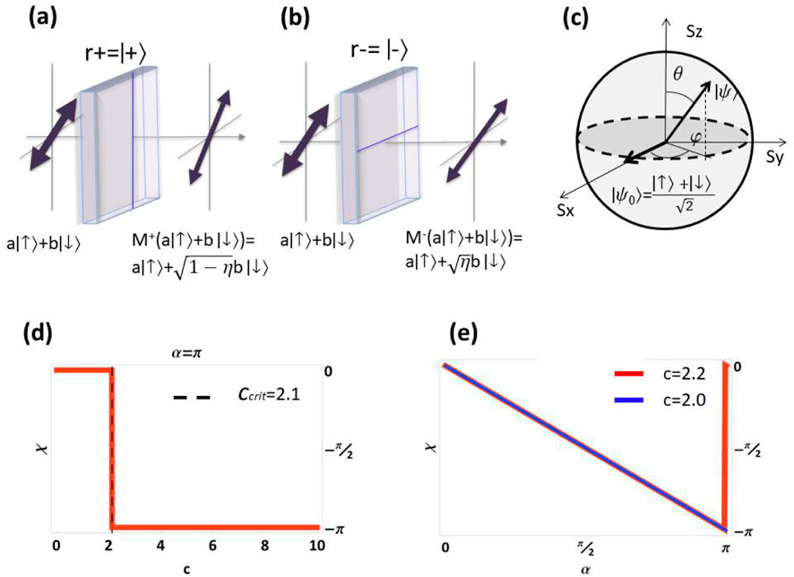
The interaction-induced mapping $(a|\mathbf{n}\rangle +b|-\mathbf{n}\rangle )|+\rangle \to (a|\mathbf{n}\rangle +b\sqrt{1-\eta }|-\mathbf{n}\rangle )|+\rangle +b\sqrt{\eta }|-\mathbf{n}\rangle |-\rangle$ describes the system-detector interaction that mediates the measurement process. The detector is then projectively measured in the basis of states $|\pm \rangle$ after this step. The following properties apply to this measurement protocol: (I) it guarantees that the readout $r=+$ is produced if the initial state is $|\mathbf{n}\rangle$ $(a=1,b=0)$; (II) without changing the system’s state, if the initial state is $|-\mathbf{n}\rangle$ $(a=0,b=1)$, it provides readouts $r=-$ or $r=+$ with probabilities $p_{-}=\eta$ and $p_{+}=1-\eta$, respectively. The measurement procedure does, in fact, change the state of the system when it is in a superposition state of $|\mathbf{n}\rangle$ and $|-\mathbf{n}\rangle$. With probability $\eta |b{|}^2$, the readout results $r=-$, causing a jump in the system state to $|-\mathbf{n}\rangle$. For $\eta \ll 1$, the detector stays essentially in its initial state $(r=+)$, changing the system state only slightly. One can define “null weak values” by taking into account only the experimental runs that result in $r=+$. A photon of a given polarization is always transmitted $(r=+)$, whereas a photon of the orthogonal polarization has a finite probability of being transmitted $(r=+)$ or absorbed $(r=-)$ [2]. Such postselected measurements may be implemented for arbitrary $\eta$ with imperfect polarizers, as shown in Figures 1a, b.

Figure 1

Figure 1. Schematic representation of the action of the measurement protocol described by the proposed POVM set for a generic input state $a|\uparrow \rangle +b|\downarrow \rangle$. Kraus operators $M_{\eta }(\mathbf{n},+/-)$ can be implemented by means of imperfect polarizers oriented along (a) vertical direction $r^{+}=|+\rangle$; (b) horizontal directions $r^{-}=|-\rangle$; (c) depicts the Bloch sphere for the system qubit $\{|\uparrow \rangle ,|\downarrow \rangle \}$ setting the initial state $|{\psi }_0\rangle =\frac{|\uparrow \rangle +|\downarrow \rangle }{\sqrt{2}}$, for initial parameters $({\theta }_0=\pi /2,{\phi }_0=0)$; (d) red curve depicts the $|\pi |$ discrete jump in the geometric phase $(X)$ from 0 to $-\pi$ for a critical measurement strength $c_{\text{crit}}=2.1$ (dashed line indicating the onset of topological phase transition); (e) depicts the topological phase transition in the geometric phase $(X)$ for $\alpha =\pi$, corresponding to a single winding $(W=1)$. Special attention was taken to ensure the continuity of the geometric phase $(X)$ at the point of the phase transition in order to distinguish transitions from random phase jumps.

Within this framework, the weak measurement-induced geometric phase $(X)$ can be defined as $X=\mathrm{a}\mathrm{r}\mathrm{g}\langle {\psi }_0|M_N^{(r_N)}\dots M_1^{(r_1)}|{\psi }_0\rangle$. It can be obtained from the quasi-continuous trajectory with all outcomes set to $r_k=+$, setting the measurements orientations to $({\theta }_k,{\phi }_k=\theta ,2\pi k/N)$, and using the explicit form of the Kraus operators (Equation 2). In particular, for an initial state of the form $|{\psi }_0\rangle =R{({\mathbf{n}}_0)}^{-1}|\uparrow \rangle$, it is possible to rewrite the geometric phase using $\langle {\psi }_0|M_N^{(+)}\dots M_1^{(+)}|{\psi }_0\rangle =\langle \uparrow |\delta R{(M_{\eta }(z,+)\delta R)}^{N-1}|\uparrow \rangle$, where $\delta R$ (Equation 4) can be expressed as [2]:

$\delta R=\left(\begin{array}{cc}\hfill {\cos }^2\frac{\theta }{2}+e^{-2\pi i/N}{\sin }^2\frac{\theta }{2}\hfill & \hfill \frac{1}{2}\left(1-e^{-2\pi i/N}\right)\sin \theta \hfill \\ \hfill \frac{1}{2}\left(1-e^{-2\pi i/N}\right)\sin \theta \hfill & \hfill {\sin }^2\frac{\theta }{2}+e^{-2\pi i/N}{\cos }^2\frac{\theta }{2}\hfill \end{array}\right),(4)$

which is a matrix independent of $k$, as explained in detail in the following Section. An imperfect polarizer oriented along the directions $r^{+,-}$ can implement such null-type weak-measurement protocol. This is depicted in Figure 1. Figure 1a describes the action of the POVM $M_{\eta }(\widehat{z},+)$ on a generic input state $|{\psi }_0\rangle =a|\uparrow \rangle +b|\downarrow \rangle$ while Figure 1b describes the action of the POVM $M_{\eta }(\widehat{z},-)$ on the same generic input state. The Bloch sphere for the system qubit $s=\{|\uparrow \rangle ,|\downarrow \rangle \}$ is schematized in Figure 1c.

3 Analytic results

An analytic expression for the geometric phase $X$ can be derived in the quasicontinuous measurement limit $N\to \infty$. $X$ is extracted from the quasicontinuous trajectory postselecting all outcomes $r_k=|+\rangle$ as described in PNAS2020 [2]. This result is obtained by setting the initial state $|{\psi }_0\rangle =R^{-1}({\mathbf{n}}_{\mathbf{0}})|\uparrow \rangle$. In our case, we consider the initial state to be eigenstate of $S_x$, of the form $|{\psi }_0\rangle =\frac{|\uparrow \rangle +|\downarrow \rangle }{\sqrt{2}}$, thus selecting the initial rotation along $\widehat{x}$, this is equivalent to setting the initial parameters $({\theta }_0=\pi /2,{\phi }_0=0)$, as depicted in Figure 1c. We then sequentially rotate the measurement apparatus, in order to increment the angle $\phi$ by a fixed amount $ϵ=2\pi /N$. This parameterization ensures that the trajectory is closed and the geometric phase well defined. By selecting the readouts $r_k=|+\rangle$, setting $\eta =4c/N$, the measurement orientations $({\theta }_k,{\phi }_k)=(\pi /\mathrm{2,2}\pi k/N)$, and using the explicit form of Kraus operators in Equation 2, one obtains an expression for the geometric phase $X$ of the form [2]:

$\mathrm{a}\mathrm{r}\mathrm{g}\langle {\psi }_0|{\mathcal{M}}_{N-1}^{\left(+\right)}\dots {\mathcal{M}}_1^{\left(+\right)}|{\psi }_0\rangle =\mathrm{a}\mathrm{r}\mathrm{g}\langle \uparrow |\delta R{\left(M_{\eta }\left(\widehat{z},+\right)\delta R\right)}^{N-1}|\uparrow \rangle ,(5)$

where $\delta R$ (Equation 6) is given by the $k$-independent matrix:

$\delta R=\left(\begin{array}{cc}\hfill 1/2\left(1+e^{-iϵ}\right)\hfill & \hfill 1/2\left(1-e^{-iϵ}\right)\hfill \\ \hfill 1/2\left(1-e^{-iϵ}\right)\hfill & \hfill 1/2\left(1+e^{-iϵ}\right)\hfill \end{array}\right).(6)$

The quasicontinuous limit $(N\to \infty )$ is obtained by using the exponential approximation ${(1+\mathrm{\Gamma }/N)}^N\approx e^{\mathrm{\Gamma }}$, valid for $N\to \infty$. This approximation is explicitly invoked by expressing the Taylor series of $M_{\eta }(\widehat{z},+)\delta R$, and rewriting $M_{\eta }(\widehat{z},+)\delta R=V(I+\mathrm{\Gamma }/N)V^{-1}$, where $I$ is the $2\times 2$ identity matrix and $V$ is the unitary matrix for the change of basis, obtained by diagonalization of $M_{\eta }(\widehat{z},+)\delta R$. In this scenario, the geometric phase can be extracted from the upper-most diagonal element of the matrix product $V{e}^{\mathrm{\Gamma }}{V}^{-1}$, resulting in:

$X=e^{-i\alpha -c}\left[\cosh \left(\tau \right)+c\sinh \left(\tau \right)/\tau \right],(7)$

where $\tau =\sqrt{c^2-{\alpha }^2}$ and $\alpha =ϵN/2$. We recover the analytic result reported in [2], by setting $z=c$, and $\alpha =\pi$, as expected for $\theta =\pi /2$.Our knowledge of the existence of a critical-measurement parameter where the geometric phase makes a phase transition is based on the previous work reported in Ref. [2]. We do not analyze a continuous set of trajectories that cover the entire parameter space, as we focus on a specific set of trajectories winding along the equator.

We note that our case is complementary to the one analyzed in PNAS2020 [2], where the authors analyze the dependence of the geometric phase on the azymmuthal angle $\theta$ for a single winding of the trajectory with the polar angle $\phi$. Here we report the dependence of the geometric phase on the winding of the trajectory by the steering sequence of weak measurements of increasing angle $\phi$, obtained by increasing the winding number $W$, while fixing $\theta =\pi /2$. We stress that the critical measurement-strength parameter $c_{\text{crit}}$ obtained for different winding numbers $W=\mathrm{1,2,3},\dots ,M$ (with $M\in Z^{+}$) are not predictable to our knowledge.

The onset of a topological phase transition in the geometric phase for a critical measurement strength can be understood by considering two limiting cases: For the case of a series of strong projective measurements $(c\to \infty )$, resulting in the well-known Pancharatnam-Berry phase $\pi (\cos (\theta )-1)$ [24], the polarization is expected to rotate along the equator by an amount $ϵ=2\pi /N$ with each projective measurement, until it returns to its original state, accumulating a geometric phase equal to $|\pi |$ (modulo $2\pi$), while for a series with infinitely weak measurement strength $(c\to 0)$ the polarization should not be affected by the measurement process. Thus, there exists a critical measurement strength $c_{\text{crit}}$ where $X$ makes a discrete jump from 0 to $|\pi |$, signaling the onset of a topological phase transition, here $|\pi |$ corresponds to a full winding of the trajectory. A plot of the geometric phase $X$, given by the analytic expression in Equation 7, is given in Figures 1d, e. Figure 1d depicts the discrete jump of $X$ from 0 to $-\pi$ for a critical measurement strength $c_{\text{crit}}=2.1$ indicating the onset of topological phase transition, while Figure 1e depicts the geometric phase vs. $\alpha$, signaling a topological phase transition for a $\alpha =\pi$, corresponding to a full winding of the trajectory with the polar phase $(W=1)$. Special attention was taken to ensure that the geometric phase is mathematically continuous in order to distinguish the onset of a topological transition, from a random $\pi$-jump in the geometric phase.

3.1 Winding number $(W)$

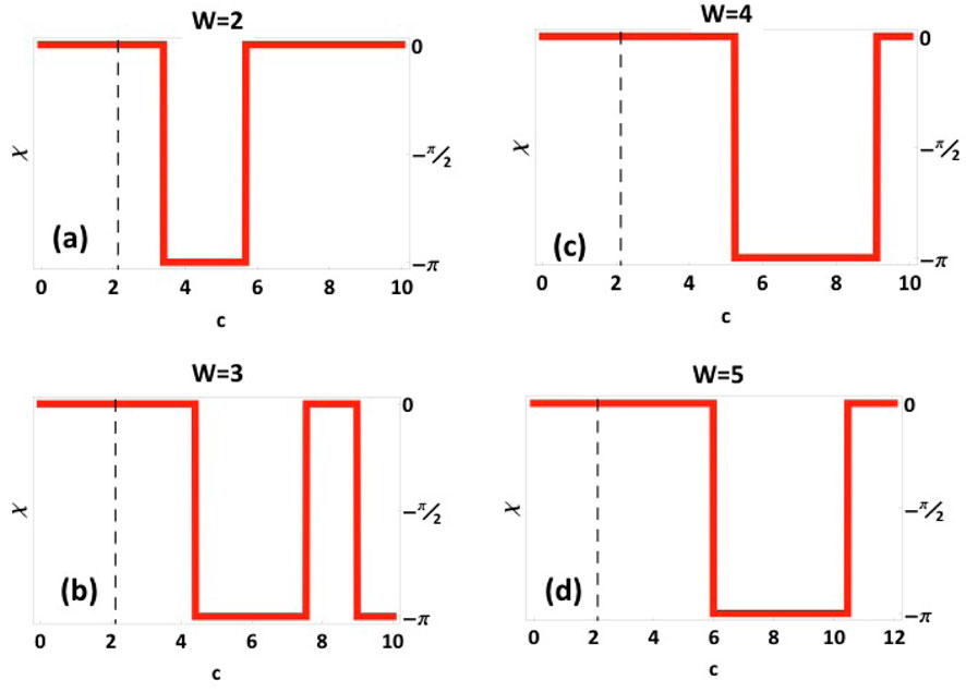
Next, we analyzed the existence of additional critical measurement-strength values, signalling multiple topological phase transitions characterized by discrete jumps in the geometric phase between 0 and $|\pi |$. This was analyzed by enabling the parameter $\alpha$ take multiple values in the intervals $[0,k\pi ]$, with $k=1,\dots ,M$ and $M\in Z^{+}$, corresponding to full windings of the phase $\phi$, as quantified by the winding number $W=k$, with $k=1,\dots ,M$, and a wrapping of the phase at multiples of $2\pi$, revealing the existence of additional critical measurement-strength parameters for different values of $W$. This is shown in Figure 2, displaying additional critical-measurement parameter values where $X$ jumps from $0\to -\pi$ and from $-\pi \to 0$, respectively. We stress that while there is numerical evidence indicating that $c_{\text{crit}}$ increases with $W$, the actual critical measurement-strength values for different winding numbers $W$ are not predictable to our knowledge.

Figure 2

Figure 2. $|\pi |$ discrete jumps in the geometric phase $(X)$ vs. measurement-strength parameter $(c)$ for increased winding number $W=k$, with $k=\mathrm{2,3,4,5}$: (a) $(\alpha =2\pi ,W=2)c_{\text{crit}}=3.4$ and $c_{\text{crit}}=5.7$, (b) $(\alpha =3\pi ,W=3)c_{\text{crit}}=4.4$ and $c_{\text{crit}}=7.6$, (c) $(\alpha =4\pi ,W=4)$ $c_{\text{crit}}=5.2$ and $c_{\text{crit}}=9.1$ and (d) $(\alpha =5\pi ,W=5)c_{\text{crit}}=6.0$ and $c_{\text{crit}}=10.5$. As we restrict our analysis to trajectories on the equator, the acquired geometric phase $(X)$ can only take values of 0 or $|\pi |$ (modulo $2\pi$).

Figure 2 corresponds to: (a) $(\alpha =2\pi ,W=2)$ with $c_{\text{crit}}=3.4$ and 5.7, (b) $(\alpha =3\pi ,W=3)$ with $c_{\text{crit}}=4.4$ and 7.6, (c) $(\alpha =4\pi ,W=4)$ with $c_{\text{crit}}=5.2$ and 9.1 and (d) $(\alpha =5\pi ,W=5)$ with $c_{\text{crit}}=6.0$ and 10.5. We note that as we restrict our analysis to trajectories on the equator, the acquired geometric phase can only take values of 0 or $|\pi |$ (modulo $2\pi$).

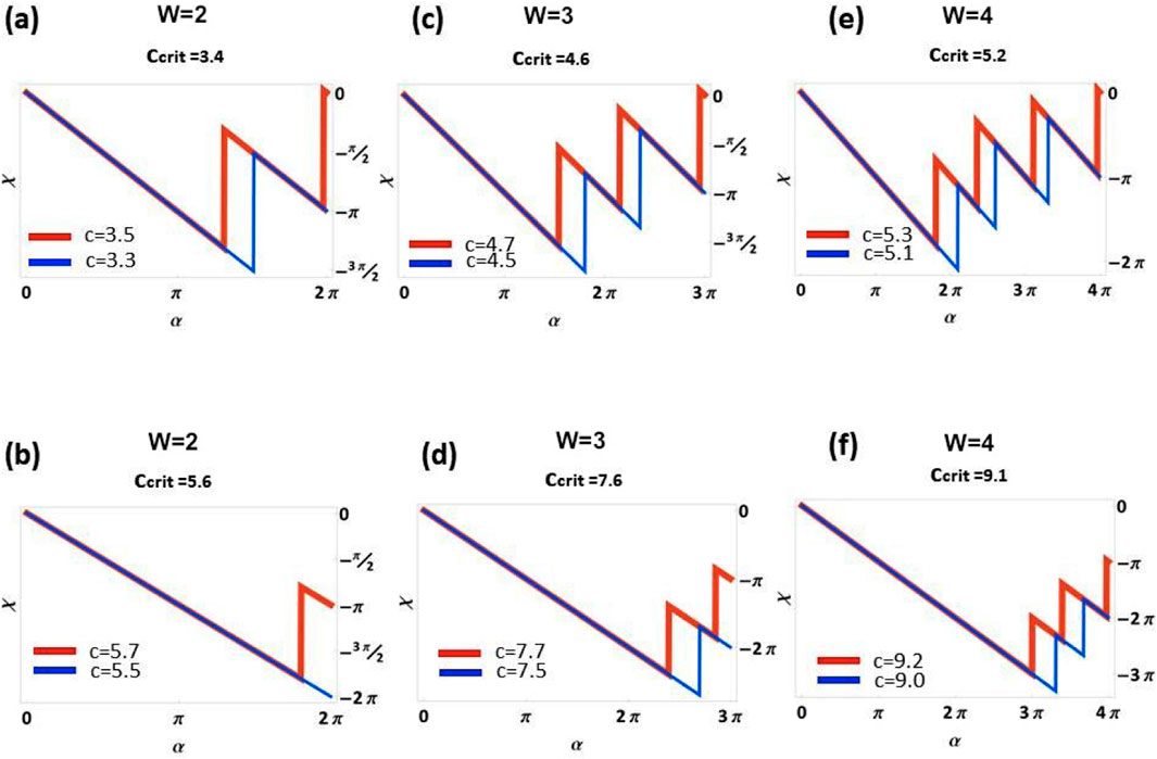
Further confirmation of the onset of different topological phase transition was obtained by plotting the geometric phase vs. the angle parameter $\alpha$ for increased winding number $W$. This is presented in Figure 3, for trajectories with $c<c_{\text{crit}}$ (red curves) and for trajectories with $c>c_{\text{crit}}$ (blue curves). Figures 3a, b depicts curves for $W=2$, and phase transition from 0 to $|\pi |$ and $|\pi |$ to 0 (mod $2\pi$), respectively; (c) and (d) depicts curves for $W=3$, and phase transition from 0 to $|\pi |$ and $|\pi |$ to 0 (mod $2\pi$), respectively; (e) and (f) depicts curves for $W=4$, and phase transition from 0 to $|\pi |$ and $|\pi |$ to 0 (mod $2\pi$), respectively. The different topological nature of each phase transition is signalled by the increased numbers of oscillations for increased $W$. This can be explained by noting that increasing the winding number $W=k$, for $\alpha \in [0,k\pi ]$, corresponds to closing the trajectory after $k$-windings of $2\pi$ of the polar angle $\phi$. Therefore, it is expected to observe a larger number of oscillations for increased windings $W$, as displayed in Figure 3. Figures 3a, c, e display $k$ oscillations for $W=k$, while Figures 3b, d, f present $k-1$ oscillations for $W=k$, since there is no phase transition from $|\pi |$ to 0 (modulo 2$\pi$) for a single winding $W=1$.

The linear dependence of the total acquired phase vs. $\alpha$ is ascribed to the global dynamical term $e^{-i\alpha }$ in Equation 7, resulting in a linear dependence on $\alpha$ for the geometric phase, when plotting its argument. As it was readily predicted in [30], for closed steered trajectories the underlying phase factors involve both dynamical and geometrical terms. Such dynamical phase components can explain deviations in the total acquired phase from the discrete values of 0 or $|\pi |$. A plot of the geometric phase excluding dynamical terms is presented in Supplementary Appendix A.

Our case is analogous to Ref. [2], only restricting our analysis to trajectories winding along the equator of the Bloch sphere $(\theta =\pi /2)$, while focusing our attention on the impact of the winding number $(W)$ on the dynamics of the system. In this scenario, the only possible values $X$ can take, as a consequence of the area subtended by a closed trajectory returning to its initially state are: $X=0$ for an incomplete winding and an open trajectory, or $X=\pi$ (modulo $|2\pi |$) for a full winding and a closed trajectory. The difference in the trajectory on the Bloch sphere for $c>c_{\text{crit}}$ or $c<c_{\text{crit}}$ is given by the corresponding values of $\alpha$ where the full winding takes place, implying an acquired geometric phase $X=\pi$ (modulo $|2\pi |$).

Figure 3

Figure 3. Topological phase transition for increased winding numbers $W=\mathrm{2,3,4}$, for $c>c_{\text{crit}}$ $(c<c_{\text{crit}})$ red (blue) curves: (a, b) depicts curves for $W=2$, and phase transition from 0 to $|\pi |$ and $|\pi |$ to 0, respectively; (c, d) depicts curves for $W=3$, and phase transition from 0 to $|\pi |$ and $|\pi |$ to 0, respectively; (e, f) depicts curves for $W=4$, and phase transition from 0 to $|\pi |$ and $|\pi |$ to 0, respectively. The different topological nature of each phase transition is signalled by the increased numbers of oscillations for increased $W$. This can be explained by noting that increasing the winding number $W=k$, for $\alpha \in [0,k\pi ]$, corresponds to closing the trajectory after $k$-windings of $2\pi$ with the polar angle $\phi$. Therefore, it is expected to observe a larger number of oscillations when increasing the number of windings $W$. (a, c, e) display $k$ oscillations for $W=k$, while (b, d, f) present $k-1$ oscillations for $W=k$, since there is no phase transition from $|\pi |$ to 0 for a single winding $W=1$. Special attention was taken to ensure the continuity of the geometric phase at the point of the phase transition in order to distinguish transitions from random phase jumps.

4 Numerical results

4.1 Quantization of the geometric phase for finite-$N$

The topological character of the phase transition exhibited at the critical measurement-strength parameter $(c_{\text{crit}})$, where the geometric phase $(X)$ makes a $|\pi |$ discrete jump, is clearly revealed by the quantization of $X$ between 0 and $|\pi |$ (modulo $2\pi$). This quantization can be understood as a signature of the so-called “topological protection” of the phase, which prevents fluctuations in the discrete values of the phase acquired by the system under weak perturbations in the protocol. This quantization of the phase, confirming the topological nature of the transition, is clearly valid in the quasicontinuous limit $(N\to \infty )$, where the analytic result holds.

In this Section, we analyze the robustness of the quantization of $X$, with respect to fluctuations in the total number of measurements $N$, meaning that we derive a numerical expression for the geometric phase for finite-$N$. Evidently, this analysis cannot be derived from the analytical result reported in Equation 7, which is only valid for $N\to \infty$ and $N\gg \mathrm{\Gamma }$, for the exponential approximation ${(1+\mathrm{\Gamma }/N)}^N\approx e^{\mathrm{\Gamma }}$ to hold. In order to obtain a numerical value for $X$ and analyze its robustness to different type of noise and perturbations, we follow Equation 5 to obtain a numerical expression for the $N$-matrix product $\delta R{(M_{\eta }(\widehat{z},+)\delta R)}^{N-1}$. Next, we plot the left upper-most matrix element for different values of $N$ and $c$. For $N$ sufficiently large $(N>500)$ and the measurement-strength parameter sufficiently small $(c\ll N)$, the analytic result and numerical results are indistinguishable. We are interested in understanding at which point the numerical result departs from the analytic prediction.

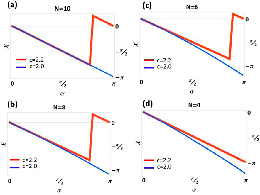
Plots of the geometric phase $X$ vs. $\alpha$ for decreasing values of $N$ are presented in Figure 4, for a measurement-strength parameter $c>c_{\text{crit}}$ (red curves) and $c<c_{\text{crit}}$ (blue curves), where $c_{\text{crit}}\approx 2.1$ for $W=1$. For simplicity, we consider a single winding of the trajectory with the polar angle $W=1$, although the same framework can be applied to $W>1$. Figures 4a–d correspond to $N=\mathrm{10,8,6,4}$, respectively. We note that the deviation of the numerical result from the analytic prediction is readily apparent for $N=8$, where the quantization of $X$ between 0 and $\pi$ vanishes, signaling that the topological nature of the phase transition vanishes. Furthermore, for $N<5$ the discrete jumps in the geometric phase at the critical measurement strength are completely washed out. Our numerical findings confirms that the quantization of $(X)$ not only depends on the measurement strength $c$, but also on the total number of measurements $N$ and its interplay with the $c$-parameter, with fully topological character only for $N>4$, when considering $c_{\text{crit}}=2.1$ $(W=1)$.

Figure 4

Figure 4. Plots of the geometric phase $X$ vs. $\alpha$ for decreasing values of $N$, for a measurement-strength parameter $c>c_{\text{crit}}$ (red curves) and $c<c_{\text{crit}}$ (blue curves), where $c_{\text{crit}}\approx 2.1$ for $W=1$. (a–d) correspond to $N=\mathrm{10,8,6,4}$, respectively. The deviation of the numerical result from the analytic prediction is readily apparent for $N=8$. For $N=4$ the discrete jump in $X$ is fully vanished.

4.2 $N-c$ landscape

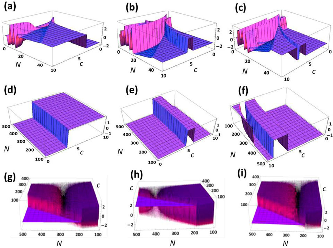
In order to analyze the interplay between the quantization of the geometric phase $X$, for different values of total number of measurements $N$ and strength parameter $c$, we numerically calculated $X$ in different relevant regions of the $N-c$ landscape. This is displayed in the 3D density plot depicted in Figure 5. Figures 5a–c correspond to parameter values of $0<N<50$ and $0<c<10$, for $W=\mathrm{1,2,3}$ respectively. Clearly, in the magenta regions of the 3D plots, it is observed that the stability of the geometric phase is dramatically reduced for $N<20$, meaning that fluctuations in the geometric phase are readily apparent for $N$ of the same order as $c$ $(N\approx c)$. This numerical finding also sets a limit in the actual values of measurement strength $c$ that can be accepted in the quasicontinuous limit. Figures 5d–f present numerical simulations of $X$ considering $100<N<500$ and $0<c<10$, for $W=\mathrm{1,2,3}$ respectively. We find that for $N>100$, corresponding to $N\gg c$, the fluctuations in the geometric phase vanish, meaning that in this region of the $N-c$ landscape the analytic result is fully valid, as reported in [2]. Fluctuations are expected to resurge as $c$ approaches values of the same order of $N$ $(N\approx c)$ [30], or for values larger than $N$ $(N<c)$. This is analyzed in detail in Figures 5g–i, for $100<N<500$ and $100<c<400$, for $W=\mathrm{1,2,3}$, respectively. We note that there is no clear critical measurement-strength parameter in this region where $X$ makes a discrete jump. Nevertheless, it is observed that fluctuations in $X$ arise for $c>300$, for any value of $N$, meaning that the region of validity of the analytical result can only be considered if $N\gg c$, in other words $N>c$ is not acceptable for the analytic result to hold. Evidently, there is no value of $N$ where the analytic result holds for $c>300$. This upperlimit is relevant when analyzing the strong-measurement limit $c\to \infty$, as considered in Snizhko et al. [30], and for feasible experimental realizations of the scheme [31, 32].

Figure 5

Figure 5. 3D plots of the geometric phase $X$ for different regions of the $N-c$ landscape. Such regions correspond to parameter values $N\gg c$, $N\approx c$, and $N\ll c$. For $N\gg c$ it is observed a constant geometric phase $X$, with discrete jumps of $|\pi |$ at the critical measurement-strength parameter $c_{\text{crit}}$, as predicted by the analytical result. For $N\approx c$, we observe slow oscillatory behaviour in the geometric phase $X$, anticipating the regions of parameter space for $N\ll c$, where we observe fast oscillatory response in the geometric phase $X$, corresponding to parameter regions where the Kraus operator $M_{\eta }(+)$ becomes imaginary $(4c/N>1)$. (a–c) correspond to parameter values of $0<N<50$ and $0<c<10$, for $W=\mathrm{1,2,3}$ respectively. (d–f) present numerical simulations of $X$ considering $100<N<500$ and $0<c<10$, for $W=\mathrm{1,2,3}$ respectively. The magenta appearance of the 3D density plots indicate regions where the stability of the geometric phase is dramatically reduced. (g–i), for $100<N<500$ and $100<c<400$, for $W=\mathrm{1,2,3}$, respectively. It is observed that fluctuations in $X$ arise for $c>300$, for any value of $N$. Moreover, in the stable region characterized by $N\gg c$, there is no apparent critical measurement-strength parameter where $X$ makes a discrete jump.

The resolution considered in Figure 5 corresponds to $\mathrm{\Delta }N=1,\mathrm{\Delta }c=0.01$ in (a)-(f) and $\mathrm{\Delta }N=1,\mathrm{\Delta }c=0.5$ for the fast oscillations in (g)-(i). In addition, we performed an extensive analysis of the impact of resolution on the slow and fast oscillations in Figure 5 in order to confirm they are of physical origin and not a numerical artefact. A detailed discussion on the resolution considered in the numerical simulations is presented in Supplementary Appendix B.We note, the Kraus operator $M_{\eta }(\widehat{z},+)$ in Equation 2 should be real in order to correspond to a measurement-induced polarization rotation, as required in order to steer the trajectory. This, in turn, requires $0\le \eta \le 1$. For $\eta >1$, $M_{\eta }(\widehat{z},+)$ becomes imaginary, thus corresponding to a phase retardation. This further explains the observed deviations of the numerical results from the analytic prediction in Figures 4, 5. In order to ensure $0\le \eta \le 1$, it is possible to define an effective measurement-strength parameter ${\eta }_{\mathrm{e}\mathrm{ff}}=1-e^{-4c}$, which is independent of $N$ and can be used to analyze the strong-measurement limit $(c\to \infty )$, where one obtains Zeno-like dynamics: The state follows meticulously the measurement orientation, and the geometric phase becomes the Pancharatnam-Berry phase [2]. Nevertheless, in this work we are not interested in such limit, as we want to uncover the point at which the numerical results deviate from the analytic prediction.

4.3 Phase noise

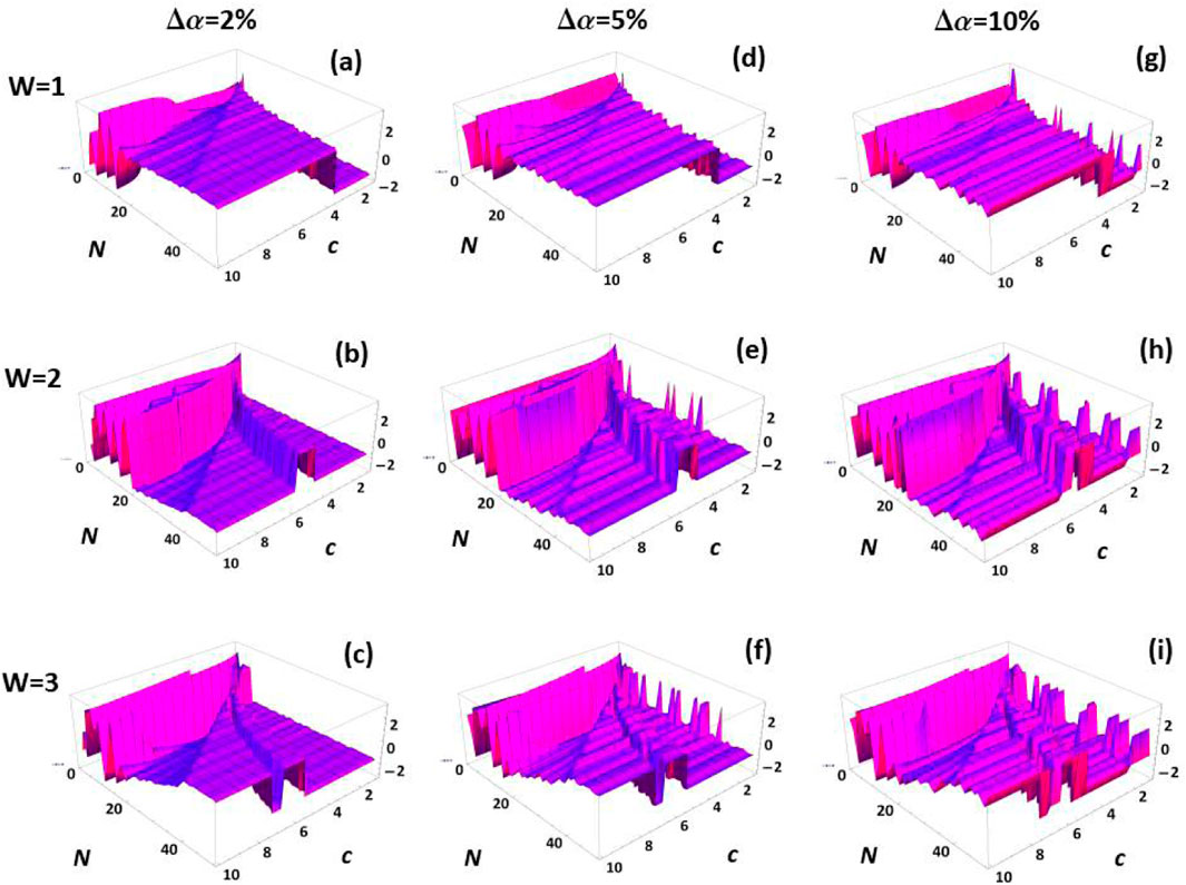
In order to characterize the robustness of the measurement protocol to experimental errors arising as a result of phase fluctuations due to limited temporal stability of the system, which can result, for example, as a consequence of temperature, spatial, frequency, or polarizations drifts, among other realistic sources of errors. We analyze the effect of uncorrelated phase noise on the geometric phase $X$ in the $N-c$ landscape, although other forms of correlated noise could be considered, for instance noise linearly or polynomially correlated with the total number of measurements $N$, and the measurement strength $c$. We model the phase noise $\mathrm{\Delta }\alpha$ with a normal distribution centred around ${\alpha }_0=\pi$, with varying spreads $\mathrm{\Delta }\alpha =2\%,5\%,10\%$, considering different winding numbers for the polar angle $W=\mathrm{1,2,3}$. Plots of the accumulated phase noise for different regions of the $N-c$ landscape are presented in Figures 6–8. Numerical simulations of uncorrelated phase noise in the region $0<N<50$ and $0<c<10$ are presented in Figure 6. Figures 6a–c correspond to phase noise with a spread $\mathrm{\Delta }\alpha =2\%$ for $W=\mathrm{1,2,3}$, respectively. Figures 6d–f correspond to phase noise with a spread $\mathrm{\Delta }\alpha =5\%$ for $W=\mathrm{1,2,3}$, respectively. Figures 6g–i correspond to phase noise with a spread $\mathrm{\Delta }\alpha =10\%$ for $W=\mathrm{1,2,3}$, respectively. Clearly, for $\mathrm{\Delta }\alpha >2\%$ fluctuations in the phase render the measurement protocol significantly unstable, and the topological quantization of the phase between 0 and $\pi$ is blurred.

Figure 6

Figure 6. Numerical simulations of uncorrelated phase noise in the parameter region $0<N<50$ and $0<c<10$ of the $N-c$ landscape. (a–c) correspond to phase noise with a spread $\mathrm{\Delta }\alpha =2\%$ for $W=\mathrm{1,2,3}$, respectively; (d–f) correspond to phase noise with a spread $\mathrm{\Delta }\alpha =5\%$ for $W=\mathrm{1,2,3}$, respectively; (g–i) correspond to phase noise with a spread $\mathrm{\Delta }\alpha =10\%$ for $W=\mathrm{1,2,3}$, respectively. For $\mathrm{\Delta }\alpha >2\%$ fluctuations in the phase render the measurement protocol significantly unstable.

Figure 7

Figure 7. Numerical simulations of uncorrelated phase noise in the parameter region $100<N<500$ and $0<c<10$ of the $N-c$ landscape. (a–c) correspond to phase noise with a spread $\mathrm{\Delta }\alpha =2\%$ for $W=\mathrm{1,2,3}$, respectively; (d–f) correspond to phase noise with a spread $\mathrm{\Delta }\alpha =5\%$ for $W=\mathrm{1,2,3}$, respectively; (g–i) correspond to phase noise with a spread $\mathrm{\Delta }\alpha =10\%$ for $W=\mathrm{1,2,3}$, respectively. This region of the $N-c$ landscape is significantly robust to uncorrelated phase noise and the quantization of the phase is typically preserved.

Figure 8

Figure 8. Numerical simulations of uncorrelated phase noise in the parameter region $100<N<500$ and $100<c<400$ of the $N-c$ landscape. (a–c) correspond to phase noise with a spread $\mathrm{\Delta }\alpha =2\%$ for $W=\mathrm{1,2,3}$, respectively; (d–f) correspond to phase noise with a spread $\mathrm{\Delta }\alpha =5\%$ for $W=\mathrm{1,2,3}$, respectively; (g–i) correspond to phase noise with a spread $\mathrm{\Delta }\alpha =10\%$ for $W=\mathrm{1,2,3}$, respectively. In this limit, the only region of the $N-c$ landscape robust to phase noise if for $N\gg c$ and $c<300$.

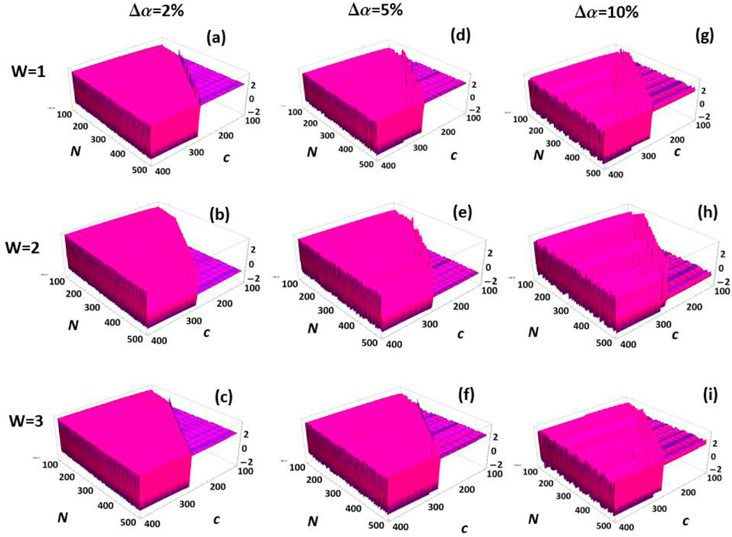
Next, numerical simulations of uncorrelated phase noise in the region $100<N<500$ and $0<c<10$ are presented in Figure 7. Figures 7a–c correspond to phase noise with a spread $\mathrm{\Delta }\alpha =2\%$ for $W=\mathrm{1,2,3}$, respectively. Figures 7d–f correspond to phase noise with a spread $\mathrm{\Delta }\alpha =5\%$ for $W=\mathrm{1,2,3}$, respectively. Figures 7g–i correspond to phase noise with a spread $\mathrm{\Delta }\alpha =10\%$ for $W=\mathrm{1,2,3}$, respectively. Clearly, this region of the $N-c$ landscape is significantly robust to uncorrelated phase noise, and the (topological) quantization of the phase is preserved.

Finally, numerical simulations of uncorrelated phase noise in the region $100<N<500$ and $100<c<400$ are presented in Figure 8. Figures 8a–c correspond to phase noise with a spread $\mathrm{\Delta }\alpha =2\%$ for $W=\mathrm{1,2,3}$, respectively. Figures 8d–f correspond to phase noise with a spread $\mathrm{\Delta }\alpha =5\%$ for $W=\mathrm{1,2,3}$, respectively. Figures 8g–i correspond to phase noise with a spread $\mathrm{\Delta }\alpha =10\%$ for $W=\mathrm{1,2,3}$, respectively. Clearly, in this limit the only region of the $N-c$ landscape robust to phase noise if for $N\gg c$ and $c<300$, we note that there is no clear critical measurement-strength parameter $c$ in this region where $X$ makes a discrete jump. Numerical results considering phase noise confirm the findings in Figure 5, with the additional insight that the $N-c$ landscape region $0<N<50$ and $0<c<10$ is not sufficiently robust to phase noise $\mathrm{\Delta }\alpha >2\%$. Thus the only entirely acceptable region, regarding uncorrelated phase noise, is for $N\gg c$ and $c<300$, such as the case considered in Figure 7, and in PNAS2020 [2].

5 Discussion

We presented an analytical and numerical study of a novel type of geometric phase induced by weak measurements. In contrast to the case considered by Gebhart et al. [2], the originality of our approach consists of considering the dependence of the geometric phase on the winding $W$ of the trajectory with the polar angle $\phi$, quantifying the number of full $2\pi$-turns the trajectory makes until it closes its path, enabling to define a geometric phase $X$. This is accomplished by fixing the azymmuthal angle at $\theta =\pi /2$ for a sequence of weak measurements in the angle $\phi$ of increasing magnitude ${\phi }_k=ϵk$, with $k=1,,N$ the measurement index. We ensure the trajectory induced by the sequence of weak measurements is closed, and the geometric phase well defined, by parameterizing the rotation parameter as $\alpha =ϵN/2$, where $N$ is the number of measurements. We find that different winding numbers $W$ can give rise to unpredictable critical measurement-strength parameters, where the geometric phase makes a $|\pi |$ discrete jump and the system undergoes a topological phase transition. Furthermore, adding to the novelty of our approach, we not only analyze the weak-measurement induced geometric phase by a full analytic derivation based on the exponential approximation proposed in [2], valid for $N\to \infty$, but also we analyze the induced geometric phase numerically, thus enabling us to understand the finite-$N$ interplay of $X$ with the measurement-strength parameter $c$, and its stability to fluctuations in the protocol.

In particular, we analyzed the impact of uncorrelated phase noise on the quantization of the geometric phase. We find that while the parameter region $N\gg c$ of the $N-c$ landscape, characterized by parameter values $100<N<500$ and $0<c<10$, is significantly robust to phase noise up to $\mathrm{\Delta }\alpha \le 10\%$, the parameter region $0<N<50$ and $0<c<10$ can only support phase fluctuations within $\mathrm{\Delta }\alpha <2\%$. For $c$ of the same order as $N$ $(N\approx c)$, or $c>300$, we find no critical measurement-strength parameter where the geometric phase makes a $|\pi |$ discrete jump. Other models for correlated noise, for instance phase noise increasing with the number of measurements $N$ and/or with the measurement-strength parameter $c$ will be considered in a forthcoming work.

We argue that the exhibited sharp transition in the acquired geometric phase indicates that our protocol could find relevant applications in measurement-induced manipulation and control of quantum states, for instance via the implementation of polarization switches or control-NOT gates, among other potential methods for quantum information processing. More specific, by tuning the coupling parameter $\eta$, for instance by increasing or decreasing the integration time $T$, which determines the level of coupling between the detection qubit and the system qubit, it is possible to trigger a sharp transition in the geometric phase, which can be used as a quantum switch to manipulate and control quantum systems, with high precision. Our findings also have repercussions on the understanding of the foundations of quantum mechanics and quantum measurement theory itself [33].

Data availability statement

The data supporting the conclusions of this article will be made available by the author upon request.

Author contributions

GP: Conceptualization, Formal Analysis, Investigation, Methodology, Resources, Software, Validation, Visualization, Writing – original draft, Writing – review and editing.

Funding

The author(s) declare that financial support was received for the research and/or publication of this article. GP acknowledges financial support from PICT2015-0710 grant and Raices Programme.

Acknowledgments

The author is grateful to Yuval Gefen, Kyrylo Snizhko, and Alessandro Romito, for many insightful discussions, and significant assistance in the development of the numerical codes.

Conflict of interest

The author declares that the research was conducted in the absence of any commercial or financial relationships that could be construed as a potential conflict of interest.

Generative AI statement

The author(s) declare that no Generative AI was used in the creation of this manuscript.

Publisher’s note

All claims expressed in this article are solely those of the authors and do not necessarily represent those of their affiliated organizations, or those of the publisher, the editors and the reviewers. Any product that may be evaluated in this article, or claim that may be made by its manufacturer, is not guaranteed or endorsed by the publisher.

Supplementary Material

The Supplementary Material for this article can be found online at: https://www.frontiersin.org/articles/10.3389/fphy.2025.1562928/full#supplementary-material

References

1. Messiah A. Quantum mechanics. Dover Publications (1961).

Google Scholar

2. Gebhart V, Snizhko K, Wellens T, Buchleitner A, Romito A, Gefen Y. Topological transition in measurement-induced geometric phases. Proc Nat Acad Sci (2020) 117:5706–13. doi:10.1073/pnas.1911620117

PubMed Abstract | CrossRef Full Text | Google Scholar

3. Berry MV. Quantal phase factors accompanying adiabatic changes. Proc R Soc. Lond A (1984) 392:45–57. doi:10.1098/rspa.1984.0023

CrossRef Full Text | Google Scholar

4. Zhang Y, Tan Y-W, Stormer HL, Kim P. Experimental observation of the quantum Hall effect and Berry’s phase in graphene. Nature (2005) 438:201–4. doi:10.1038/nature04235

PubMed Abstract | CrossRef Full Text | Google Scholar

5. Kane CL, Mele EJ. Topological order and the quantum spin Hall effect. Phys Rev Lett (2005) 95:146802. doi:10.1103/physrevlett.95.146802

PubMed Abstract | CrossRef Full Text | Google Scholar

6. Delacretaz G, Grant E, Whetten R, Wöste L, Zwanzinger J. Phys Rev Lett (1986) 56:259. doi:10.1103/PhysRevLett.56.2598

PubMed Abstract | CrossRef Full Text | Google Scholar

7. Xiao D, Chang MC, Niu Q. Berry phase effects on electronic properties. Rev Mod Phys (2010) 82:1959–2007. doi:10.1103/revmodphys.82.1959

CrossRef Full Text | Google Scholar

8. Zhu S-L, Zanardi P. Geometric quantum gates that are robust against stochastic control errors. Phys Rev A (2005) 72:020301. doi:10.1103/physreva.72.020301

CrossRef Full Text | Google Scholar

9. Aharonov Y, Anandan J. Phase change during a cyclic quantum evolution. Phys Rev Lett (1987) 58:1593–6. doi:10.1103/physrevlett.58.1593

PubMed Abstract | CrossRef Full Text | Google Scholar

10. Samuel J, Bhandari R. General setting for Berry’s phase. Phys Rev Lett (1988) 60:2339–42. doi:10.1103/physrevlett.60.2339

PubMed Abstract | CrossRef Full Text | Google Scholar

11. Wilczek F. Fractional statistics and anyon superconductivity. Singapore: World Scientific Publishing (1990).

CrossRef Full Text | Google Scholar

12. Law KT, Feldman DE, Gefen Y. Electronic Mach-Zehnder interferometer as a tool to probe fractional statistics. Phys Rev B (2006) 74:045319. doi:10.1103/physrevb.74.045319

CrossRef Full Text | Google Scholar

13. Nayak C, Simon SH, Stern A, Freedman M, Das Sarma S. Non-Abelian anyons and topological quantum computation. Rev Mod Phys (2008) 80:1083–159. doi:10.1103/revmodphys.80.1083

CrossRef Full Text | Google Scholar

14. Thouless DJ, Kohmoto M, Nightingale MP, den Nijs M. Quantized Hall con-ductance in a two-dimensional periodic potential. Phys Rev Lett (1982) 49:405–8. doi:10.1103/physrevlett.49.405

CrossRef Full Text | Google Scholar

15. Bernevig BA. Topological insulators and topological superconductors. Princeton University Press (2013).

Google Scholar

16. Asboth JK, Oroszlany L, Palyi A. A short course on topological insulators. Springer International Publishing (2016).

CrossRef Full Text | Google Scholar

17. Atala M, Aidelsburger M, Barreiro J, Abanin D, Kitagawa T, Demler E, et al. Direct measurement of the Zak phase in topological Bloch bands. Nat Phys. (2013) 9:795–800. doi:10.1038/nphys2790

CrossRef Full Text | Google Scholar

18. Longhi S. Zak phase of photons in optical waveguide lattices. Opt Lett (2013) 38:3716. doi:10.1364/ol.38.003716

PubMed Abstract | CrossRef Full Text | Google Scholar

19. Loredo J, Broome M, Smith D, White A. Observation of entanglement-dependent two-particle holonomic phase. Phys Rev Lett (2014) 112:143603. doi:10.1103/physrevlett.112.143603

PubMed Abstract | CrossRef Full Text | Google Scholar

20. Puentes G. Spontaneous parametric down conversion and quantum walk topology. JOSA B (2016) 33:461–3224. doi:10.1364/josab.33.000461

CrossRef Full Text | Google Scholar

21. Puentes G. Topology and holonomy in discrete-time quantum walks. Crystals (2017) 7:122. doi:10.3390/cryst7050122

CrossRef Full Text | Google Scholar

22. Neves L, Puentes G. Photonic discrete-time quantum walks and applications. Entropy (2018) 20:731. doi:10.3390/e20100731

PubMed Abstract | CrossRef Full Text | Google Scholar

23. Puentes G. 2D Zak phase lanscape in photonic discrete-time quantum walks, accepted for publication in quantum rep. arXiv (2023). doi:10.3390/quantum1010000

CrossRef Full Text | Google Scholar

24. Pancharatnam S. Generalized theory of interference, and its applications. Proc Indian Acad Sci Sect A (1956) 44:247–62. doi:10.1007/bf03046050

CrossRef Full Text | Google Scholar

25. Berry MV, Klein S. Geometric phases from stacks of crystal plates. J Mod Optic (1996) 43:165–80. doi:10.1080/09500349608232731

CrossRef Full Text | Google Scholar

26. Facchi P, Klein AG, Pascazio S, Schulman LS. Berry phase from a quantum Zeno effect. Phys Lett A (1999) 257:232–40. doi:10.1016/s0375-9601(99)00323-0

CrossRef Full Text | Google Scholar

27. Murdoch KW, Weber SJ, Macklin C, Siddiqui I. Observing single quantum trajectories of a superconducting quantum bit. Nature (2013) 502:2|1–214. doi:10.1038/nature12539

CrossRef Full Text | Google Scholar

28. Minev ZK, Mundhada S, Shankar S, Reinhold P, Gutiérrez-Jáuregui R, Schoelkopf R, et al. To catch and reverse a quantum jump mid-flight. Nature (2019) 570:200–4. doi:10.1038/s41586-019-1287-z

PubMed Abstract | CrossRef Full Text | Google Scholar

29. Weber SJ, Chantasri A, Dressel J, Jordan AN, Murch KW, Siddiqi I. Mapping the optimal route between two quantum states. Nature (2014) 511:570–3. doi:10.1038/nature13559

PubMed Abstract | CrossRef Full Text | Google Scholar

30. Snizhko K, Rao N, Kumar P, Gefen Y. Weak-measurement-induced phases and dephasing: broken symmetry of the geometric phase. Phys Rev Res (2021) 3:043045. doi:10.1103/physrevresearch.3.043045

CrossRef Full Text | Google Scholar

31. Wang Y, Snizhko K, Romito A, Gefen Y, Murch K. Observing a topological transition in weak-measurement- induced geometric phases. Phys Rev Res (2022) 4:023179. doi:10.1103/physrevresearch.4.023179

CrossRef Full Text | Google Scholar

32. Ferrer-Garcia MF, Snizhko K, D’Errico A, Romito A, Gefen Y, Karimi E. Topological transitions of the generalized Pancharatnam-Berry phase. Sci Adv (2023) 9:1. doi:10.1126/sciadv.adg6810

CrossRef Full Text | Google Scholar

33. Puentes G, Datta A, Feito A, Eisert J, Plenio M, Walmsley I. Entanglement quantification from incomplete measurements: applications using photon-number-resolving weak homodyne detectors. New J Phys (2010) 12:033042. doi:10.1088/1367-2630/12/3/033042

CrossRef Full Text | Google Scholar