Simulation analysis on the evolution driven model of global copper ore trade network

Introduction: In the context of energy transition, the competition for copper resources among countries has intensified, and the global copper trade has become a vitally important trade chain. The global copper ore trade network is influenced by various factors, including resource distribution, supply, demand, prices, transportation costs, etc.

Methods: To understand the evolution process of copper trade network and to predict the trend of supply chain structure evolution in future, in this paper, we construct a spatial weighted complex network evolution model based on complex network theory and gravity model using the import and export data and distance data of countries from 1990 to 2022.

Results and discussion: Simulation results show that the possibility of establishing copper ore trade between countries follows the spatial weighted complex network evolution model. It is proportional to the expected trade flow between countries and inversely proportional to the distance. The model will support the simulation analysis of the supply chain network structure evolution and help to carry out in-depth research on the forecast of future trade relations between important countries.

1 Introduction

In recent years, copper has been widely used in new energy-related industries, such as transmission lines, transformers, cable shielding belts and high-end radiators, which are important support for the construction of renewable energy generation installations (such as wind turbines) and solar photovoltaic panels [1–3]. With the rapid development of clean energy and energy-saving technologies, and the global copper demand will continue to grow in a long term [4–6]. Copper resources are abundant globally, but the distribution is unbalanced among countries, due to the different geological conditions [7]. Major copper exporters include Chile, Peru and the Democratic Republic of Congo, and major importers are concentrated in Asia and Europe, such as China, Japan, Germany, Spain and so on. With the increase of copper demand, the competition for copper resources among countries has intensified, and the global copper trade has become a vitally important trade chain. Therefore, studying the supply chain evolution pattern of copper with different characteristics in international trade helps to study the formation and evolution mechanism of copper trade pattern, and predict the trend of supply chain structure evolution based on future trade demand.

In recent years, the study of mineral resources supply chain and the associated risks have gradually become a current research Frontier and hot spot in the field of resources, which has received attention from global scholars [8–12]. The research object gradually expands from energy minerals such as oil, natural gas to emerging minerals such as lithium, nickel and rare earth involved in new energy and other emerging industries [13–15]. The research mainly focuses on the trade flows among countries, trade structure characteristics of different mineral products in the whole industry chain and risk resistance of supply chain network [16]. Based on the industry chain perspective, many scholars have made a series of research advances by constructing models to research structure, resilience and risk of supply chain by complex network, SD simulation, material flow analysis (MFA/SFA), gravity model, Markov Chain and other simulation models [17–23]. Complex network can systematically describe the structural characteristics of mineral resource supply chains. Many Scholars have established network models based on trade flows, taking countries as nodes [24, 25]. Most of them focus on the description of topological characteristics of trade networks, the analysis of important nodes and the propagation of risks in supply chain networks [26, 27]. Fewer studies have been conducted on the driving models and mechanisms behind the evolution of supply chain network structures. Some research considers the influence of a single factor or multiple factors such as supply, demand, price, economics and others on the global copper trade using the gravity model, but little evidence has been provided to reveal the evolutionary mechanism of the copper trade network structure, especially the role of geographical factors in the evolution processed of network structures.

Therefore, this paper proposes a spatial weighted complex network evolution model that integrates the complex network theory and gravity model to analyze the evolutionary mechanism of network structure in copper trade. Utilizing this model facilitates the simulation and examination of the evolutionary dynamics within the spatially weighted network of the global copper trade. It explains the formation of the current trade network structure and reveals the role that geographical factors play in shaping trade patterns. The import and export data and distance data of countries from 1990 to 2022 are used to simulate the evolution process of the global copper network. The parameters of the model are discussed by comparing the simulated network structure with the real network structure. Based on the model, the trend of supply chain structure and the potential trading countries can be forecasted. The approach is helpful for trading countries to master their own characteristics and development trends of trade structure, and prepare for trade risks in a timely manner to reduce trade risks. The remainder of this paper is organized as follows. Section 2 describes the construction of the spatial weighted complex network evolution model and data sets used in our work. Section 3 presents the results about evolutionary process of the global copper ore trade network. We summarize our conclusions in Section 4.

2 Methods and data

2.1 Complex network model of international trade in copper ore

According to the complex network theory, this paper constructs a weighted directed network model for the international copper ore trade, as shown in Equation 1 [28]:

$\mathrm{G}=\left(\mathrm{N},\mathrm{E},\mathrm{W}\right)(1)$

where N is the node, which is the set of all the countries involved in copper ore trade, E is the edge between two nodes. It represents the trade relationship between two country nodes, and the direction of the edge represents the trade flow between two nodes. If there is a trade relationship between two country nodes, there is a continuous edge between the two nodes; if there is no trade relationship between the two country nodes, there is no continuous edge between the two nodes. W is the weight of the continuous edge, which is the trade volume between the two country nodes.

The digraph G is represented by a matrix ${\phi }_{ij}$ with N rows and N columns. If there is a directed edge between node $i$ and node $j$, and its weight is $\tau$, as shown in Equation 2.

${\phi }_{ij}=\phi \left[i,j\right]=\tau (2)$

The average path length signifies the mean trade distance among countries, with shorter lengths indicating closer and more intimate trade relationships between them [29]. The definition of average short path length(L) is given in Equation 3.

$L=\frac{1}{N\left(N-1\right)}{\displaystyle \sum _{i\ne j}}{d}_{ij}(3)$

where $N$ is the total number of nodes, $d_{ij}$ is the shortest path between the nodes $i$ and $j$.

The average clustering coefficient serves as a metric to quantify the proximity of trading partners in terms of their trade structure [22]. A higher average clustering coefficient implies a tighter relationship, thereby enhancing the likelihood of establishing long-term and stable trade relations among the partners. The definition of the average clustering coefficient of a network is given in Equation 4.

$C=\frac{1}{N}{\displaystyle \sum _{i=1}^N}\frac{n_i}{g_i\left(g_i-1\right)}(4)$

where C represents the average clustering coefficient, $n_i$ is the number of edges between all adjacent nodes of node $i$; $g_i$ is the number of all neighboring nodes of node $i$.

The betweenness centrality of a node is often used to reflect its contribution to network connectivity [30]. It is calculated as the ratio of the number of shortest paths passing through the node to the total number of all shortest paths in the network. The larger the ${BC}_i$, the stronger the intermediary regulation ability, and the stronger the control over the trade network. The definition of the betweenness centrality ($\left.B_i\right)$ of a node is given in Equation 5.

$B_i=\frac{2}{\left(N-1\right)\left(N-2\right)}{\displaystyle \sum _{p=1}^N}{\displaystyle \sum _{q=1}^N}\frac{R_{pq\left(i\right)}}{R_{pq}}(5)$

where $R_{pq}$ is the shortest path between p and q, $R_{pq\left(i\right)}$ indicating that there is the shortest path from p to q through node $i$ ($i\ne p\ne q;$$p=1,2,3,\dots ,N;q=1,2,3,\dots ,N$).

The closeness centrality measures the proximity of a trading country to other countries within a complex network, typically quantified as the reciprocal of the summed shortest paths between that country and all others. The higher the value of closeness centrality C signifies the trading country is more significant and difficult to be controlled by other countries [31]. Closeness centrality ($K_i$) is defined by Equation 6.

$K_i=\frac{1}{{\displaystyle \sum _{j=1}^N}{d}_{ij}}(6)$

The eigenvector centrality uses the importance and influence of neighboring countries to describe the role of the country’s trade in the complex network [30]. These countries display the attribute of “strengthening through collaboration with prominent trade nations,” implying that countries with higher eigenvector centrality are typically interconnected with major trading hubs. This underscores their capacity to exert indirect influence on the trade structure. Eigenvector centrality (${\mu }_i$) is defined by Equations 7, 8.

$HX=\mu X(7)$

${\mu }_i{x}_i=h_{1i}{x}_1+h_{2i}{x}_2+\cdots +h_{Ni}{x}_i(8)$

where H is an $N\times N$ adjacency matrix composed of $h_{ij}$. $h_{ij}$ indicates the importance measure value of node $i$ to $j$. $x=x_1,x_2,\cdots x_N$ indicates the degree centrality of each node. ${\mu }_i$ denotes the eigenvector centrality of node $i$.

2.2 Spatial weighted complex network evolution based on gravity model

Improved gravity models have been widely used to estimate and study inter-city population migration, traffic flow or trade flow [32, 33]. In actual networks such as air and road networks, the influence of geographical factors on the network leads to the “convergence” of network edges [34]. The evolution of the global copper supply chain structure is influenced by a combination of factors such as resource endowments, supply and demand patterns, market prices, geopolitical relationships, regional trade agreements, and transportation costs. The transportation cost can be reflected by the geographical distance between two locations to a certain extent. This paper constructs a spatial weighted complex network model of international trade in copper ore, from the perspective of the dynamics of the evolution of the network structure. The supply-demand relationship and transportation costs of each country node in constructing trade relations have been taken into account. Furthermore, this study has delved into the characteristics of the evolution of the international trade structure for copper ore, along with an examination of the pivotal role played by geographical factors in this evolutionary process.

In this paper, we introduce an improved gravity model as a measure of expected trade flows between nodes, defined by Equation 9.

$F_{ij}=S\frac{{m_i}^{\alpha }{m_j}^{\alpha }}{{r_{ij}}^{\epsilon }}(9)$

where $F_{ij}$ is the expected trade flow between nodes, S is a constant, $m_i$ and $m_j$ represent the degree of adaptation of node i and node j. It is defined as the total export volume of exporting countries and the total import volume of importing countries, representing the trade demand of the country. In general, nodes with larger adaptability often have larger degree values. In this study, the “adaptability” of a node represents the trade demand of a country. A larger value of $m_i$ or $m_j$ indicates a greater trade demand, and thus the node is more likely to establish trade connections, resulting in a larger degree value. $r_{ij}$ is the distance between two countries. Since there are often multiple transportation paths between two countries, it is difficult to obtain actual distance data. Normally, the capital is the economic and trade center of the country, and the distance $r_{ij}$ mainly represents the transportation costs between two countries. So this paper simplifies the transportation distance as a straight-line distance between two national capitals, which is the Euclidean distance between two nodes. Although the actual distance among some countries may be biased, it can roughly reflect the transportation costs in the global iron ore trade. $\alpha$ and $\epsilon$ are two parameters, and their values depend on the network’s ability for nodes to adaptability and dependence on geographical factors. $\alpha$ as the adaptation factor, represents the influence of trade demand on network formation; and $\epsilon$ as the geographical factor, captures the role of distance in trade resistance. It has been proved that in actual networks such as airline networks and urban road networks, $\alpha$ = 1 and $\epsilon$ fluctuates between 0.2 and 2.7 [35–39].

Using the improved gravity model described above, it is possible to predict the trade volume between nodes, describing potential dynamics when the nodes are not yet connected to each other. Since $F_{ij}$ describes only the trade volume generated between node $i$ and node $j$, it does not include those generated by other node pairs that propagate through some non-direct path through the $\left(i,j\right)$ edge.

Based on the above formula the expected trade flow between any two nodes can be calculated. According to the actual network development law, when the cost is limited, investment will be preferentially made in the construction of the areas with the most urgent needs and the largest trade flow demands. Only in this way can the dynamic needs of the network be met, and the expected returns of the network be maximized, as shown in the Equation 10.

$\begin{array}{c}{MaxW}_F={\displaystyle \sum _{i<j}}{F}_{ij}{\phi }_{ij}={\displaystyle \sum _{i<j}}S\frac{{m_i}^{\alpha }{m_j}^{\alpha }}{{r_{ij}}^{\epsilon }}{\phi }_{ij}\\ {\displaystyle \sum _{i<j}}{\phi }_{ij}=\delta \end{array}(10)$

where ${\phi }_{ij}$ is the adjacency matrix of the network, δ is the set number of network edges, and $W_F$ is the total expected trade flow of the network. In building the network, priority is given to connecting those node pairs with larger expected trade flows, starting from the pair of nodes with the largest $F_{ij}$, and connecting the corresponding node pairs in decreasing order of $F_{ij}$ until the simulation network reaches a certain number of edges.

2.3 Data sources

Because the import and export data are collected in different countries, there are some differences in the import and export data reported by countries. For example, the trade volume of China’s exports to Japan comes from China, while the trade volume of Japan’s imports from China comes from Japan. Therefore, the base data used in this paper are from the copper ore import data of UN Comtrade website for the years 1990, 1995, 2000, 2005, 2010, 2015, 2020 and 2021. The copper ore data name is “Copper ores and concentrates,” HS number 2603. Especially the 2021 data is used as the benchmark for the simulation of the supply chain network evolution process. The 2021 data contains a total of 117 countries or regions. Some statistical objects such as “other regions of the world, other regions of Asia” cannot be accurately located to the actual geographical location, so they are excluded in the process of this study. After screening, a total of 114 nodes with 580 connected edges were involved in the modeling and analysis of the network evolution process. For ease of display, the abbreviations of country names are used in the figure.

The data of the distance between countries were obtained from the CEPII database. The CEPII database is a comprehensive multinational database, which contains a large number of trade and globalization related data from various countries and regions around the world. The database is widely used in the field of trade and globalization research and has become a reliable source of theoretical and empirical research for many research institutions, governments and academia worldwide. The geographical distance data between two countries is an indicator provided by the cep database. To facilitate the comparison between models, the trade volume and distance data are normalized in this paper, and the raw data are transformed to the interval [1,10].

3 Modeling and results

3.1 Parametric analysis of global copper ore trade network model

In 2021, the global copper ore trade network contains 114 country nodes with 580 connected edges, including 99 nodes in exporting countries and 72 nodes in importing countries. Through the clustering coefficient C(k)-degree(k) correlation distribution characteristics of the network model (Figure 1), the dependence between the clustering coefficient and degree of the network model can be judged. The clustering coefficient C(k) of the network model decreases with the increase of node degree, so the network is a small-world network. With a small average path length of 2.54 and a small network density of 0.045, it indicates that the countries in this network are loosely connected. An average clustering coefficient value of 0.324 suggests that nodes within the network have a propensity to form densely interconnected clusters, indicating a higher degree of local clustering compared to that observed in random networks [27].

Figure 1

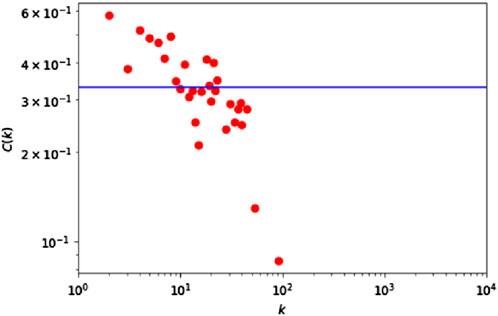
Figure 1. Distribution of model clustering coefficient-degree correlation.

The degree-degree correlation of the network model characterizes the relationship between nodes with large degree and nodes with small degree in the network. If nodes with large degree tend to connect with nodes with large degree, the network exhibits a positive degree-degree correlation feature. Conversely, nodes with large degree tend to connect with nodes with small degree, the network exhibits a negative degree-degree correlation feature. According to the degree-degree correlation distribution of the network model (Figure 2), it can be seen that the nearest neighbor average degree value (knn(k)) of the nodes with degree k is a decreasing function that rises with k. This indicates that the network is a heterogeneous network with negative correlation characteristics, and nodes with large degree tend to connect with nodes with small degree.

Figure 2

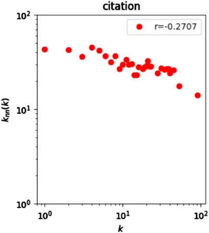
Figure 2. Network model degree - degree correlation distribution.

By constructing the global copper ore trade network model (Figure 3), it can be seen that the countries with larger weighted out degree in the current global trade network include Chile, Peru, Indonesia, Mexico, Australia, etc. They are the main exporting countries of global copper ore. The countries with larger weighted in degree include China, Japan, South Korea, etc., which are the main importing countries of global copper ore.

Figure 3

Figure 3. Global copper supply chain network model (A) weighted out degree, (B) weighted in degree).

By counting the meso-centrality, proximity centrality and eigenvector centrality of each node, the important nodes in the global copper ore trade network are shown in the following table (Table 1). Apart from the major import and export countries, Netherlands, United Arab Emirates, Turkey, United Kingdom and other countries have strong control over the global trade network. Netherlands, Spain and Turkey are also important nodes in the network, they are typically interconnected with major trading hubs.

Table 1

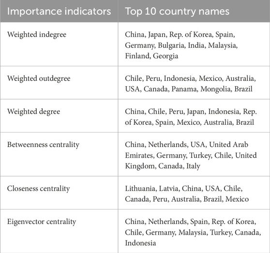
Table 1. Key nodes of the global copper ore trade network.

3.2 Analysis of the historical evolutionary characteristics of the global copper ore trade network

This paper constructs a copper ore supply chain trade network from 1990 to 2021, and analyzes the evolutionary characteristics of the global copper ore trade pattern. From 1990 to 2021, the total volume of global copper ore trade continued to grow, with China’s trade volume gradually dominating the world since 2000 (Figure 4). The total number of countries participating in the global copper ore trade network grew from 43 to 114. The number of trade connecting edges grew from 99 to 580 during the 30-year period. Both the number of nodes and connected edges reached a peak in 2015, then began to decline, and has been growing since 2020 (Figure 5). Combined with the global copper price fluctuations, the changes in the number of nodes and continuous edges are obvious hysteresis to copper price peak.

Figure 4

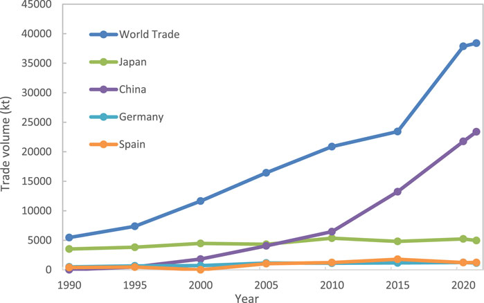
Figure 4. Graph of changes in global and major countries’ copper ore trade volumes (1990-2021).

Figure 5

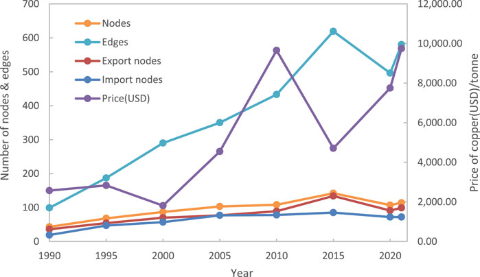
Figure 5. Graph of changes in the size of the global copper ore trading network (1990-2021).

The topological structure characteristics of the network can be judged based on the average degree, average path length, average network density, average clustering coefficient, and degree off the number of ties of the network. The average degree of network, average density of network and average path length are often used to measure the closeness of trade network. The greater the average degree, the greater the density of network, and the smaller the average path length, the more closely connected the network structure is. The average clustering coefficient is used to measure the connectivity of trade between countries, the larger the average clustering coefficient, the better the trade connectivity between countries.

The average degree of the global copper ore trade network has gradually increased over time, with the average path length between any two countries in the network ranging from 2.5 to 3. Since 1995, there has been an overall decreasing trend, indicating that the network tightness has been gradually increasing since 1995. In terms of the change in the average network density, it is highest in 1990, decreasing between 1990 and 2005, increasing from 2005 to 2010, decreasing from 2010 to 2015, reaching a minimum in 2015, and increasing after 2015. This may due to the fact that the network in 1990 contained fewer nodes and the network size was smaller, thus having a smaller average path length and a larger network density. the growth rates of the number of nodes from 1990 to 2020 were 58%, 28%, 18%, 4%, 31%, 25%, and 7%, respectively. The number of nodes increased significantly from 1990 to 2005 and 2015, the network size increased rapidly, and the average density of the network has decreased (Figure 6). Overall, the global copper ore trade network is gradually expanding, and the degree of network tightness is affected by the expansion rate. So, more low-degree nodes entering the network during the rapid expansion phase, resulting in a decrease in the average network density. There is an increase in network tightness during the slow expansion phase through the establishment of more connections between nodes.

Figure 6

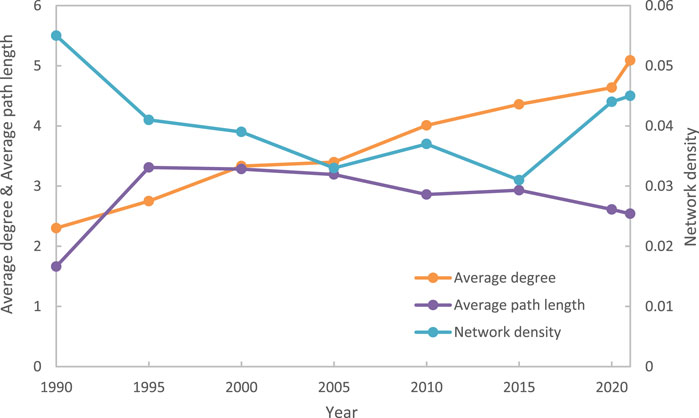
Figure 6. Characterization of the topology of the global copper ore trade network (1990-2021).

The average clustering coefficient of the network keeps increasing, the small-world characteristic tends to be obvious (Figure 7). The trade connectivity among countries becomes stronger. Combined with the clustering coefficient-degree correlation distribution (Figure 8), it can be seen that the change of clustering coefficient with node degree is not obvious before 2010, and after 2010. The clustering coefficient decreases with the increase of node degree, and the network shows the typical power-law distribution characteristics. There are hub nodes in the network, and the hub nodes make the distance between each other shorter by connecting a large number of low-degree nodes. It greatly shortens the path length and strengthens the connectivity of the network.

Figure 7

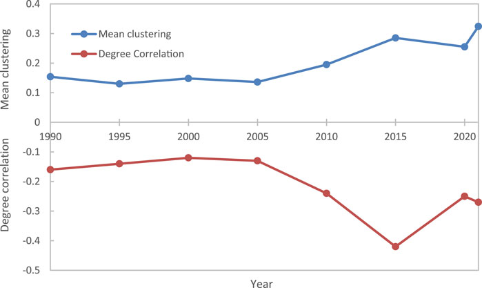
Figure 7. Graph of the change in clustering coefficient and degree correlation coefficient of global copper ore trade network (1990-2021).

Figure 8

Figure 8. Global copper ore trade network aggregation coefficient - degree correlation distribution.

The degree correlation coefficients of the network are all negative, and the network as a whole shows the characteristics of a heterogeneous network. The nodes with large degrees in the network tend to establish connections with nodes with small degrees. The heterogeneity has weakened since 1990 to 2005, and the network tends to be neutral. From 2005 to 2015, the heterogeneity of the network strengthens significantly, reaching a peak in 2015 and weakening by 2020. This may due to the evolution of the network in which a small number of nodes gradually hold a large amount of trade resources. Exporting countries are restricted by the natural conditions of copper resource endowment, and importing countries are mainly concentrated in Central Asia and some countries in Europe. Especially since 2005, with the accelerated industrialization of China, the demand for copper has increased dramatically, highlighting the import demand and the need to expand import sources. The import targets tend to be low-degree nodes with fewer trade links, with more copper resource countries joining the global copper trade supply chain.

3.3 Simulation of the evolutionary process of the global copper ore trade network

According to the above spatial weighted complex network model based on the gravity model, the expected trade flows are calculated. It contains 114 countries as nodes in the global copper ore supply chain including 99 exporting countries and 72 importing countries. According to the size of the expected trade flows, the node pairs with larger expected flows are connected preferentially until the number of connected edges reaches 580 of the real network. Since there are duplicate countries among the 99 exporting countries and 72 importing countries, the network self-loop is not considered in the process of this modeling. So the self-loop is eliminated first in the model construction, and the connected edges are deferred until the number of connected edges reaches 580.

According to the gravity model equation, the values of α and ε depend on the dependence of the network on node adaptation (trade demand) and on geographical factors (transportation cost). They are the main parameters of the simulation experimental study in this paper. First, assuming ε = 1, α = 1, α = 2, α = 3 are set to experiment the dependence of the network on node adaptation degree. The clustering coefficient-degree correlation distribution of the model network shows a power-law distribution (Figure 9). As the value of α increases, the network topology exhibits a hierarchical structure. The network gives priority to connecting node pairs with large trade demand, and the hierarchical structure is strengthened.

Figure 9

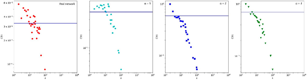
Figure 9. Simulation network clustering coefficient - degree correlation distribution (α = 1, 2, 3).

The analysis of the structural characteristics of the simulated network can be seen (Table 2), with the increase of α value, the average degree and network density remain unchanged, the average path length decreases. It indicates that the network tends to be closely connected. The average clustering coefficient increases, and the trade connectivity of countries increases. The number of degree off links (Pearson) decreases significantly, indicating that the characteristics of the heterogeneous network are amplified. Network modularity is used to detect the community structure of the network. The higher the modularity, the better the structure of the divided community. If the modularity is 0 or negative, it means the whole network is a single community or each node is a separate community. Among them, the modularity degree when α = 2 and 3 is 0, and the community structure does not match the real network. Meanwhile, the average path length and clustering coefficient at α = 1 are closer to the real network, therefore, α = 1 is selected for the next analysis.

Table 2

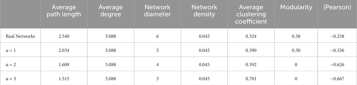
Table 2. Statistics of basic characteristics of simulated networks (α = 1, 2, 3).

Specifically, when the parameters α and ε are both set to 1 Among them, ε = 0.5, ε = 1 when all nodes of the network are connected, and ε = 2 when some nodes of the network are not connected (Figure 10). As the value of ε increases and the geographic restriction strengthens, the network hierarchy gradually weakens (Figure 11). When the geographic factor strengthens, the network becomes homogeneous and the phenomenon of degree negative correlation gradually disappears, such as when ε = 2, the nearest neighbor average degree value is almost a constant, indicating that the network has no degree correlation (Figure 12).

Figure 10

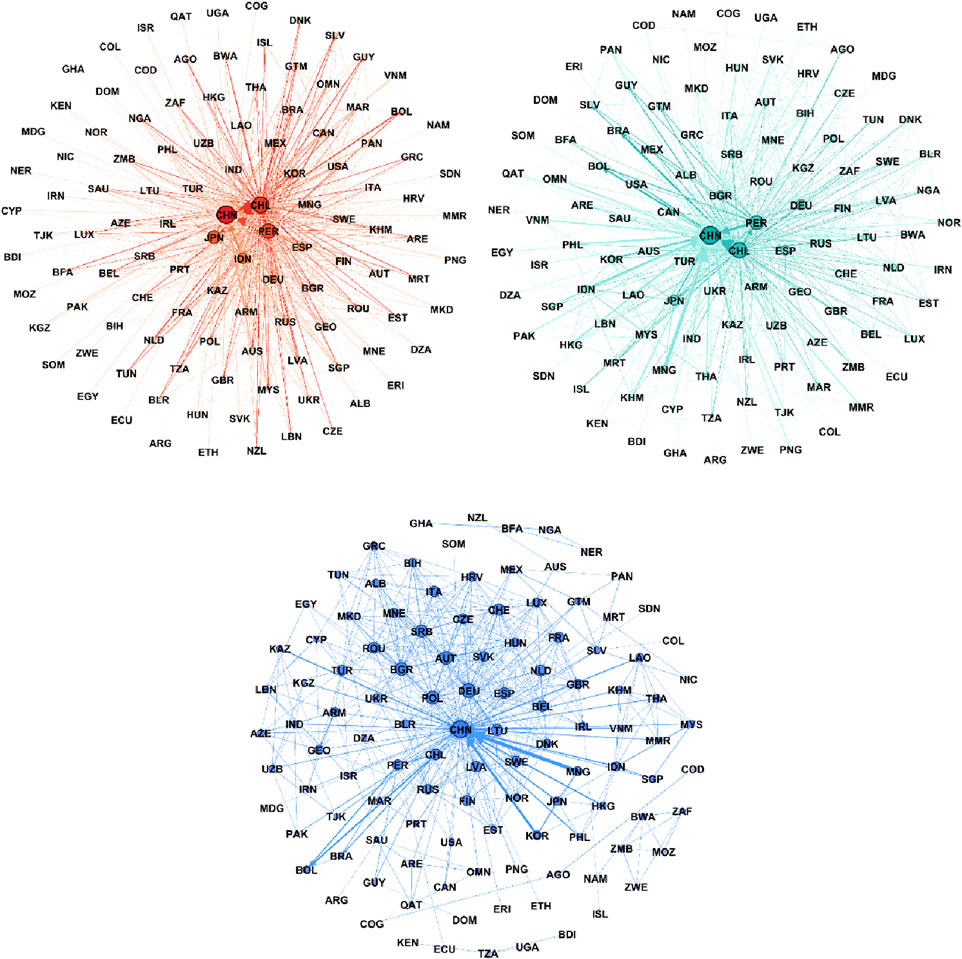
Figure 10. Global copper supply chain network model (ε = 0.5, 1, 2).

Figure 11

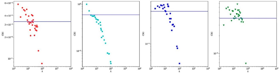
Figure 11. Simulation network clustering coefficient-degree correlation distribution (ε = 0.5, 1, 2).

Figure 12

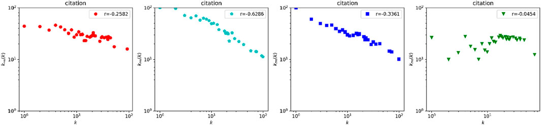
Figure 12. Simulation network degree - degree correlation distribution (ε = 0.5, 1, 2).

Combined with the above comparison, the basic structural characteristics of the statistical simulation network (Table 3) show that as the value of ε increases, the average path length increases, the network diameter increases, the network density remains the same, the average clustering coefficient becomes smaller, the modularity becomes smaller, and the hierarchical and community characteristics of the network gradually disappear.

Table 3

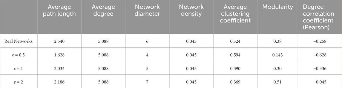
Table 3. Statistics of basic characteristics of simulated networks (ε = 0.5, 1, 2).

When ε is set to 1, the model network is closer to the real network, and the nodes with higher weighting degree include China, Chile, Peru Japan, and Indonesia. They are completely consistent with the real network. There are 17 of the top 20 countries in the weighted degree are consistent with the real network (Figure 13). It proves that the model can basically describe the driving pattern of establishing trade links between nodes. This model relates positively to the anticipated trade flow between nations and inversely to the intervening distance. It indicates that trade demand and the spatial distance are main driving forces for establishing trade ties among countries. Usually, trade ties are established with neighboring exporting countries that are relatively close in distance. With the increase in trade demand, the cost is limited, there will always be priority investment in the construction of the most urgent, the largest demand for trade flow. On this foundation, a scientific evaluation of the stability and potential risks associated with supply chain structures can be undertaken.

Figure 13

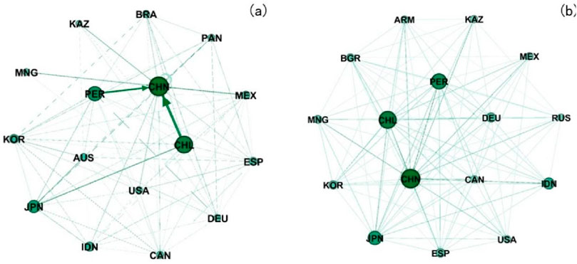
Figure 13. Global copper supply chain simulation network. [(A) original network, (B) simulation network].

The model reflects the ideal structure of the global copper ore trade network. But the trade relationships in the real network are simultaneously influenced by many factors, such as national geopolitical relations, market prices, import and export policies, regional trade agreements and others. There are some different relationships from the simulation results in this paper. The nodes in the real network that have not yet established trade links deserve further focused attention.

3.4 Forecast of potential trading countries

In recent years, China has been the world’s largest importer of copper ore. In this paper China is taken as an example to forecast the potential trading countries using the spatial weighted complex network model proposed above. Based on the data of 2021, the above model is used to simulate the evolution of the global copper supply chain structure and predict the changes of the global copper supply chain structure in 2022. The simulation results are compared with the real network to evaluate the accuracy of the model.

In 2021, China imported 23 million tons of copper ore from 59 countries. The major exporting countries are Chile, Peru, Kazakhstan, Mongolia, Mexico, Indonesia. These countries above account for nearly 80% of China’s copper imports. The spatial weighted complex network model was used with α = 1 and ε = 1. According to the simulation results, in 2022, there was little change in the major exporting countries, such as Chile, Peru, Kazakhstan, Mongolia, Mexico, Indonesia (Figure 14). And these countries above account for nearly 80% of China’s copper imports (Figure 15).

Figure 14

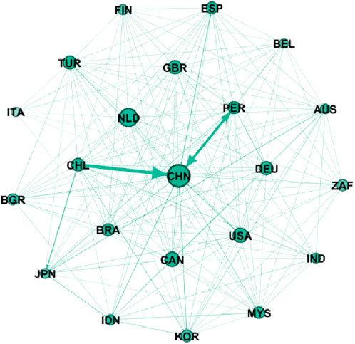
Figure 14. Global copper supply chain in 2022.

Figure 15

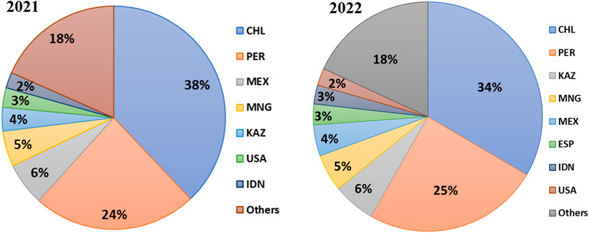
Figure 15. Source of China’s copper imports in 2021 and 2022.

From the perspective of network structure, China’s copper imports come from more diverse sources. The number of countries trading copper with China has grown to 83 in 2022. These include 80 countries in the list of countries simulated, the percentage is as high as 96%. This can also show that with the change of the global geographical situation, China is seeking new trading partners, expand the diversity of copper import sources, and more countries have joined the copper trade with China.

4 Conclusion

Based on the global copper ore trade import and export data from 1990 to 2022, this paper constructs a global copper ore trade network model using complex network theory. The historical evolution characteristics and structural change patterns of the global copper ore trade network are analyzed. The evolution process of the global copper ore trade network structure is simulated using a spatially weighted complex network model. Based on these findings, we propose an evolution pattern for the global copper ore trade network under the joint influence of national trade demand and transportation costs. The main conclusions drawn in this paper are as follows:

(1) The spatial heterogeneity in the distribution of mineral resources among exporting nations, coupled with the economic progress of importing countries, exerts a profound influence on the evolution of the global trade network structure. Major importing economies, notably Japan, China, Germany, and Spain, primarily procure copper resources from significant trade partners such as Chile and Canada. Concurrently, these importing nations are diversifying their import bases to encompass resource-rich countries situated in closer geographic proximity, thereby enhancing their supply chain resilience and strategic sourcing capabilities within the global trade framework.

(2) Since 1990, the total volume of global copper ore trade has exhibited a sustained growth trajectory, accompanied by a gradual expansion of the global copper ore trade network. The degree of network closeness exhibits fluctuations that are contingent upon the rate of this expansion. Notably, the small-world and heterogeneous attributes of the network have become increasingly apparent, underscoring an intensification of trade connectivity among nations.

(3) The evolutionary pattern of the global copper ore trade network can be accurately characterized using the spatial weighted complex network evolution model. This model relates positively to the anticipated trade flow between nations and inversely to the intervening distance. When both parameters α and ε are set to 1, the structure of the simulated copper ore trade network aligns more closely with the real network. On this foundation, a scientific evaluation of the stability and potential risks associated with supply chain structures can be undertaken.

Building upon the insights gained from our preceding analysis, we undertake a comprehensive examination of the structural attributes and evolutionary forces shaping the global copper supply chain. Subsequently, we offer a suite of strategic recommendations targeted at optimizing the international copper trade dynamics at a comprehensive level. Presently, the exportation of global copper ore is predominantly concentrated in key regions such as Chile, Peru, Indonesia, Mexico, and Australia. The potential trade relationships projected from this concentration merit particular scrutiny. It is advisable for importing countries such as China, Japan, Rep. of Korea, Spain, Germany to diversify copper sources and securing a stable supply chain. And suggestions for export countries such as Chile, Peru, Indonesia, Mexico, Australia to enhance production resilience and maintain trade advantages. For major trade intermediary countries such as the Netherlands, United Arab Emirates, Turkey, it is essential to stabilize the trade partnerships established with other nodes and actively expand their coverage and influence within the network. Furthermore, establishing copper trade relations with neighboring countries is recommended as a strategic approach to ensure the stability and resilience of the supply chain.

Data availability statement

The original contributions presented in the study are included in the article/supplementary material, further inquiries can be directed to the corresponding author.

Author contributions

QC: Conceptualization, Formal Analysis, Funding acquisition, Project administration, Writing–original draft, Writing–review and editing. KW: Conceptualization, Formal Analysis, Methodology, Writing–original draft, Writing–review and editing. YZ: Methodology, Software, Writing–review and editing. QG: Methodology, Software, Writing–original draft. JX: Data curation, Visualization, Writing–original draft. TL: Data curation, Visualization, Writing–original draft. GZ: Supervision, Writing–review and editing. QL: Project administration, Supervision, Writing–review and editing. ZL: Project administration, Supervision, Writing–review and editing. XR: Data curation, Writing–original draft. CS: Data curation, Writing–original draft. YD: Methodology, Software, Writing–original draft.

Funding

The author(s) declare that financial support was received for the research, authorship, and/or publication of this article. This work was supported by National Natural Science Foundation of China (NSFC) [grant numbers 42271281]; Deep Earth Probe and Mineral Resources Exploration - National Science and Technology Major Project [2024ZD1002006]; China Geological Survey, Ministry of Natural Resources [grant number DD20230040; DD20221694; DD20211405]; and Chinese Academy of Engineering strategic research and consulting project [grant numbers 52922023002].

Acknowledgments

The authors thank the reviewers for helpful comments on the draft manuscript.

Conflict of interest

The authors declare that the research was conducted in the absence of any commercial or financial relationships that could be construed as a potential conflict of interest.

Generative AI statement

The author(s) declare that no Generative AI was used in the creation of this manuscript.

Publisher’s note

All claims expressed in this article are solely those of the authors and do not necessarily represent those of their affiliated organizations, or those of the publisher, the editors and the reviewers. Any product that may be evaluated in this article, or claim that may be made by its manufacturer, is not guaranteed or endorsed by the publisher.

References

1. Kumar BH, Reddy NR, Kumar MCS. Cu-rich copper indium sulfide thin films deposited by co-evaporation for photovoltaic applications. J Mater Sci Mater Electronics (2023) 34:341. doi:10.1007/s10854-022-09441-w

CrossRef Full Text | Google Scholar

2. Abbas S, Saqib N, Shahzad U. Global export flow of Chilean copper: the role of environmental innovation and renewable energy transition. Geosci Front (2024) 15:101697. doi:10.1016/j.gsf.2023.101697

CrossRef Full Text | Google Scholar

3. Tang J, Yang H, Chen H, Li F, Wang C, Liu Q, et al. Potential and future direction for copper resource exploration in China. Green Smart Mining Eng (2024) 1:127–31. doi:10.1016/j.gsme.2024.06.001

CrossRef Full Text | Google Scholar

4. Rivera N, Guzmán J, Jara J, Lagos G. Evaluation of econometric models of secondary refined copper supply. Resour Pol (2021) 73:102170. doi:10.1016/j.resourpol.2021.102170

CrossRef Full Text | Google Scholar

5. Alexander D, Merkert R. Applications of gravity models to evaluate and forecast US international air freight markets post-GFC. Transport Policy (2021) 104:52–62. doi:10.1016/j.tranpol.2020.04.004

PubMed Abstract | CrossRef Full Text | Google Scholar

6. Guj P, Schodde R. Will future copper resources and supply be adequate to meet the net zero emission goal? Geosystems and Geoenvironment (2025) 4:100320. doi:10.1016/j.geogeo.2024.100320

CrossRef Full Text | Google Scholar

7. Kang X, Wang M, Wang T, Luo F, Lin J, Li X. Trade trends and competition intensity of international copper flow based on complex network: from the perspective of industry chain. Resour Pol (2022) 79:103060. doi:10.1016/j.resourpol.2022.103060

CrossRef Full Text | Google Scholar

8. Guan Q, An H. The exploration on the trade preferences of cooperation partners in four energy commodities’ international trade: crude oil, coal, natural gas and Photovoltaic. Appl Energ (2017) 203:154–63. doi:10.1016/j.apenergy.2017.06.026

CrossRef Full Text | Google Scholar

9. Chen Z, An H, An F, Guan Q, Hao X. Structural risk evaluation of global gas trade by a network-based dynamics simulation model. Energy (2018) 159:457–71. doi:10.1016/j.energy.2018.06.166

CrossRef Full Text | Google Scholar

10. Nassar N, Brainard J, Gulley A, Manley R, Matos G, Lederer G, et al. Evaluating the mineral commodity supply risk of the U. S. manufacturing sector. Sci Adv (2020) 6:8647. doi:10.1126/sciadv.aay8647

PubMed Abstract | CrossRef Full Text | Google Scholar

11. Althaf S, Babbitt C. Disruption risks to material supply chains in the electronics sector. Resour Conservation and Recycling (2020) 167:105248. doi:10.1016/j.resconrec.2020.105248

CrossRef Full Text | Google Scholar

12. Ryter J, Fu X, Bhuwalka K, Roth R, Olivetti EA. Emission impacts of China’s solid waste import ban and COVID-19 in the copper supply chain. Nat Commun (2021) 12:3753. doi:10.1038/s41467-021-23874-7

PubMed Abstract | CrossRef Full Text | Google Scholar

13. Brink S, Kleijn R, Sprecher B, Tukker A. Identifying supply risks by mapping the cobalt supply chain. Resour Conservation and Recycling (2020) 156:104743. doi:10.1016/j.resconrec.2020.104743

CrossRef Full Text | Google Scholar

14. Pizarro J, Sainsbury B, Hodgkinson J. Adaptation options assessment for the Australian uranium supply chain focused on the Olympic Dam and Ranger Mines. Environ Development (2020) 37:100610. doi:10.1016/j.envdev.2020.100610

CrossRef Full Text | Google Scholar

15. Mou M, Zhou Y, Zheng W, Xie Y. Integration and modeling of multi-energy network based on energy hub. Complexity (2022) 2022:2698226. doi:10.1155/2022/2698226

CrossRef Full Text | Google Scholar

16. Schnebele E, Jaiswal K, Luco N, Nassar N. Natural hazards and mineral commodity supply: quantifying risk of earthquake disruption to South American copper supply. Resour Pol (2019) 63:101430. doi:10.1016/j.resourpol.2019.101430

CrossRef Full Text | Google Scholar

17. Zhang H, Xi W, Ji Q, Zhang Q. Exploring the driving factors of global LNG trade flows using gravity modelling. J Clean Prod (2018) 172:508–15. doi:10.1016/j.jclepro.2017.10.244

CrossRef Full Text | Google Scholar

18. Shen J, Huang S. Copper cross-market volatility transition based on a coupled hidden Markov model and the complex network method. Resour Pol (2022) 75:102518. doi:10.1016/j.resourpol.2021.102518

CrossRef Full Text | Google Scholar

19. Ye H, Li Z, Li G, Liu Y. Topology analysis of natural gas pipeline networks based on complex network theory. Energies (2022) 15:3864. doi:10.3390/en15113864

CrossRef Full Text | Google Scholar

20. Hao M, Tang L, Wang P, Wang H, Wang Q, Dai T, et al. Mapping China's copper cycle from 1950-2015: role of international trade and secondary resources. Resour Conservation Recycling (2023) 188:106700. doi:10.1016/j.resconrec.2022.106700

CrossRef Full Text | Google Scholar

21. Yuan ZW, Ji HR, Zhang L, Liu L. Sustaining the United States’ copper resource supply. J Clean Prod (2023) 429:139636. doi:10.1016/j.jclepro.2023.139636

CrossRef Full Text | Google Scholar

22. Zhang W, Ye Y, Li Z, Xian J, Wang T, Liu D, et al. The coupled awareness-epidemic dynamics with individualized self-initiated awareness in multiplex networks. Front Phys (2024) 12:1437341. doi:10.3389/fphy.2024.1437341

CrossRef Full Text | Google Scholar

23. Suárez V, Montoya-Torres J, Sepúlveda-Rojas J. A gravitational model extended by institutional and cultural factors for Colombian foreign trade. Management Sci Lett (2021) 11:2313–22. doi:10.5267/J.MSL.2021.6.003

CrossRef Full Text | Google Scholar

24. Duenas M, Fagiolo G. Global trade imbalances: a network approach. Advcomplex Syst (2014) 17:1450014. doi:10.1142/S0219525914500143

CrossRef Full Text | Google Scholar

25. Zhang YT, Zhou WX. Structural evolution of international crop trade networks. Front Phys (2022) 10:926764. doi:10.3389/fphy.2022.926764

CrossRef Full Text | Google Scholar

26. Liu M, Guo Q, Liu J. Effect of network structure on the accuracy of resilience dimension reduction. Front Phys (2024) 12:1420556. doi:10.3389/fphy.2024.1420556

CrossRef Full Text | Google Scholar

27. Li B, Li H, Ren S, Liu H, Wang G. Commodity supply risk assessment of China’s copper industrial chain: the perspective of trade network. Resour Pol (2023) 81:103297. doi:10.1016/j.resourpol.2023.103297

CrossRef Full Text | Google Scholar

28. Barabási AL. Network science. Cambridge University Press (2016).

Google Scholar

29. Zhang L, Jian X, Ma Y. Analysis of differences in fossil fuel consumption in the world based on the fractal time series and complex network. Front Phys (2024) 12:1457287. doi:10.3389/fphy.2024.1457287

CrossRef Full Text | Google Scholar

30. Ma Y, Wang MX, Li X. Analysis of the characteristics and stability of the global complex nickel ore trade network. Resour Pol (2022) 79:103089. doi:10.1016/j.resourpol.2022.103089

CrossRef Full Text | Google Scholar

31. Xi X, Zhou J, Gao X, Liu D, Zheng H, Sun Q. Impact of changes in crude oil trade network patterns on national economy. Energy Econ (2019) 84:104490. doi:10.1016/j.eneco.2019.104490

CrossRef Full Text | Google Scholar

32. Aydın U, ülengin B. Analyzing air cargo flows of Turkish domestic routes: a comparative analysis of gravity models. J Air Transport Management (2022) 102:102217. doi:10.1016/j.jairtraman.2022.102217

CrossRef Full Text | Google Scholar

33. Chenaf-Nicet D, Rougier E. The effect of macroeconomic instability on FDI flows: a gravity estimation of the impact of regional integration in the case of Euro-Mediterranean agreements. Int Econ (2016) 145:66–91. doi:10.1016/j.inteco.2015.10.002

CrossRef Full Text | Google Scholar

34. Kwon O, Jung W. Intercity express bus flow in Korea and its network analysis. Physica A: Stat Mech its Appl (2012) 391:4261–5. doi:10.1016/j.physa.2012.03.031

CrossRef Full Text | Google Scholar

35. Lundmark R. Analysis and projection of global iron ore trade: a panel data gravity model approach. Miner Econ (2018) 31:191–202. doi:10.1007/s13563-017-0125-8

CrossRef Full Text | Google Scholar

36. Akerman A, Leuven E, Mogstad M. Information frictions, internet, and the relationship between distance and trade. Am Econ J Appl Econ (2022) 14:133–63. doi:10.1257/app.20190589

CrossRef Full Text | Google Scholar

37. Hsieh TH, Zhu YB, Huang KL. Using the gravitational mixed models to analyze the impact of China’s foreign direct investment along with the Belt and Road countries on trade flows. Front Psychol (2022) 13:960722. doi:10.3389/fpsyg.2022.960722

PubMed Abstract | CrossRef Full Text | Google Scholar

38. Zhao N, Liu Q, Wang H, Yang SL, Li PZ, Wang J. Estimating the relative importance of nodes in complex networks based on network embedding and gravity model. J King Saud Univ - Computer Inf Sci (2023) 35:101758. doi:10.1016/j.jksuci.2023.101758

CrossRef Full Text | Google Scholar

39. Dabbaghfeizi S, Naderan A, Tavakoli-Kashani A. Aggregate crash prediction model based on gravity model: introducing crash risk distribution concept. Transportation Eng (2025) 19:100297. doi:10.1016/j.treng.2024.100297

CrossRef Full Text | Google Scholar