Single-epoch power positioning method for multi-beam LEO communication satellites

Low Earth Orbit (LEO) communication satellites offer reduced signal loss, fast movement, multi-beam, typically providing single coverage. This paper introduces a novel multi-beam power positioning method for low-orbit single-satellite, addressing the slow convergence and low accuracy of Doppler positioning. It establishes a power observation equation system, initializes with the nearest neighbor algorithm, and refines with the least squares method. Monte Carlo simulations indicate that with good initial values, the method converges in under 10 iterations, achieving 88.06% availability at 20° elevation with errors of 5,331 m (vertical) and 8,798 m (horizontal), and a timing error of 205 μs. At 70° elevation, all users converge with errors of 1,614 m and 1,088 m, and a timing error of 31.3 μs, demonstrating high power positioning availability. The statistical results show that power positioning users can obtain the positioning accuracy of kilometers and the timing accuracy of microseconds, which meets initial timing needs under strong confrontation, enhancing the medium and high orbit satellite navigation.

1 Introduction

Low Earth Orbit (LEO) communication satellites, as an emerging navigation enhancement method, possess many unique advantages. Their orbital altitude is relatively low, and the signal power is high, with the ground power being about 30 dB higher than that of Global Navigation Satellite System (GNSS), resulting in high signal quality and strong anti-interference capabilities, enabling services to be provided indoors and in obstructed areas [1, 2]. The greatest advantage of LEO satellites is their fast movement speed, which can greatly reduce the correlation between adjacent observation epochs, achieving rapid convergence in positioning [3], and the large Doppler shift, which offers good Doppler observation [4].

Based on the characteristics of LEO satellites, with a sufficient number of satellites, LEO navigation constellations can perform independent positioning and timing, or combined positioning and timing with GNSS, using traditional positioning algorithms such as pseudorange positioning and carrier phase positioning to achieve navigation enhancement [5–7]. The analysis of the combined positioning effects of LEO satellites with different orbital heights and GNSS constellations [8] shows that LEO satellites have low orbits and fast geometric motion speeds, with the geometric dilution of precision (GDOP) value changing rapidly, effectively shortening the convergence time for GPS/BDS positioning. The enhancement effect of different numbers of LEO satellites on GNSS is significantly different, with more satellites leading to more noticeable enhancement effects.

However, for LEO satellite constellations, if the GNSS pseudorange-based time difference positioning method is still used, the system’s requirement for time synchronization is very high, which will greatly increase the system construction cost [9]. When the number of visible satellites is insufficient, and users do not meet the conditions for multiple coverage, both pseudorange positioning and carrier phase positioning are not available. In this case, single-satellite Doppler positioning requires a relatively long observation time for the satellite, using integrated Doppler for positioning solution, which is not real-time [10], has a long convergence time, and low precision, and has certain application limitations. In LEO-based Doppler positioning, the pioneering TRANSIT navigation system was the first satellite-based Doppler positioning system [11]. Launched in 1964 for military applications, it was later released for public use in 1968 to provide positioning and navigation services [12]. The system operated with over 10 satellites in polar orbits at an altitude of approximately 1,100 km. Typically, a receiver could only track one satellite at a time. Using about 2 min of Doppler shift observations, the point positioning accuracy was about 100–200 m. With the advent of the Global Positioning System (GPS) and its superior performance, TRANSIT was decommissioned in 1996.

To meet the rapid positioning needs of LEO users, the power measurements of multi-beam signals can be utilized to calculate the user’s approximate location. Due to the beam scanning broadcast method used by LEO communication satellites [13], there are variations in received power for receivers at different locations on the Earth’s surface at various times during the satellite’s motion. The magnitude of these variations is related to the beamwidth and the antenna pattern. Current research on power matching positioning is focused on indoor positioning, where multiple WiFi access points can be detected indoors and their signals are easily measured, making WiFi received signal strength indication based fingerprint positioning one of the most popular positioning technologies today [14]. This method typically consists of two stages: offline and online [15, 16]. In the offline stage, reference points in the positioning area are surveyed to collect received signal strength as a fingerprint database [17, 18]; in the online stage, real-time positioning data are matched with the fingerprint database to obtain the estimated location [19].

For the first time in the context of LEO satellite scenarios, this paper proposes the use of multi-beam signal power measurements for positioning and timing. Based on traditional satellite navigation system algorithms, the nearest neighbor algorithm [20, 21] is used to solve for initial values, and the least squares method [22] is used for iterative solution, including the linearization of nonlinear equation systems, solution of linear equation systems, updating the roots of nonlinear equation systems, and judging the convergence of iterations. It is possible to use power measurements for single-point rapid positioning of users under a single LEO satellite scenario, with the expectation that some users will achieve better positioning and timing performance.

2 Materials and methods

2.1 Multi-beam signal power observation model

According to the classic Friis transmission equation, the power measurement of the multi-beam satellite signal received by the satellite azimuth angle $\beta$, the satellite elevation angle $\gamma$ and the distance between the user and the satellite $d$, which can be expressed as:

$P_k\left(\gamma ,\beta ,d\right)=E_k\left(\gamma ,\beta \right)-L\left(d\right)+G\left(\gamma \right)(1)$

Among them, the multi-beam number $k=1,\cdots ,M$ representing the signal transmitted by the satellite. $E_k\left(\gamma ,\beta \right)$ represents the EIRP value of the satellite transmitted signal, $L\left(d\right)$ represents the spatial transmission loss of the satellite signal, and $G\left(\alpha \right)$ represents the gain value of the user’s receiving antenna, which is solely related to the user’s elevation angle $\alpha$ and can be calculated using the satellite elevation angle $\gamma$.

The EIRP value of the satellite transmitted beam signal and the gain value of the user’s received antenna $E_k\left(\gamma ,\beta \right)$, $G\left(\gamma \right)$ can usually be obtained by antenna simulation or actual measurement, and it is assumed that the accurate modeling of both has been completed, and the modeling error is ignored.

When the satellite position is known, the user’s position can be determined by the satellite elevation angle $\gamma$, the satellite azimuth angle $\beta$ and the distance $d$ between the user and the satellite, and when the three-dimensional position of the satellite in the ECEF coordinate system is known, the three-dimensional position of the user in the ECEF coordinate system can be obtained by using the geometric relation. Figure 1 below shows the geometric relationship between the user and the satellite, where $R$ is the radius of the earth, $H$ is the orbital height of the satellite, $h$ is the geodetic height of the user, and $d$ is the distance between the user and the satellite. Firstly, the relationship between the elevation angle of the user and the expansion angle of the satellite beam is derived.

Figure 1

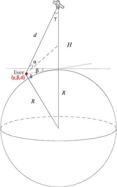
Figure 1. Geometry of the user’s received satellite signal.

The geometric relationship shown in the figure above, according to the sinusoidal theorem, can be obtained:

$\left(R+H\right)\sin \gamma =\left(R+h\right)\sin \left(\alpha +\frac{\pi }{2}\right)(2)$

Therefore, it is possible to derive the satellite beam tension angle $\gamma$ as Equation 3:

$\gamma ={\sin }^{-1}\left(\frac{R+h}{R+H}\cos \alpha \right)(3)$

When the elevation angle of the user is valued between 0° and 90°, it is not difficult to conclude that the elevation angle of the user corresponds to the value of the satellite elevation angle from the function relationship.

The space transmission loss of satellite signals $L\left(\alpha ,h\right)$ is deduced below, and the distance from the satellite to the user is calculated first. According to the geometric relationship shown in Figure 1, and according to the cosine theorem, we can get:

${\left(R+H\right)}^2={\left(R+h\right)}^2+d^2-2d\left(R+h\right)\cos \left(\alpha +\frac{\pi }{2}\right)(4)$

Further, the distance from the user to the satellite $d$ can be calculated as:

$d=\sqrt{{\left(R+H\right)}^2-{\left(R+h\right)}^2{\cos }^2\alpha }-\left(R+h\right)\sin \alpha (5)$

According to Friis transmission equation, the power in the fixed solid angle remains the same. Therefore, the spatial transmission loss of signal power at a point on the spherical surface with a radial of the transmitting antenna is Equation 6:

$L\left(\alpha ,h\right)=L\left(d\right)=20\lg \left(4\pi d\right)-20\lg \left(\lambda \right)(6)$

where $\lambda$ refers to the wavelength.

Thus, Equation 1 can be written in a more detailed form as Equation 7:

$P_k\left(\alpha ,\gamma ,\beta ,h\right)=E_k\left(\gamma ,\beta \right)-L\left(\alpha ,h\right)+G\left(\alpha \right)(7)$

2.2 Power perception measurement error model

After receiving the signal from the satellite, the user usually measures the power of the received signal by matching the reception. Assuming that the user has completed the time and frequency synchronization of the satellite signal, and stripped away the possible pseudo-random codes and Doppler frequencies that may be modulated on the signal, while ignoring the influence of the transmitted message symbol, the user’s received signal can be expressed as Equation 8:

$s\left(t\right)=A+n\left(t\right)(8)$

where the amplitude of the received signal is denoted by $A=\sqrt{2P_k\left(\alpha ,\gamma ,\beta ,h\right)}$, the thermal noise error of the power is denoted by $n\left(t\right)$ which generally obeys a normal distribution [23].

Considering that the thermal motion of charged particles in a circuit forms thermal noise, the noise power $N$ is usually expressed as the noise temperature $T$ corresponding to the thermal noise power of the same magnitude, and the relationship between them is as Equation 9:

$N=kT{B}_n(9)$

The unit of $N$ is Watts(W), the unit of $T$ is Kelvin (K) and the unit of noise bandwidth $B_n$ is Hertz (Hz). The Boltzmann constant $k$ is equal to $1.38\times {10}^{-23}$ J/K, which $T$ is taken as 290 K at room temperature.

When the duration of the signal power measurement is $T_P$, it is advisable to assume that the user takes the coherent integration method to estimate the signal amplitude, then there are:

$\widehat{A}=\frac{1}{T_P}{\int }_0^{T_P}s\left(t\right)dt=A+n^{\prime }\left(t\right)(10)$

where $\widehat{A}$ is the measured value of the amplitude of the received signal. $n^{\prime }\left(t\right)$ is the coherent integrated noise, and its equivalent noise bandwidth $B_n$ is taken $1/T_P$. Before and after coherent integration, the signal power, amplitude, and noise power spectral density do not change, but because the noise bandwidth before the correlator is $B_{pd}$, and the filtering bandwidth of the coherent integrator can be regarded as $B_n$ , the narrowing of the noise bandwidth must cause a decrease in the noise power, so the noise power after coherent integration is reduced to $N/B_{pd}{T}_P$.

2.3 A system of equations for power observations

When the user receives multiple beamed satellite signals and measures the signal power, the equation is as follows:

$\left\{\begin{array}{c}{E}_1\left(\gamma ,\beta \right)+L\left(d\right)+G\left(\alpha \right)+N_1^T={\widehat{P}}_1\\ E_2\left(\gamma ,\beta \right)+L\left(d\right)+G\left(\alpha \right)+N_2^T={\widehat{P}}_2\\ ⋮\\ E_M\left(\gamma ,\beta \right)+L\left(d\right)+G\left(\alpha \right)+N_M^T={\widehat{P}}_M\end{array}\right.(11)$

Among them, ${\widehat{P}}_1,{\widehat{P}}_2,\cdots ,{\widehat{P}}_M$ are the power measurement of different beams, and $N_1^T,N_2^T,\cdots ,N_M^T$ are the power observation noise of different beams.

The power observation equation for the other beams is different from the observation equation for beam 1, the difference between other beams and beam 1 is calculated by:

$\left\{\begin{array}{c}\Delta E_2\left(\gamma ,\beta \right)+N_2^T-N_1^T=\Delta {\widehat{P}}_2\\ \Delta E_3\left(\gamma ,\beta \right)+N_3^T-N_1^T=\Delta {\widehat{P}}_3\\ ⋮\\ \Delta E_M\left(\gamma ,\beta \right)+N_M^T-N_1^T=\Delta {\widehat{P}}_M\end{array}\right.(12)$

where, take $∆E_k\left(\alpha ,\beta \right)=E_k\left(\alpha ,\beta \right)-E_1\left(\alpha ,\beta \right)$, $∆{\widehat{P}}_k={\widehat{P}}_k-{\widehat{P}}_1$.

Assuming that the initial values of $\gamma$ and $\beta$ are ${\gamma }_0$ and ${\beta }_0$ ,where the system of equations is linearized and expanded, then there is:

$\left\{\begin{array}{c}\Delta E_2\left({\gamma }_0,{\beta }_0\right)+\left(\gamma -{\gamma }_0\right){\left.\frac{\mathrm{\partial }\Delta E_2}{\mathrm{\partial }\gamma }\right|}_{\left({\gamma }_0,{\beta }_0\right)}+\left(\beta -{\beta }_0\right){\left.\frac{\mathrm{\partial }\Delta E_2}{\mathrm{\partial }\beta }\right|}_{\left({\gamma }_0,{\beta }_0\right)}+\Delta N_2^T=\Delta {\widehat{P}}_2\\ \Delta E_3\left({\gamma }_0,{\beta }_0\right)+\left(\gamma -{\gamma }_0\right){\left.\frac{\mathrm{\partial }\Delta E_3}{\mathrm{\partial }\gamma }\right|}_{\left({\gamma }_0,{\beta }_0\right)}+\left(\beta -{\beta }_0\right){\left.\frac{\mathrm{\partial }\Delta E_3}{\mathrm{\partial }\beta }\right|}_{\left({\gamma }_0,{\beta }_0\right)}+\Delta N_3^T=\Delta {\widehat{P}}_3\\ ⋮\\ \Delta E_M\left({\gamma }_0,{\beta }_0\right)+\left(\gamma -{\gamma }_0\right){\left.\frac{\mathrm{\partial }\Delta E_M}{\mathrm{\partial }\gamma }\right|}_{\left({\gamma }_0,{\beta }_0\right)}+\left(\beta -{\beta }_0\right){\left.\frac{\mathrm{\partial }\Delta E_M}{\mathrm{\partial }\beta }\right|}_{\left({\gamma }_0,{\beta }_0\right)}+\Delta N_M^T=\Delta {\widehat{P}}_M\end{array}\right.(13)$

where $∆N_k^T=N_k^T-N_1^T$, and cause:

$\mathit{X}={\left[\begin{array}{cccc}{\left.\frac{\mathrm{\partial }\Delta E_2}{\mathrm{\partial }\gamma }\right|}_{\left({\gamma }_0,{\beta }_0\right)}& {\left.\frac{\mathrm{\partial }\Delta E_3}{\mathrm{\partial }\gamma }\right|}_{\left({\gamma }_0,{\beta }_0\right)}& \cdots & {\left.\frac{\mathrm{\partial }\Delta E_M}{\mathrm{\partial }\gamma }\right|}_{\left({\gamma }_0,{\beta }_0\right)}\\ {\left.\frac{\mathrm{\partial }\Delta E_2}{\mathrm{\partial }\beta }\right|}_{\left({\gamma }_0,{\beta }_0\right)}& {\left.\frac{\mathrm{\partial }\Delta E_3}{\mathrm{\partial }\beta }\right|}_{\left({\gamma }_0,{\beta }_0\right)}& \cdots & {\left.\frac{\mathrm{\partial }\Delta E_M}{\mathrm{\partial }\beta }\right|}_{\left({\gamma }_0,{\beta }_0\right)}\end{array}\right]}^T(14)$

$\mathit{y}={\left[\Delta {\widehat{P}}_2-\Delta E_2\left({\gamma }_0,{\beta }_0\right),\Delta {\widehat{P}}_3-\Delta E_3\left({\gamma }_0,{\beta }_0\right),\cdots ,\Delta {\widehat{P}}_M-\Delta E_M\left({\gamma }_0,{\beta }_0\right)\right]}^T(15)$

$\mathit{n}={\left[N_1^T-N_2^T,N_1^T-N_3^T,\cdots ,N_1^T-N_M^T\right]}^T(16)$

Then the above equation can be rewritten as:

$\mathit{X}\cdot {\left[\gamma -{\gamma }_0,\beta -{\beta }_0\right]}^T=\mathit{y}+\mathit{n}(17)$

Further, it can be solved that:

${\left[\gamma ,\beta \right]}^T={\left[{\gamma }_0,{\beta }_0\right]}^T+{\mathit{X}}^{-1}\cdot \left(\mathit{y}+\mathit{n}\right)(18)$

Equations 11–18 are the derivation process of the least squares algorithm for power positioning. According to the properties of the least squares solution for linear systems of equations, the number of equations should be greater than or equal to the number of unknowns. Considering the unknowns are the satellite elevation angle $\gamma$ and the satellite azimuth angle $\beta$, the number of equations should be at least 2. Furthermore, since the linear system of equations is derived from the differentiation of different beams, the minimum number of satellite beams required by the algorithm is 3.

2.4 Power positioning algorithm solution process

Since multi-beam power positioning is applied to low-orbit satellite scenarios, the quality of the received signal is poor when the user’s elevation angle is too low, thus eliminating the data with low user elevation angles. In addition, according to the general specification for BeiDou/Global Navigation Satellite Systems (GNSS) geodetic receivers [24], typical values for navigation receiver acquisition and tracking sensitivities are generally below −130 dB m, thus the simulation parameters are set as Table 1:

Table 1

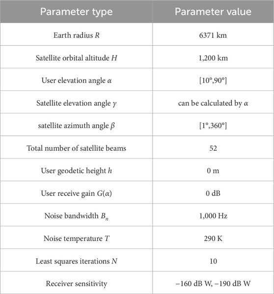
Table 1. Simulation parameters.

The input required for the power positioning least squares algorithm is the initial value of the satellite elevation angle ${\gamma }_0$, the initial value of the azimuth angle ${\beta }_0$, the ERIP value of k beams of prior information $E_k\left(\gamma ,\beta \right)$ , and the user gain $G\left(\alpha \right)$.Figure 2 gives the flowchart of the algorithm.

Figure 2

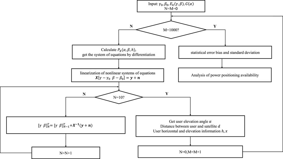
Figure 2. Flowchart of the power positioning least squares algorithm.

The least-squares algorithm itself outputs the satellite tension angle and azimuth angle, however, we need to obtain the user’s vertical and horizontal information. It is worth noticing that in the process of calculating the elevation angle of the user, $h=0$ is first assumed, which is due to the negligible altitude of the user’s geodetic altitude in relation to the radius of the Earth and the orbital height of the satellite. The h after the least squares solution is obtained by a series of calculations such as link loss, and the two values are not contradictory, and the analysis of the error in the following is based on the h of the least squares solution.

Substituting Equation 2, we can get the elevation angle from the user to the satellite as Equation 19:

$\alpha ={\cos }^{-1}\left\{\frac{R+H}{R+h}\sin \gamma \right\}(19)$

According to Equation 4, the user’s geodetic height can be calculated as Equation 20:

$h=-R-d\sin \alpha +\sqrt{{\left(R+H\right)}^2-d^2{\cos }^2\alpha }(20)$

where $d$ can be calculated by Equation 5, and the user vertical information is Equation 21:

$x=d\frac{\sin \gamma }{\sin \left(\alpha +\gamma \right)}(21)$

In order to facilitate the subsequent analysis of the power positioning and timing performance, the evaluation index of the positioning and timing result error is defined here, assuming that the true value of the satellite elevation angle is ${\gamma }_r$ and the solution value is $\gamma$ ,then the elevation angle error is $∆\gamma =\gamma -{\gamma }_r$.

If there are $n$ users in different locations, the statistical positioning performance of these users can be given by the error deviation and the standard deviation, which is defined as Equations 22, 23:

$E\left(\left|\Delta \gamma \right|\right)=\frac{1}{n}{\displaystyle \sum _n}\left|\gamma -{\gamma }_r\right|(22)$

$std\left(\Delta \gamma \right)=\sqrt{D\left(\Delta \gamma \right)}=\sqrt{\frac{1}{n-1}{\displaystyle \sum _n}{\left(\Delta \gamma -E\left(\Delta \gamma \right)\right)}^2}(23)$

Satellite azimuth error, user horizontal error, user vertical error and their deviation are defined as above.

Assuming the true distance between the user and the satellite is $d_r$, and the distance calculated by the power positioning algorithm between the user and the satellite is d, then the timing error is defined as Equation 24:

$\Delta t=\left|\frac{d_r-d}{c}\right|(24)$

where $c$ is the speed of light, which is approximately taken as $3\times {10}^{8}m·s^{-1}$.

3 Results

3.1 The requirements and acquisition of initial values in the least squares method

In the process of power positioning solution, the initial conditions have a great influence on the results, and the better initial conditions can make the iteration converge quickly, and the poor initial conditions will greatly reduce the iteration speed, and even the convergence results cannot be obtained in the end. Due to the characteristics of planar phased array antennas, ground users may have the same receiving power in different areas, and if the gap between the initial position and the user’s position is too large, the solution is easy to fall into the local optimal solution, resulting in a large positioning error.

3.1.1 Requirements for initial values in the least squares method

When the initial values are set close to the true values, the iteration tends to converge; when the initial values are set far from the true values, the least squares iteration diverges. Consequently, the power positioning least squares scheme has certain requirements for initial values.

To determine these requirements, it is assumed that the true elevation and azimuth angles of the satellite are $\left[\begin{array}{c}{\mathrm{\gamma }}_r\\ {\mathrm{\beta }}_r\end{array}\right]$, the initial value $\left[\begin{array}{c}{\mathrm{\gamma }}_r\pm a\\ {\mathrm{\beta }}_r\pm b\end{array}\right]$ is set to a certain value below the true value, and the positioning results $\left[\begin{array}{c}\mathrm{\gamma }\\ \mathrm{\beta }\end{array}\right]$ of multiple Monte Carlo simulations are required to converge to within the range of the true value of 1$°$, that is $\left[\begin{array}{c}{\mathrm{\gamma }}_r\pm 0.5°\\ {\mathrm{\beta }}_r\pm 0.5°\end{array}\right]$, the initial value requirements of the least squares method at this time are required a and b, where a is the initial value requirement of the satellite elevation angle, and b is the initial value requirement of the satellite azimuth angle.

In the simulation, users with poor observation quality due to low elevation angles are excluded. By iterating over user elevation angles $\alpha$ in the range [10°, 90°] (which corresponds to satellite elevation angles $\gamma$ in the range [0°, 55.8°]), and satellite azimuth angles $\beta$ in the range [1°, 360°], we can statistically determine the initial value requirements a and b for the power matching least squares method.

The statistical results of the initial value of least squares solution requirements are shown in Figure 3:

Figure 3

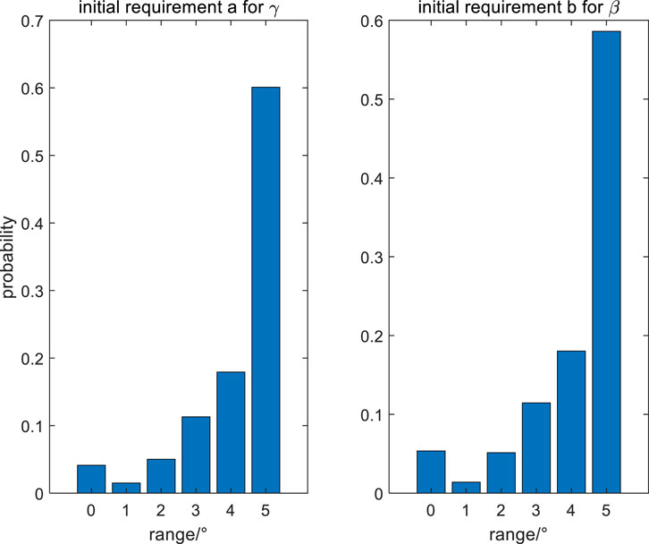
Figure 3. The proportion of users with different initial values required by the least squares algorithm.

It is not difficult to see that when the initial values of elevation angle and azimuth angle are below the true value of 2°, it can be considered that the vast majority of users (94.5% and 93.2%) can use power matching positioning to perform least squares solution and obtain a convergence solution. The solution to meet the initial value requirements can be obtained by using user prior information or other algorithms.

3.1.2 Acquisition of initial values by the nearest neighbor algorithm

This section introduces the method of obtaining the initial value that satisfies the convergence condition of least squares solution, and briefly explains the nearest neighbor algorithm (K value takes 1 in KNN) as an example, and then considers different fingerprint database frameworks and parameters.

According to the system of power measurement Equation 10, based on the EIRP information of each beam $\left(E_1,E_2,\cdots ,E_M\right)$ known on the satellite side, the theoretical received power values of users at different locations $\left(P_1,P_2,\cdots ,P_M\right)$ can be solved through the link budget, and in fact, for a single user, the received power of up to M beams $\left({\widehat{P}}_1,{\widehat{P}}_2,\cdots ,{\widehat{P}}_M\right)$ can be obtained. When the user’s fingerprint location information is the real user location, there will only be one noise deviation between the theoretical received power value of M and the actual received power value of a single user, which is very small and negligible in most cases, which is called positioning matching. However, when the user location fingerprint is different from the real user location, there will always be a large difference between the theoretical received power value and the actual received power value of some beams of a single user, which is called mismatch.

Considering the processing time of the nearest neighbor algorithm and the actual user situation, the power fingerprint database in this paper traverses the elevation angles of different users and takes a certain azimuth interval to establish it. In the matching process, the azimuth interval can be initialized by a priori known information, and then the azimuth search interval can be gradually narrowed to achieve more accurate and robust matching results.

In the simulation, we traverse the user’s elevation angle $\alpha ϵ\left[10°,90°\right]$ (converted to a satellite elevation angle of $\gamma ϵ\left[0,55.8°\right]$), the satellite azimuth angle $\beta ϵ\left[1°,360°\right]$, and the user’s ground height are all set to 0 m. Assuming that the user’s elevation angle is unknown and the azimuth uncertainty is 5$°$, there are 72 different fingerprint databases, each of which contains all the user’s elevation angle information and a certain azimuth information. In order to reduce the influence of noise on the nearest neighbor algorithm, the width of the fingerprint library is taken as 10 beams, which are the 10 largest beam points among the M received power obtained by each user.

The simulation results of the nearest neighbor algorithm power matching localization are as Figure 4.

Figure 4

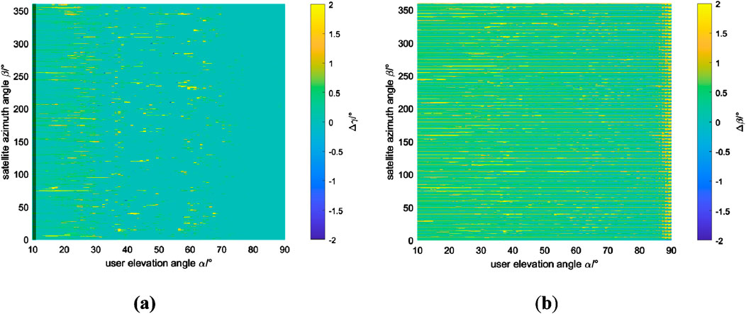
Figure 4. The Nearest Neighbor algorithm: (A) Satellite elevation angle errors (B) Satellite azimuth angle errors.

The colorbar depth of the above two graphs represents the azimuth and vertical error of the satellite, and the darker the color, the smaller the error. It can be seen that the error of satellite elevation angle is small, generally below 0.5$°$, while the azimuth error of satellite is large, generally above 0.5$°$, and the error under the condition of high user elevation angle is significantly increased, which is mainly due to the fact that the beam receiving power of users with high elevation angle is generally large, and it is difficult to distinguish the difference of beam between different users, resulting in some misjudgments in the algorithm. In general, the power matching positioning of the nearest neighbor algorithm can meet the requirements of the least-squares algorithm for the initial value of convergence.

3.2 Analysis of the single user positioning error

Assumed the satellite angle errors are $\left[\begin{array}{c}∆\gamma \\ ∆\beta \end{array}\right]$, the power calculation error is $∆p$,if error terms are taken into account as Equation 25:

$X\left[\begin{array}{l}\gamma +\Delta \gamma \\ \beta +\Delta \beta \end{array}\right]=y+n+\Delta p(25)$

From the previous Newtonian iterative process, it can be deduced that the relationship between the elevation angle and azimuth angle of the two satellites directly related to the user’s position and the power calculation error is as Equation 26:

$\left[\begin{array}{l}\Delta \gamma \\ \Delta \beta \end{array}\right]={\left(X^{T}X\right)}^{-1}{X}^T\Delta p(26)$

Assuming that the parameters remain unchanged during the receiver receiving the satellite signal, and each observation value is independent of each other, the observation error $∆p$ obeys the standard normal distribution, the mean value is 0, and the variance is ${\mathrm{\sigma }}^2$. So the covariance of $\left[\begin{array}{c}∆\gamma \\ ∆\beta \end{array}\right]$ can be expressed as Equation 27:

$Cov\left(\left[\begin{array}{l}\Delta \gamma \\ \Delta \beta \end{array}\right]\right)={\left(X^{T}X\right)}^{-1}{\sigma }^2(27)$

Taking the user’s elevation angle of 60$°$ (converted to a satellite elevation angle of 24.882$°$), the satellite azimuth angle of 30$°$, and the geodetic height of 0 m as an example, the receiver sensitivity is set to −160 dB W, and the results of multiple Monte Carlo simulations are as follows.

As can be seen from the Figure 5, the satellite tension angle and azimuth results of multiple Monte Carlo simulations are around the true value, and their statistical mean values can converge to within the range of 0.5$°$ of the true value. The vertical and horizontal error of a single Monte Carlo simulation is less than 40 km, and its statistical average value can converge to within the range of 50 km of the true value, and the power positioning algorithm tends to converge, so the user can use the power positioning timing method to perform multiple positioning solutions to achieve better positioning performance. The results of 1,000 Monte Carlo simulations are statistically analyzed, and the probability distribution functions of each parameter are fitted as follows in Figure 6.

Figure 5

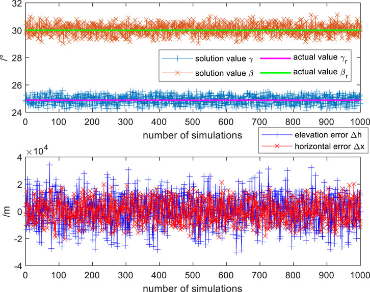
Figure 5. Monte Carlo results of $\gamma ,\beta ,∆h,∆x$.

Figure 6

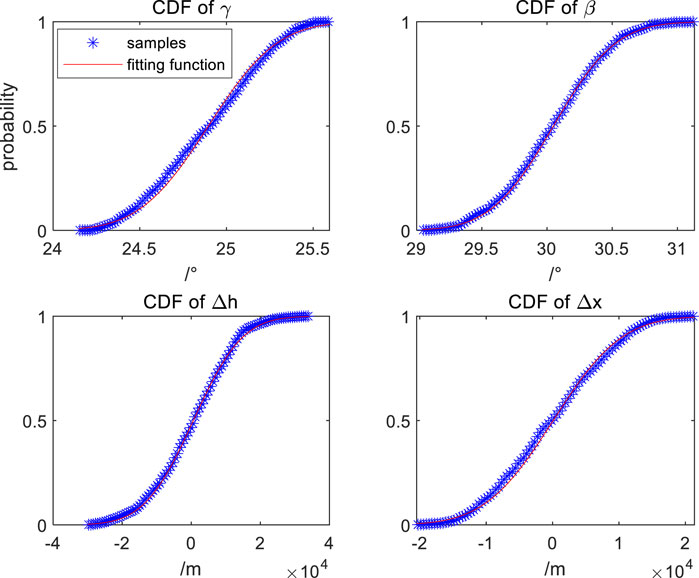
Figure 6. Normal distribution fits of Monte Carlo results.

The normal fitting of satellite azimuth angle $\beta$, user vertical difference $\Delta h$, and horizontal difference $\Delta x$ is good. The solved satellite azimuth angle $\beta$ is approximately normally distributed as $N\left(30.05,0.1426\right)$, and the elevation angle $\gamma$ is approximately normally distributed as $N\left(24.90,0.0976\right)$, with deviations of 0.03° and 0.038°, respectively. The user vertical difference $\Delta h$ is approximately normally distributed as $N\left(595.18,1.25\times {10}^8\right)$, and the horizontal difference $\Delta x$ is approximately normally distributed as $N\left(93.86,6.57\times {10}^7\right)$. The power positioning accuracy of the user at this point is at the kilometer level.

4 Discussion

4.1 Different user locations

From Section 3.1, it is known that when the initial value of the least squares solution is taken to be less than 2° from the true value, it is difficult for some users to obtain a convergent solution. For such cases, the solution diverges, and the result should be taken as the uncertainty of the initial value. Furthermore, since the convergence of the least squares is defined as $\left[\begin{array}{c}{\mathrm{\gamma }}_r\pm 0.5°\\ {\mathrm{\beta }}_r\pm 0.5°\end{array}\right]$, when the solution angle error deviation is greater than 0.5°, the deviation should be 1°, and when the solution angle error deviation is less than −0.5°, the deviation should be −1°. Similarly, for user vertical and horizontal information, when the solution distance error deviation is greater than 50 km, the deviation should be 100 km, and when the solution distance error deviation is less than −50 km, the deviation should be −100 km.

According to the above definition and the initial value limit of the algorithm, the user elevation angle $\alpha ϵ\left[10°,90°\right]$ (converted to the satellite elevation angle is $\gamma ϵ\left[0,55.8°\right]$) and azimuth angle are traversed $\beta ϵ\left[1°,360°\right]$, while the receiver sensitivity is set to −160 dB W. The effects of different user elevation angles and satellite azimuth angles on user vertical errors and horizontal errors are discussed as follows in Figure 7.

Figure 7

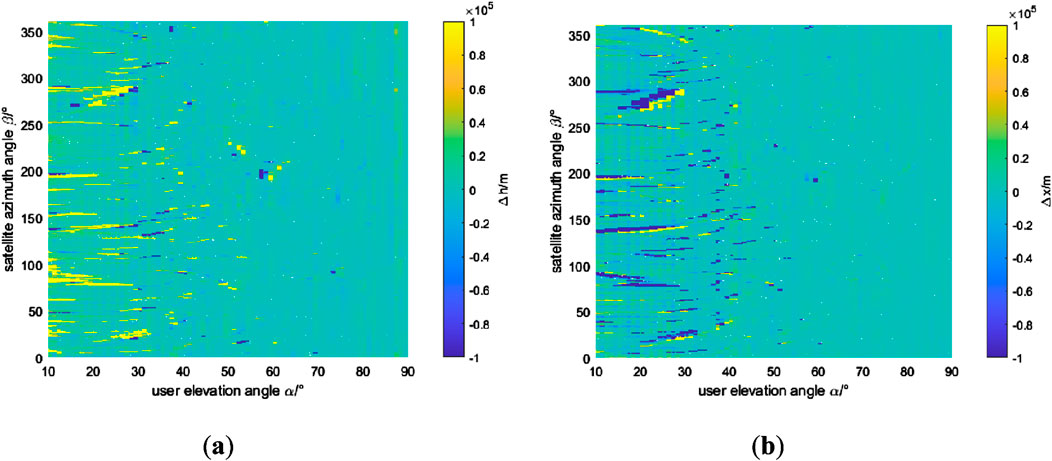
Figure 7. When receiver sensitivity is −160 dB W: (A) User vertical errors in different locations. (B) User horizontal errors in different locations.

It is not difficult to see that when the user is at a low elevation angle, the vertical and horizontal errors deviation of the users are generally large, and the convergence is not good. When the user is at a higher elevation angle, the horizontal and vertical errors of the user significantly decrease.

The following results in Figure 8 are obtained from the statistical analysis of user errors at different user elevation angles.

Figure 8

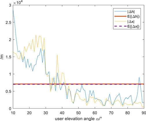
Figure 8. Vertical and horizontal bias of different user elevation angles.

The numerical results of the aforementioned image can be further analyzed. First, by discussing the situation for all users, i.e., users with elevation angles $\alpha ϵ\left[10°,90°\right]$, the overall performance of power positioning can be obtained. Then, by separately discussing the two major parts of low user elevation angles $\alpha ϵ\left[10°,30°\right]$ and high user elevation angles $\alpha ϵ\left[30°,90°\right]$, the positioning and timing performance of users in different elevation angle regions can be obtained as follows in Table 2.

Table 2

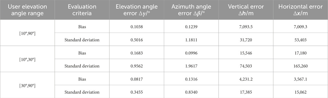
Table 2. Satellite and user error table when receiver sensitivity is −160 dB W.

According to Equation 23, timing errors of the power positioning can be calculated by the difference between the true value and solution value. The timing errors affected by different user locations as follows in Figure 9.

Figure 9

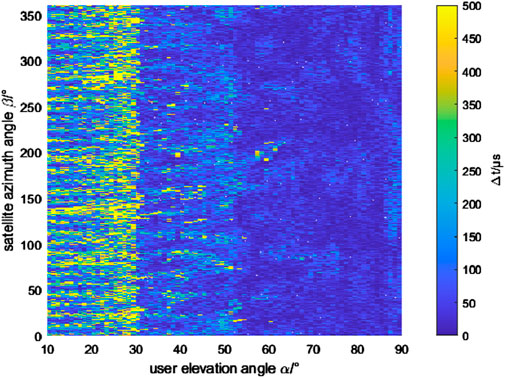
Figure 9. Timing errors of power positioning.

The maximum timing error is 10.1 ms, and the statistical mean is 123 μs. When the user’s elevation angle is below 30°, the average timing error is 305.8 μs; when the user’s elevation angle is above 30°, the average timing error is 62.3 μs. Therefore, power positioning can provide users with microsecond-level timing accuracy.

When the user’s horizontal or vertical difference exceeds the convergence condition of 50 km, the algorithm is judged to diverge, and the availability of power positioning is poor. By statistically analyzing the results for different user elevation angles, the positioning availability can be obtained as shown in Figure 10.

Figure 10

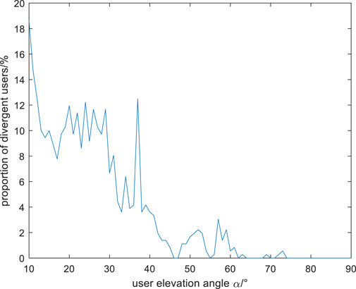
Figure 10. Availability of power positioning.

It can be seen that when the user’s elevation angle is less than 40°, the proportion of divergent users is generally more than 10%, and the availability of power positioning is about 90%; when the elevation angle is higher than 40°, the proportion of divergent users is generally within 5%, and the availability of power positioning is above 95%. In summary, power positioning allows some users, especially those with high elevation angles, to have the potential to achieve better positioning and timing performance.

4.2 Different receiver sensitivity

The simulation is set with a certain receiving power sensitivity threshold. When the received power exceeds this threshold, the power measurements are processed; otherwise, the power value is considered to be significantly affected by noise and is not subjected to least squares iteration processing. Previous simulations were all conducted under the condition of a threshold of −160 dB W, which has high requirements for data quality. In this section, the receiver sensitivity is lowered to −190 dB W to explore the impact of receiving power sensitivity on power positioning.

As with section 4.1, the angle conditions are as the same. However, the receiver sensitivity is set to −190 dB W. Figure 11 illustrates the impact of the user’s elevation angle and azimuth angle on the vertical and horizontal error biases in power positioning.

It can be observed that when the user’s elevation angle is low, for example, below 30°, the receiver with −190 dB W sensitivity exhibits more divergence in power positioning compared to the receiver with −160 dB W sensitivity. This indicates that while increasing the receiver sensitivity makes it easier to receive signals from different beams, the power positioning algorithm becomes more challenging to converge due to noise interference. Therefore, to enable more users to achieve better performance with power positioning, it is necessary to reduce the receiver sensitivity to a certain extent, in order to mitigate the impact of noise on the solution. As with subsection 4.1, by statistically analyzing the error biases for users with different elevation angles, the following results can be obtained.

The resulting error table is as follows.

From Figure 12 and Table 3, it can be seen that the standard deviations of user vertical difference and horizontal difference obtained by the high-sensitivity receiver are comparable to those under low-sensitivity conditions. However, the error biases of satellite elevation angle and satellite azimuth angle have increased by 0.0311° and 0.0789°, respectively, and the biases of user vertical and horizontal errors have increased by 3,556.5 m and 3,859.7 m, respectively. Under low user elevation angles, the biases of vertical difference and horizontal difference have increased by 8,506 m and 10,975 m, respectively, while under high user elevation angles, the biases have increased by 1,790.9 m and 1,343.2 m, respectively. It is not difficult to find that high sensitivity has a very significant impact on users with low elevation angles, while the impact on users with high elevation angles is relatively small.

Figure 11

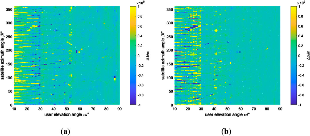
Figure 11. When receiver sensitivity is −190 dB W: (A)User vertical errors in different locations (B) User horizontal errors in different locations.

Figure 12

Figure 12. Vertical and horizontal deviations of different user elevation angles when receiver sensitivity is −190 dB W.

Table 3

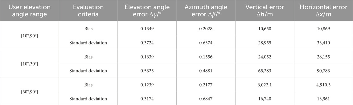
Table 3. Satellite and user error table when receiver sensitivity is −190 dB W.

5 Conclusion

In scenarios where the number of LEO satellites in view is limited, pseudorange and carrier phase positioning are not available, and single-satellite Doppler positioning has poor applicability, ground users can utilize the received power measurements from different beams of LEO satellites to calculate their own position and time, thereby quickly obtaining positioning and timing results. Based on the multi-beam interrogation characteristics of LEO satellites, this paper employs the nearest neighbor algorithm for power matching to obtain convergent initial values and uses the least squares iteration to solve for the user’s horizontal and vertical information. Experimental results show that the nearest neighbor algorithm can achieve initial values for satellite elevation and azimuth angles within 2° when the fingerprint library interval uncertainty is 5°; under the condition of initial values within 2°, the least squares solution can achieve convergence for the vast majority of users (94.5%, 93.2%).

For the least squares algorithm solution, multiple Monte Carlo simulation results indicate that the satellite elevation and azimuth angles, as well as user vertical and horizontal differences obtained from power positioning calculations, follow a normal distribution and have a good normal fitting relationship. There is a significant difference in power positioning results for users at different locations. For a receiver with −160 dB W sensitivity, the statistical error biases for horizontal and vertical positioning are approximately 7,000 m, and the average timing error is 123 μs. Users with low elevation angles (below 30°) generally have error biases higher than the average, at 1,5546 m and 17,180 m respectively, with a timing error of 305.8 μs, and power positioning availability of about 90%. In contrast, users with high elevation angles (above 30°) generally have error biases lower than the average, at 4,231.2 m and 3,567.1 m respectively, with a timing error of 62.3 μs, and availability about 95%. Under high receiver sensitivity at −190 dB W, affected by noise, the average error bias is about 10,000 m, with low elevation angle users being particularly affected, with an average bias worsening to over 20,000 m, and availability worsening to 70%. For high elevation angle users, the average bias only worsens to about 6,000 m, and power positioning availability is basically maintained above 90%.

In summary, the positioning accuracy of low Earth orbit multi-beam power positioning technology is at the kilometer level, and the timing accuracy is at the microsecond level, which can meet users' needs for real-time approximate position and time information.

As the technology of LEO power positioning evolves, future research will delve into the performance of the Least Squares algorithm and the K-Nearest Neighbors algorithm in this domain. By conducting a meticulous analysis of these two algorithms, we aim to uncover their respective advantages in various application scenarios, thereby providing theoretical foundations and technical support for achieving more accurate navigation and timing performance. In this process, our focus will extend beyond the mathematical properties and computational efficiency of the algorithms to encompass their adaptability and flexibility in practical applications. We are confident that through a comprehensive comparison and optimization of these algorithms, we can offer more reliable solutions for LEO power positioning technology in the complex and dynamic environments of its applications. Looking ahead, we anticipate that these research outcomes will propel the advancement of LEO power positioning technology and contribute new momentum to the development of LEO navigation systems.

Data availability statement

The raw data supporting the conclusions of this article will be made available by the authors, without undue reservation.

Author contributions

SG: Data curation, Formal Analysis, Software, Validation, Visualization, Writing–original draft, Writing–review and editing. CM: Data curation, Investigation, Methodology, Supervision, Writing–review and editing. XT: Methodology, Supervision, Writing–review and editing, Investigation, Resources. FW: Methodology, Supervision, Writing–review and editing, Funding acquisition, Software.

Funding

The author(s) declare that financial support was received for the research, authorship, and/or publication of this article. National Natural Science Foundation of China, U20A20193.

Conflict of interest

The authors declare that the research was conducted in the absence of any commercial or financial relationships that could be construed as a potential conflict of interest.

Generative AI statement

The author(s) declare that no Generative AI was used in the creation of this manuscript.

Publisher’s note

All claims expressed in this article are solely those of the authors and do not necessarily represent those of their affiliated organizations, or those of the publisher, the editors and the reviewers. Any product that may be evaluated in this article, or claim that may be made by its manufacturer, is not guaranteed or endorsed by the publisher.

References

1. Yang Y, Yue M, Xia R, Xiaolin J, Bijiao S. Demand and key technology for a LEO constellation as augmentation of satellite navigation systems. Satell Navig (2024) 5(1):1–9. doi:10.1186/s43020-024-00133-w

CrossRef Full Text | Google Scholar

2. Li X, Lu Z, Yuan M, Liu W, Wang F, Yu Y, et al. Tradeoff of code estimation error rate and terminal gain in SCER attack. IEEE Trans Instrumentation Meas (2024) 73:1–12. doi:10.1109/tim.2024.3406807

CrossRef Full Text | Google Scholar

3. Tian R, Cui Z, Zhang S, et al. Overview of the development of navigation augmentation technology based on low-orbit communication constellation. Navigation Positioning and Timing (2021) 8(1):66–81.

Google Scholar

4. Benzerrouk H, Nguyen Q, Fang X, et al. 26th saint petersburg international conference on integrated navigation systems (ICINS). St. Petersburg: IEEE (2019).

Google Scholar

5. Min L, Tengda H, Wenwen L, Qile Z. A review of low earth orbit navigation enhancement technology development. Surv Mapp Geomatics (2024) 49(1):10–9.

Google Scholar

6. Chen L, Kai L, Jin Y, Lin J, Shao H. Design of low earth orbit satellite constellation for regional navigation enhancement. J Univ Electron Sci Technology China (2022) 51(4):522–8.

Google Scholar

7. Zhang X, Hu J, Ren X. New progress in PPP/PPP-RTK and comparison of BeiDou/GNSS PPP positioning performance. Acta Geodaetica et Cartographica Sinica (2020) 49(9):1084–100.

Google Scholar

8. Li X, Zhao Y, Zhang K, Wu J, Zheng H, Zhang W. LEO real-time ambiguity-fixed precise orbit determination with onboard GPS/Galileo observations. GPS Solutions (2024) 28(4):188. doi:10.1007/s10291-024-01729-0

CrossRef Full Text | Google Scholar

9. Hong J, Tu R, Zhang P, Zhang R, Han J, Fan L, et al. GNSS rapid precise point positioning enhanced by low Earth orbit satellites. Satellite Navigation (2023) 4(1):11–3. doi:10.1186/s43020-023-00100-x

CrossRef Full Text | Google Scholar

10. Shi C, Zhang Y, Li Z. Revisiting Doppler positioning performance with LEO satellites. GPS Solutions (2023) 27(3):126. doi:10.1007/s10291-023-01466-w

CrossRef Full Text | Google Scholar

11. Kershner RB, Newton RR. The transit system. J Navigation. (1962) 15(2):129–44. doi:10.1017/s0373463300035943

CrossRef Full Text | Google Scholar

12. Kouba J. A review of geodetic and geodynamic satellite Doppler positioning. Rev Geophys (1983) 21(1):27–40. doi:10.1029/rg021i001p00027

CrossRef Full Text | Google Scholar

13. Yi K, Yi L, Sun C, Chunguo N. Recent developments and prospects of satellite communication. J Commun (2015)(6) 161–76.

Google Scholar

14. Bi J, Wang Y, Cao H, Shi T, Huang L. Supplementary open dataset for WiFi indoor localization based on received signal strength. Satellite Navigation (2022) 3(1):25–15. doi:10.1186/s43020-022-00086-y

CrossRef Full Text | Google Scholar

15. Vincent H, Xiao Z, Semong T, Bai J, Chen H, Jiao L. Achieving reliable intervehicle positioning based on redheffer weighted least squares model under multi-GNSS outages. IEEE Trans Cybernetics (2023) 53(2):1039–50. doi:10.1109/TCYB.2021.3100080

CrossRef Full Text | Google Scholar

16. Xiao Z, Chen Y, Alazab M, Chen H. Trajectory data acquisition via private car positioning based on tightly-coupled GPS/OBD integration in urban environments. IEEE Trans Intell Transportation Syst (2022) 23(7):9680–91. doi:10.1109/tits.2021.3105550

CrossRef Full Text | Google Scholar

17. Kaemarungsi K, Krishnamurthy P. Modeling of indoor positioning systemsbased on location fingerprinting. IEEE INFOCOM (2004) 2:1012–22. doi:10.1109/ACCESS.2018.2817576

CrossRef Full Text | Google Scholar

18. Li J, Gao X, Hu Z, Wang H, Cao T, Yu L. Indoor localization method based on regional division with IFCM. Electronics (2019) 8(5):559. doi:10.3390/electronics8050559

CrossRef Full Text | Google Scholar

19. Kan C, Ding G, Wu Q, et al. Robust relative fingerprinting-based passive source localization via data cleansin. IEEE Access (2018) 6:19295–69.

Google Scholar

20. Feng Y, Minghua J, Jing L, Xiao Q, Ming H, Tao P, et al. Improved AdaBoost-based fingerprint algorithm for WiFi indoor localization. In: 2014 IEEE 7th joint international information technology and artificial intelligence conference (2014). p. 16–9.

Google Scholar

21. Li Y, Zhuang Y, Hu X, Gao Z, Hu J, Chen L, et al. Toward location-enabled IoT (LE-IoT): IoT positioning techniques,error sources, and error mitigation. IEEE Internet Things J (2021) 8(6):4035–62. doi:10.1109/jiot.2020.3019199

CrossRef Full Text | Google Scholar

22. Xie G. Principles of GPS and receiver design. Beijing: Publishing House of Electronics Industry (2022).

Google Scholar

23. Xiao Z, Xiao D, Vincent H, Jiang H, Liu D, Wang D, et al. Toward accurate vehicle state estimation under non-Gaussian noises. IEEE Internet Things J (2019) 6(6):10652–64. doi:10.1109/JIOT.2019.2940412

CrossRef Full Text | Google Scholar

24. GB/T 39399-2020. General specification for BeiDou/global navigation satellite systems (GNSS) geodetic receivers (2020). p. 11–9.

Google Scholar