A two-stage computational approach for stochastic Darcy-forchheimer non-newtonian flows

The study of stochastic non-Newtonian fluid flows in porous media has significant applications in engineering and scientific fields, particularly in geophysical transport, biomedical flows, and industrial filtration systems. This research develops a high-order numerical scheme to solve deterministic and stochastic partial differential equations governing the Darcy–Forchheimer flow of Williamson fluid over a stationary sheet. This study aims to formulate and validate a computationally efficient two-stage method that accurately captures the effects of non-Newtonian behavior, porous media resistance, and stochastic perturbations. The proposed two-stage numerical method integrates a modified time integrator with a second-stage Runge-Kutta scheme, ensuring second-order accuracy in time for deterministic problems. The Euler-Maruyama approach handles Wiener processes for stochastic models, providing robust performance under random fluctuations. A compact sixth-order spatial discretization scheme enhances solution accuracy while maintaining computational efficiency. Numerical experiments, including Stokes’ first problem, demonstrate the superior accuracy and reliability of the proposed method compared to existing second-order Runge-Kutta schemes. The results confirm that the technique effectively captures complex interactions between deterministic and stochastic effects while significantly improving computational efficiency. This study advances numerical techniques for stochastic fluid dynamics, providing a practical framework for modeling and analyzing non-Newtonian fluid flows in porous media with real-world applications in engineering, geophysics, and industrial systems.

1 Introduction

In recent years, the investigation of non-Newtonian fluids has gained considerable interest owing to its complex behaviour, which is crucial in numerous engineering and commercial applications, including petroleum extraction, polymer processing, and biological systems. The Williamson fluid is a non-Newtonian fluid distinguished by its shear-thinning characteristics. The flow characteristics of Williamson fluids, particularly when affected by stochastic factors, pose distinct challenges in modelling and computation because of the nonlinear structure of their governing equations. Numerical strategies are essential for achieving approximate solutions when analytical methods are impractical.

We formulate a resilient two-stage predictor-corrector methodology to tackle the flow’s stochastic characteristics. The predictor phase calculates the solution at an intermediate temporal level, yielding a preliminary estimate, while the corrector phase enhances this solution at the following temporal level. This method facilitates precise time-stepping for the stochastic differential equations that dictate the flow of Williamson fluid, rendering it appropriate for managing the system’s intrinsic uncertainties and unpredictable variations.

Here are the main points of this work:

1. We developed a two-stage numerical scheme for solving deterministic and stochastic partial differential equations with second-order temporal and sixth-order spatial accuracy.

2. We Integrated a compact sixth-order scheme for spatial discretization, enabling efficient handling of spatial gradients in the Darcy–Forchheimer model.

3. In the context of Williamson fluid flow, a thorough examination of the interplay between concentration and temperature gradients, magnetic fields, and the effects of porous media.

4. Comparative analysis of the proposed scheme with the existing second-order Runge-Kutta method, demonstrating superior accuracy in solving the Stokes first problem for the Williamson fluid.

Non-Newtonian fluids exhibit distinct rheological characteristics, defined by their shear-thinning or shear-thickening behaviour. The characteristics mentioned above confer benefits in domains such as fluid transport, mixing, and heat transfer, thereby enhancing the efficiency and performance of various processes. Consequently, these fluids play an essential role in shaping and advancing the domain of modern engineering and industrial methodologies. Recently, a growing body of research has focused on a range of non-Newtonian models, encompassing the viscoelastic system [1], Maxwell system [2], Casson system [3], power-law system [4], Carreau system [5], and Eyring-Powell system [6].

The Williamson model, a significant element in emulsion sheet manufacture, exemplifies one category of such models. This notion is applied in various contexts, including plasma flow, photographic film production, and the understanding of hemodynamics. The shear-thinning properties of the Williamson [7] model in non-Newtonian fluids are well-known. He stressed how this model is crucial for differentiating plastic flow from viscous flow. In addition, he found that this model is just as important in bioengineering, especially for evaluating hemodialysis applications and mass and heat transport in blood arteries. Due to its significance, numerous scholars have dedicated their time and resources to investigating the dynamics of Williamson fluid flow across various conditions, demonstrating the research community’s deep interest and commitment to comprehensively understanding this fluid type. Owing to their importance, these fluids are essential in numerous vital technical and industrial domains. The homotopy analysis method can be used for quantitative analysis [8], in stagnation point flow [9], chemical reactions on a stretching cylinder [10], in porous media [11], with the effects of viscous dissipation and slip velocity [12], with thermal radiation and chemical reaction influences [13], under multiple slip boundary conditions [14], and in nanofluid scenarios with magnetic field effects [15].

According to Williamson, the Williamson fluid model is one of the simplest non-Newtonian models that attempts to capture the behaviour of viscoelastic shear-thinning [16]. A chemical process was used by Krishnamurthy et al. [17] to demonstrate the flow of thermally radiative Williamson fluid on a stretched sheet. Their findings demonstrated a decrease in fluid temperature attributable to the existence of the Williamson parameter. Khan et al. [18] illustrated the effects of slip flow of Williamson nanofluid within a porous media. The surface drag force diminishes as the Williamson fluid parameter increases. Hayat et al. [19] examined a Williamson fluid’s 2D unsteady radiative flow on a porous stretched surface. As the Williamson parameter increases, the fluid velocity decreases. In their investigation of Williamson fluid flow across a stretching sheet, Nadeem et al. [20] discovered that the skin friction coefficient decreases as the Williamson parameter increases. Apply the Keller box method to investigate the MHD flow of Williamson fluid across a stretching sheet, as demonstrated by Salahuddin et al. [21]. Their results suggest that the Williamson fluid parameter decreases fluid velocity. Refs. [22, 23] contain only a few substantial analyses of this subject matter.

Many industrial processes include fluids passing through porous media. Its few uses include drying wood, storing nuclear waste, processing food, refining oil, facilitating drainage, and watering crops. Darcy’s principle analyses flow behaviour under low porosity and small velocity conditions. The Darcy principle didn't work when the Reynolds number amount was more than 1. Forchheimer [24] included the square velocity element in the momentum equation to get around this restriction. Then, for operations involving higher Reynolds numbers, this is referred to as the Forchheimer number. The Darcy–Forchheimer flow of a viscous fluid across a plate was examined by Mukhopadhyay et al. [25] using numerical analysis. The researchers found that lowering the permeability parameter made the fluid colder. The 3D Williamson nanomaterial flow over a Darcy–Forchheimer porous media is shown by Hayat et al. [26]. As the Forchheimer number increases, the surface shear stress decreases. Khan et al. [27] visualized the Darcy–Forchheimer flow of a viscous fluid undergoing heterogeneous-homogeneous chemical processes. The availability of the Darcy number causes a noticeable reduction in the fluid speed, as their data demonstrate. An analysis of the hybrid nanofluid’s Darcy–Forchheimer and slip flow on a revolving disc is carried out by Haider et al. [28]. They demonstrated that a greater estimate of Forchheimer enhances the fluid temperature. Sadiq et al. [29] identified a steady 3D Darcy–Forchheimer flow of carbon nanotubes on a spinning disc in Refs. [30–33], you can find a compilation of significant research on these topics.

A viscous fluid that cannot be compressed and is incompressible is described by the Navier-Stokes equation. Despite the notion that the Navier-Stokes equation is intrinsically deterministic, the fact that certain solutions behave randomly may lead to fresh insights regarding the beginning of turbulence. However, from a purely mathematical point of view, whether solutions to the equation presented above exist and whether they are smooth is still largely unsolved. In the following paragraphs, we will discuss several approaches to analyzing the solutions to the above equation, including a random component.

One famous example of a deterministic equation that conceals unpredictability is the famous Schrödinger equation. Any quantum physics experiment will show some degree of blatant randomness, even though it is not based on mathematical probability theory. Notwithstanding this inexplicable dilemma, Quantum Theory has yielded an impressive suite of control tools, notably the inversion of solutions to classical equations of motion that are (in principle) differentiable and instead display uncertainty. Simulating “dry water” (Von Neumann) only adds another layer of complexity to the already complicated Euler equation.

There seems to be no proof currently that it does not produce singularities [34]. There are other ways to generate randomness, although errors in the initial conditions could also be a source of uncertainty. This calls for applying statistical approaches, such as tracking the evolution of a probability measure in conjunction with the pertinent physical beginning data. See, for instance [35, 36], for examples of how this fits into the statistical approach to turbulence that began in the 19th century. A variety of stochastic diffusion-based Langevin dynamics may account for both equilibrium and non-equilibrium dynamics, as well as Kraichnan’s model in turbulent advection [37]. Nevertheless, the chosen numerical model may include uncertainty (see [38, 39] for further information on this subject in climate modelling).

A popular method for dealing with stochasticity is introducing stochastic partial differential equations by applying random forces to the Navier-Stokes equation. After the revolutionary mathematical work, a deluge of material covers the subject [40]. Even though turbulence usually introduces stochasticity at the Eulerian level, models of the Langevin type that include smooth Lagrangian trajectories and stochastic velocities have been evaluated [41]. D.D. Holm more recently used Lie transfer to introduce stochastic advection [42]. Stochastic partial differential equations describe the resultant motion, and the approach is also Eulerian.

This space cannot accommodate any stochastic methods related to fluid dynamics. A limited number of subjects and their corresponding references have been chosen. It is important to note that several fascinating formulas exist for probabilistic representations. This is a recognized practice in stochastic analysis. A potential application lies in fluid dynamics, where it may be utilized to depict the anticipated values of functionals of stochastic processes as solutions to partial differential equations. Three distinct methodologies are presented: one employs a probabilistic model of the vorticity field, another utilizes branching processes alongside the Fourier transform, and the third implements Lagrangian diffusion processes. For additional information, go to [43–45] accordingly.

This study offers two numerical schemes that can be used to discretize partial differential equations. The scheme is constructed using Taylor series expansion and then implemented to solve the flow problem. The non-Newtonian, incompressible, laminar fluid flow is considered over the flat plate. The governing equations are reduced to dimensionless partial ones rather than ordinary ones. Then, these dimensionless equations are solved using the proposed scheme.

2 Proposed numerical scheme

The proposed scheme is applicable for solving stochastic differential equations; however, a scheme for the deterministic model must be constructed before its construction. The scheme is a bifurcated predictor-corrector framework. The predictor scheme determines the answer at a specified time level, whereas the corrector scheme identifies the solution at the subsequent time level. To propose a scheme, consider the following differential equations.

$\frac{\partial v}{\partial t}=\gamma \frac{{\partial }^{2}v}{\partial y^2}+f\left(v\right)(1)$

where $f\left(v\right)$ represents the nonlinear term in the system, this framework ensures that nonlinear and stochastic effects are managed systematically, avoiding excessive numerical diffusion and providing better stability.

2.1 Step-by-step construction of the scheme

Step 1: Predictor Stage:

Using an explicit exponential integration approach, the predictor stage approximates the solution at an intermediate time step.

${\overline{v}}_i^{n+1}=v_i^n{e}^{0.05\Delta t}+\frac{\left(e^{0.05\Delta t}-1\right)}{0.05}\left[{\left.\frac{\partial v}{\partial t}\right|}_i^n-0.05f_i^n\right](2)$

The symbol $\Delta t$ represents the step size in time. Equation 2 can be called as predictor stage. It uses exponential time integration to enhance stability. Approximates the solution at the next time step before applying corrections. Handles nonlinearity implicitly via the $f\left(v\right)$ term.

Step 2: Corrector Stage:

The corrector stage refines the predicted solution by incorporating further corrections derived using the Taylor series expansion. The corrector stage can be expressed as:

$v_i^{n+1}=a{v}_i^n+b{\overline{v}}_i^{n+1}+c\left(e^{\Delta t}-1\right)\left\{{\left.\frac{\partial \overline{v}}{\partial t}\right|}_i^{n+1}\right\}(3)$

The Taylor series method will determine the parameter in Equation 3.

It is obtained using predictor stage (Equation 2) in Equation 3.

$v_i^{n+1}=a{v}_i^n+b\left[v_i^n{e}^{1.5\Delta t}+\frac{\left(e^{0.05\Delta t}-1\right)}{0.05}\left\{{\left.\frac{\partial v}{\partial t}\right|}_i^n-0.05v_i^n\right\}\right]+c\left(e^{\Delta t}-1\right)\left[{\left.\frac{\partial v}{\partial t}\right|}_i^n{e}^{0.05\Delta t}+\frac{\left(e^{0.05\Delta t}-1\right)}{0.05}\left\{{\left.\frac{{\partial }^{2}v}{\partial t^2}\right|}_i^n-0.05{\left.\frac{\partial v}{\partial t}\right|}_i^n\right\}\right](4)$

The Taylor series expansion for $v_i^{n+1}$ is given as

$v_i^{n+1}=v_i^n+\Delta t{\left.\frac{\partial v}{\partial t}\right|}_i^n+\frac{{\left(\Delta t\right)}^2}{2}{\left.\frac{{\partial }^{2}v}{\partial t^2}\right|}_i^n+O\left({\left(\Delta t\right)}^3\right)(5)$

By inserting the Taylor series expansion (Equation 5) into Equation 4 as

$v_i^n+\Delta t{\left.\frac{\partial v}{\partial t}\right|}_i^n+\frac{{\left(\Delta t\right)}^2}{2}{\left.\frac{{\partial }^{2}v}{\partial t^2}\right|}_i^n=a{v}_i^n+b\left[v_i^n{e}^{0.05\Delta t}+\frac{\left(e^{1.5\Delta t}-1\right)}{1.5}\left\{{\left.\frac{\partial v}{\partial t}\right|}_i^n-0.05v_i^n\right\}\right]+c\left(e^{\Delta t}-1\right)\left[{\left.\frac{\partial v}{\partial t}\right|}_i^n{e}^{0.05\Delta t}+\frac{\left(e^{0.05\Delta t}-1\right)}{0.05}\left\{{\left.\frac{{\partial }^{2}v}{\partial t^2}\right|}_i^n-0.05{\left.\frac{\partial v}{\partial t}\right|}_i^n\right\}\right](6)$

By equating the terms $v_i^n,{\left.\frac{\partial v}{\partial t}\right|}_i^n$ and ${\left.\frac{{\partial }^{2}v}{\partial t^2}\right|}_i^n$ on both sides of Equation 6 it yields

$\left.\begin{array}{c}1=a+b{e}^{0.05\Delta t}-b\left(e^{0.05\Delta t}-1\right)\\ \Delta t=b\frac{\left(e^{0.05\Delta t}-1\right)}{1.5}+c{e}^{0.05\Delta t}\left(e^{\Delta t}-1\right)-c\left(e^{0.05\Delta t}-1\right)\left(e^{\Delta t}-1\right)\\ \frac{{\left(\Delta t\right)}^2}{2}=c\left(e^{\Delta t}-1\right)\frac{\left(e^{0.05\Delta t}-1\right)}{0.05}\end{array}\right\}(7)$

Upon solving Equation 7, the solution can be written as

$\left.\begin{array}{c}a=\frac{1+0.05\Delta t+0.00125{\left(\Delta t\right)}^2-2e^{0.05\Delta t}-0.05\Delta t{e}^{0.05\Delta t}+e^{0.1\Delta t}}{{\left(-1+{\mathrm{e}}^{0.05\Delta t}\right)}^2}\\ b=\frac{0.05\left(-\Delta t-0.025{\left(\Delta t\right)}^2+\Delta t{e}^{0.05\Delta t}\right)}{{\left(-1+{\mathrm{e}}^{0.05\Delta t}\right)}^2}\\ c=\frac{0.025{\left(\Delta t\right)}^2}{\left(-1+e^{0.05\Delta t}\right)\left(-1+e^{\Delta t}\right)}\end{array}\right\}(8)$

These coefficients from Equation 8 are then used in the corrector equation to improve the accuracy of the final solution.

2.1 Space discretization using a compact scheme

The semi-discretized scheme for Equation 1 is written as

${\overline{v}}_i^{n+1}=v_i^n{e}^{0.05\Delta t}+\frac{\left(e^{0.05\Delta t}-1\right)}{0.05}\left\{\gamma {\left.\frac{{\partial }^{2}v}{\partial t^2}\right|}_i^n+f\left(v_i^n\right)-0.05v_i^n\right\}(9)$

$v_i^{n+1}=a{v}_i^n+b{\overline{v}}_i^{n+1}+c\left(e^{\Delta t}-1\right)\left\{\gamma {\left.\frac{{\partial }^2\overline{v}}{\partial t^2}\right|}_i^{n+1}+f\left({\overline{v}}_i^{n+1}\right)\right\}(10)$

Equations 9, 10 are used for time discretization for Equation 1. To discretize space, the variable compact scheme is employed. The compact scheme for Equation 1 can be written as Equations 11, 12

${\overline{v}}_i^{n+1}=v_i^n{e}^{0.05\Delta t}+\frac{\left(e^{0.05\Delta t}-1\right)}{0.05}\left\{C^{-1}D{v}_i^n+f\left(v_i^n\right)-0.05v_i^n\right\}(11)$

$v_i^{n+1}=a{v}_i^n+b{\overline{v}}_i^{n+1}+c\left(e^{\Delta t}-1\right)\left\{C^{-1}D{\overline{v}}_i^{n+1}+f\left({\overline{v}}_i^{n+1}\right)\right\}(12)$

Where $C$ and $D$ are matrices that are constructed from the coefficients of the following equation

${\beta }_1{\left.v^{″}\right|}_{i-1}^n+{\left.v^{″}\right|}_i^n+{\beta }_1{\left.v^{″}\right|}_{i+1}^n=b_{\circ }\frac{\left(v_{i+1}^n-2v_i^n+v_{i-1}^n\right)}{{\left(\Delta y\right)}^2}+b_1\frac{\left(v_{i+2}^n-2v_i^n+v_{i-2}^n\right)}{4{\left(\Delta y\right)}^2}(13)$

Where $b_{\circ }=\frac{4}{3}\left(1-{\beta }_1\right),b_1=\frac{1}{3}\left(10{\beta }_1-1\right)$.

This compact discretization method ensures higher-order spatial accuracy while maintaining computational efficiency. Better resolution of gradients and boundary layer effects.

2.3 Extending the scheme to the stochastic case

The primary objective of this project is to develop a framework for stochastic partial differential equations. To accomplish this, consider the subsequent stochastic partial differential equation.

$\partial v=\left(\gamma \frac{{\partial }^{2}v}{\partial y^2}+f\left(v\right)\right)dt+\sigma vdW(14)$

Where $W$ stands for Wiener process.

The first stage or predictor stage of the proposed scheme for Equation 14 is the same as the first stage of the deterministic model (1). The second stage for stochastic differential Equation 14 can be written as

$v_i^{n+1}=a{v}_i^n+b{\overline{v}}_i^{n+1}+c\left(e^{\Delta t}-1\right)\left\{C^{-1}D{\overline{v}}_i^{n+1}+f\left({\overline{v}}_i^{n+1}\right)\right\}+\sigma v_i^n\Delta W(15)$

Where $\Delta W\sim N\left(0,\Delta t\right)$ represents a Gaussian random variable modelling stochastic fluctuations, the stochastic term adds random perturbations to the velocity evolution.

2.4 Summary of the role of predictor-corrector stages

2.4.1 Handling Nonlinearity

The predictor stage provides a first estimate of the solution, incorporating explicit nonlinear effects. The corrector stage refines the solution using a higher-order correction term, ensuring improved accuracy.

2.4.2 Handling Randomness

The stochastic term $\sigma v_i^n\Delta W$ is incorporated in the corrector stage, ensuring that random perturbations influence the solution dynamically. The scheme maintains numerical stability by properly integrating stochastic terms into the time evolution. This ensures high-order accuracy, stability, and the ability to handle complex stochastic dynamics in Darcy–Forchheimer non-Newtonian flows.

3 Stability analysis

The Von Neumann stability analysis, or Fourier series analysis, is used to assess the stability of finite difference schemes. Using this stability analysis, the difference equation is transformed into trigonometric equations. Further stability conditions are imposed into the trigonometric equations. The analysis provides the exact condition for linear partial differential equations and estimates the actual stability condition for nonlinear partial differential equations. To apply this analysis, consider the following transformations

$C{e}^{iI\psi }={\beta }_1{e}^{\left(i+1\right)I\psi }+e^{iI\psi }+{\beta }_1{e}^{\left(i-1\right)I\psi }(16)$

$D{e}^{iI\psi }=b_{\circ }\frac{\left(e^{\left(i+1\right)I\psi }-2e^{iI\psi }+e^{\left(i-1\right)I\psi }\right)}{{\left(\Delta y\right)}^2}+b_1\frac{\left(e^{\left(i+2\right)I\psi }-2e^{iI\psi }+e^{\left(i-2\right)I\psi }\right)}{4{\left(\Delta y\right)}^2}(17)$

Where $I=\sqrt{-1}$ is an imaginary number.

Applying transformations (Equation 16) and (Equation 17) into the predictor stage of the proposed scheme (Equation 11) yields

${\overline{v}}_i^{n+1}=v_i^n{e}^{0.05\Delta t}+\frac{\left(e^{0.05\Delta t}-1\right)}{0.05}\left\{\gamma \frac{4b_{\circ }\left(\mathit{cos}\psi -1\right)+2b_1\left(\mathit{cos}\psi -1\right)}{2{\left(\Delta y\right)}^2\left(2{\beta }_1\cos \psi +1\right)}-0.05\right\}{v}_i^n(18)$

Re-write Equation 18 as

${\overline{v}}_i^{n+1}=\delta v_i^n(19)$

Where $\delta =e^{0.05\Delta t}+\frac{\left(e^{0.05\Delta t}-1\right)}{0.05}\left\{\gamma \frac{4b_{\circ }\left(\mathit{cos}\psi -1\right)+2b_1\left(\mathit{cos}\psi -1\right)}{2{\left(\Delta y\right)}^2\left(2{\beta }_1\cos \psi +1\right)}-0.05\right\}$

Incorporating transformation (Equations 16, 17) into the second corrector stage of the scheme (Equation 15) gives using $f=0$.

$v_i^{n+1}=a{v}_i^n+b{\overline{v}}_i^{n+1}+c\left(e^{\Delta t}-1\right)\left\{\gamma \left(\frac{4b_{\circ }\left(\mathit{cos}\psi -1\right)+2b_1\left(\mathit{cos}\psi -1\right)}{2{\left(\Delta y\right)}^2\left(2{\beta }_1\cos \psi +1\right)}\right)\right\}{\overline{v}}_i^{n+1}+\sigma v_i^n\Delta W(20)$

By using the first stage (Equation 19) in the second stage (Equation 20) it yields

$v_i^{n+1}=a{v}_i^n+b\delta v_i^n+c\left(e^{\Delta t}-1\right)\left\{\gamma \left(\frac{4b_{\circ }\left(\mathit{cos}\psi -1\right)+2b_1\left(\mathit{cos}\psi -1\right)}{2{\left(\Delta y\right)}^2\left(2{\beta }_1\cos \psi +1\right)}\right)\delta v_i^n\right\}+\sigma v_i^n\Delta W(21)$

Re-write Equation 21 as

$v_i^{n+1}={\delta }_1{v}_i^n+\sigma v_i^n\Delta W(22)$

Where ${\delta }_1=a+b\delta +c\left(e^{\Delta t}-1\right)\left\{\gamma \left(\frac{4b_{\circ }\left(\mathit{cos}\psi -1\right)+2b_1\left(\mathit{cos}\psi -1\right)}{2{\left(\Delta y\right)}^2\left(2{\beta }_1\cos \psi +1\right)}\right)\right\}\delta$ in Equation 22

The amplification factor can be expressed as

$\frac{v_i^{n+1}}{v_i^n}={\delta }_1+\sigma \Delta W(23)$

By using the expected value of the square of the amplification factor, Equation 23 is written as

$E{\left|\frac{v_i^{n+1}}{v_i^n}\right|}^2\le 2E{\left|{\delta }_1\right|}^2+2{\sigma }^{2}E{\left|\Delta W\right|}^2(24)$

If ${\left|{\delta }_1\right|}^2<1$ and let, $2{\sigma }^2=\lambda$ then inequality (Equation 24) is stated as

$E{\left|\frac{v_i^{n+1}}{v_i^n}\right|}^2\le 1+\lambda \Delta t(25)$

The scheme will remain stable in the mean square sense if it meets conditions (Equation 25); otherwise, the solution will be unstable.

Theorem 1. The proposed time and compact scheme in space are consistent in the mean square sense.

Proof: Let $P$ be the smooth function

$L{\left(P\right)}_i^n=P\left(\left(n+1\right)\Delta t,i\Delta x\right)-P\left(n\Delta t,i\Delta x\right)-\gamma {\int }_{n\Delta t}^{\left(n+1\right)\Delta t}{P}_{yy}\left(\mathrm{s},i\Delta x\right)dS-\sigma {\int }_{n\Delta t}^{\left(n+1\right)\Delta t}P\left(s,i\Delta x\right)dW\left(s\right)(26)$

$\begin{array}{c}{L}_i^{n}P=P\left(\left(n+1\right)\Delta t,i\Delta x\right)-P\left(n\Delta t,i\Delta x\right)-b\frac{\left(e^{0.05\Delta t}-1\right)}{0.05}{C}^{-1}DP\left(n\Delta t,i\Delta x\right)\hfill \\ +c\left(e^{\Delta t}-1\right)C^{-1}D\overline{P}\left(\left(n+1\right)\Delta t,i\Delta x\right)-\sigma P\left(n\Delta t,i\Delta x\right)\left(W\left(\left(n+1\right)\Delta t\right)-W\left(n\Delta t\right)\right)\end{array}(27)$

Where $\overline{P}\left(\left(n+1\right)\Delta t,i\Delta x\right)=P\left(n\Delta t,i\Delta x\right)e^{0.05\Delta t}+\frac{\left(e^{0.05\Delta t}-1\right)}{0.05}$$\{C^{-1}DP\left(n\Delta t,i\Delta x\right)-0.05P(n\Delta t,i\Delta \left.x)\right\}$

By subtracting Equation 27 from Equation 26 and then applying the absolute value of the square of difference it yields

$\begin{array}{c}E{\left|L\left(P_i^n\right)-L_i^{n}P\right|}^2=E\left|\right.-\gamma {\int }_{n\Delta t}^{\left(n+1\right)\Delta t}{P}_{yy}\left(\mathrm{s},i\Delta x\right)dS-\sigma {\int }_{n\Delta t}^{\left(n+1\right)\Delta t}P\left(\mathrm{s},i\Delta x\right)dW\left(s\right)\hfill \\ +b\frac{\left(e^{0.05\Delta t}-1\right)}{0.05}{C}^{-1}DP\left(n\Delta t,i\Delta x\right)+c\left(e^{\Delta t}-1\right)C^{-1}D\overline{P}\left(\left(n+1\right)\Delta t,i\Delta x\right)\\ +\sigma P\left(n\Delta t,i\Delta x\right)\left(W\left(\left(n+1\right)\Delta t\right)\right){\left.\right|}^2\hfill \\ \end{array}(28)$

Re-write Equation 28 as

$\begin{array}{c}E{\left|L\left(P_i^n\right)-L_i^{n}P\right|}^2\le 2\gamma E\left|\right.{\int }_{n\Delta t}^{\left(n+1\right)\Delta t}{P}_{yy}\left(\mathrm{s},i\Delta x\right)dS-b\frac{\left(e^{0.05\Delta t}-1\right)}{0.05}{C}^{-1}DP\left(n\Delta t,i\Delta x\right)\hfill \\ +c\left(e^{\Delta t}-1\right)C^{-1}D\overline{P}\left(\left(n+1\right)\Delta t,i\Delta x\right){\left.\right|}^2+2{\sigma }^{2}E\left|\right.{\int }_{n\Delta t}^{\left(n+1\right)\Delta t}P\left(\mathrm{s},i\Delta x\right)dW\left(s\right)\\ -P\left(n\Delta t,i\Delta x\right)\left(W\left(\left(n+1\right)\Delta t\right)-W\left(n\Delta t\right)\right){\left.\right|}^2\end{array}(29)$

Now consider the inequality

$E{\left|{\int }_{t_{\circ }}^{t}f\left(s,W\right)dW\left(s\right)\right|}^{2m}\le {\left(t-t_{\circ }\right)}^{m-1}{\left[m\left(2m-1\right)\right]}^m{\int }_{t_{\circ }}^{t}E\left[{\left|f\left(s,W\right)\right|}^{2m}\right]ds(30)$

The use of inequality (Equation 30) in inequality (Equation 29) yields

$\begin{array}{c}E{\left|L\left(P_i^n\right)-L_i^{n}P\right|}^2\le 2\gamma E\left|\right.{\int }_{n\Delta t}^{\left(n+1\right)\Delta t}{P}_{yy}\left(\mathrm{s},i\Delta x\right)dS-b\frac{\left(e^{0.05\Delta t}-1\right)}{0.05}{C}^{-1}DP\left(n\Delta t,i\Delta x\right)\hfill \\ +c\left(e^{\Delta t}-1\right)C^{-1}D\overline{P}\left(\left(n+1\right)\Delta t,i\Delta x\right){\left.\right|}^2\\ +2{\sigma }^2\Delta t{\int }_{n\Delta t}^{\left(n+1\right)\Delta t}E\left[{\left|P\left(\mathrm{s},i\Delta x\right)-P\left(n\Delta t,i\Delta x\right)\right|}^2\right]\text{dS}\end{array}(31)$

Upon applying the $limit$ in Equation 31 as $\Delta x\to 0,\Delta t\to 0,t=\left(n+1\right)\Delta t,\left(n\Delta t,i\Delta x\right)\to \left(t,x\right),$ then the mean square error tends to zero.i.e.

$E{\left|L\left(P_i^n\right)-L_i^{n}P\right|}^2\to 0(32)$

Thus, the proposed scheme in time and compact spatial discretization is consistent in the mean square sense proved by Equation 32.

Here, we provide a comparative summary highlighting the stability criteria of our proposed scheme versus alternative methods. Below, we outline a summary of Table 1 comparing the stability characteristics of the proposed method against existing numerical schemes.

The Von Neumann stability analysis is applied to derive the stability condition. The stochastic nature of the problem requires the scheme to be stable in the mean-square sense. The derived stability condition is: $E{\left|\frac{v_i^{n+1}}{v_i^n}\right|}^2\le 1+\lambda \Delta t$. This ensures the numerical scheme remains bounded over time, preventing error amplification.

Table 1 effectively compares the stability criteria, stochastic effects, accuracy, and efficiency of the proposed method versus alternative approaches. The proposed scheme ensures stability in stochastic problems and offers superior accuracy and computational efficiency.

Table 1

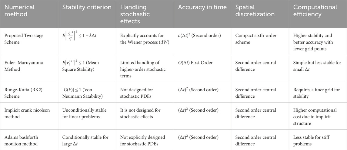
Table 1. Comparison of stability criteria with alternative methods.

4 Problem formulation

Examine a laminar, unstable, incompressible Williamson fluid above a fixed plate. The fluid flow is propelled by temperature and concentration gradients. Let $x*$-axis is taken perpendicular along the plate and $y*$- axis is taken horizontally. Suppose the ambient temperature and concentration are less than those at the plate. At $t*=0$ the temperature and concentration are represented by $T_{\infty }$ and $C_{\infty }$ respectively. After $t*>0$ both temperature and concentration become $T_{\infty }$ and $C_{\infty }$ plus some periodic functions. Figure 1 illustrates the physical and mathematical configuration of the problem involving non-Newtonian Williamson fluid flow over a stationary vertical sheet under the influence of Darcy–Forchheimer porous medium effects, thermal diffusion, and solutal diffusion. The $x*$-axis represents the horizontal direction along the sheet. The $y*$-axis represents the normal direction (perpendicular) to the sheet. The coordinate system is essential in defining velocity components, boundary layer thicknesses, and external forces acting on the flow. The figure depicts three different boundary layers: The momentum boundary layer (Black Curve) Represents the region where the velocity of the fluid gradually transitions from zero (no slip at the wall) to the free-stream velocity. Thermal boundary layer (Orange Curve): Shows the temperature distribution within the fluid, where heat transfer occurs from the wall to the fluid. Concentration boundary layer (Purple Curve): Indicates the distribution of solute concentration in the fluid, where mass transfer occurs due to concentration gradients. Gravity ($\left.g\right)$: Acts downward, influencing the buoyancy-driven (natural convection) effects in the fluid flow. Magnetic Field $B_{\circ }$: Represents an applied transverse magnetic field, which affects the flow characteristics due to the magnetohydrodynamics (MHD) effect. Porous Medium Effects: The presence of Darcy–Forchheimer drag forces affects the momentum balance, introducing resistance to the fluid flow. At the wall (y* = 0): The velocity $u*$ is zero due to the no-slip condition, and the temperature $T$ and concentration $C$ are prescribed. The expressions: $u*=0,T=T_w+{ϵ}_1\left(T_w-T_{\infty }\right)\cos \left(wt\right),C=C_w+{ϵ}_1\left(C_w-C_{\infty }\right)\cos \left(wt\right)$ indicate that temperature and concentration vary periodically over time due to oscillations in wall properties. Far from the wall (as $y*\to \infty$): The velocity approaches zero, and temperature and concentration reach their respective free-stream values $T_{\infty }$ and $C_{\infty }$. Considering the effect of the Darcy Forchheimer model, the governing equations of the flow can be expressed as [46]

$\frac{\partial u^{*}}{\partial t^{*}}=\nu \frac{{\partial }^2{u}^{*}}{\partial {y^{*}}^2}+\sqrt{2}\nu \mathrm{\Gamma }\frac{{\partial }^2{u}^{*}}{\partial {y^{*}}^2}\frac{\mathrm{\partial }{u}^{*}}{\partial y^{*}}-\overline{b}{u^{*}}^2+g{\beta }_T\left(T-T_{\infty }\right)+g{\beta }_c\left(C-C_{\infty }\right)+\frac{\sigma B_{\circ }^2}{\rho }{u}^{*}-\frac{\nu }{k_p}{u}^{*}(33)$

$\frac{\partial T}{\partial t^{*}}=\alpha \frac{{\partial }^{2}T}{\partial {y^{*}}^2}+q^{‴}(34)$

$\frac{\partial C}{\partial t^{*}}=D\frac{{\partial }^{2}C}{\partial {y^{*}}^2}-k_c\left(C-C_{\infty }\right)(35)$

Figure 1

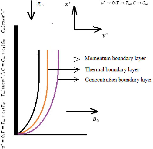
Figure 1. Geometry of the problem.

Here is the explanation of each equation used in problem formulation:

Momentum (Velocity) Equation 33: $\frac{\partial u^{*}}{\partial t^{*}}$: represents the time-dependent change in velocity. $\nu \frac{{\partial }^{2}u*}{\partial {y^{*}}^2}$: represents the viscous diffusion term (Laplacian of velocity). $\sqrt{2}\nu \mathrm{\Gamma }\frac{{\partial }^{2}u*}{\partial {y^{*}}^2}\frac{\mathrm{\partial }u*}{\partial y^{*}}$: Accounts for the non-Newtonian Williamson fluid effects, where $\mathrm{\Gamma }$ is the Williamson parameter. $\overline{b}{u*}^2$: represents the Forchheimer drag force, a correction to the Darcy resistance term. $g{\beta }_T\left(T-T_{\infty }\right)$: represents buoyancy forces due to thermal variations. $g{\beta }_c\left(C-C_{\infty }\right)$: represents buoyancy forces due to concentration variations. $\frac{\sigma B_{\circ }^2}{\rho }u*$: represents the magnetohydrodynamic (MHD) Lorentz force, which opposes the flow. $-\frac{\nu }{k_p}u*$: represents Darcy’s resistance in the porous medium.

Energy (Heat Transfer) Equation 34: $\frac{\partial T}{\partial t^{*}}$: represents the time-dependent change in temperature. $\alpha \frac{{\partial }^{2}T}{\partial {y^{*}}^2}$: represents heat conduction (thermal diffusion). $q^{‴}=\frac{k{u}_R}{\rho x^{*}\nu c_p}\left(A*u\left(T_w-T_{\infty }\right)+B^{*}\left(T-T_{\infty }\right)\right):$ represents the internal heat generation where $A*$ and $B^{*}$ are dimensionless coefficients of space and temperature-dependent terms, respectively.

Concentration (Mass Diffusion) Equation 35: $\frac{\partial C}{\partial t^{*}}$: represents the time-dependent change in concentration. $D\frac{{\partial }^{2}C}{\partial {y^{*}}^2}$: represents mass diffusion. $-k_c\left(C-C_{\infty }\right)$: Represents a first-order chemical reaction, where reactants are consumed over time.

Subject to initial and boundary conditions

$\left.\begin{array}{l}\begin{array}{l}{u}^{*}=0,T=T_{\infty },C=C_{\infty }when{t}^{*}=0\\ u^{*}=0,T=T_{\infty }+{ϵ}_1\left(T_w-T_{\infty }\right)\mathit{cos}{w}^{*}{t}^{*},\\ C=C_{\infty }+{ϵ}_1\left(C_w-C_{\infty }\right)\mathit{cos}{w}^{*}{t}^{*}when{y}^{*}=0\end{array}\\ u^{*}\to 0,T\to T_{\infty },C\to C_{\infty }when{y}^{*}\to \infty \end{array}\right\}(36)$

Let $B_{\circ }$ is the strength of the magnetic field applied transversely to the plate. Now, using the transformations (Equation 36). By introducing non-dimensional variables, the governing equations are transformed into a more convenient form for numerical analysis:

4.1 Non-dimensional variables

$\left.y=\frac{y^{*}}{L_R},u=\frac{u^{*}}{u_R},w=t_R{w}^{*},t=\frac{t^{*}}{t_R},\theta =\frac{T-T_{\infty }}{T_w-T_{\infty }},\varphi =\frac{C-C_{\infty }}{C_w-C_{\infty }}\right\}(37)$

where $u_R={\left(\nu g{\beta }_T\Delta T\right)}^{\frac{1}{3}}$: Characteristic velocity scale, $L_R={\left(\frac{g{\beta }_T\Delta T}{{\nu }^2}\right)}^{-\frac{1}{3}}$: Characteristic length scale and $t_R={\left(g{\beta }_T\Delta T\right)}^{-\frac{2}{3}}{\nu }^{\frac{1}{3}}$: Characteristic time scale as mentioned in Equation 37.

The governing Equations 33–36 are reduce to Equations 38–40

$\frac{\partial u}{\partial t}=\frac{{\partial }^{2}u}{\partial y^2}+W_e\frac{{\partial }^{2}u}{\partial y^2}\frac{\partial u}{\partial y}-\left(M+\frac{1}{D_a}\right)u-F_s{u}^2+\theta +NC(38)$

$\frac{\partial \theta }{\partial t}=\frac{1}{P_r}\frac{{\partial }^2\theta }{\partial y^2}+\frac{ϵ}{P_r}\left(A^{*}u+B^{*}\theta \right)(39)$

$\frac{\partial \varphi }{\partial t}=\frac{1}{S_c}\frac{{\partial }^2\varphi }{\partial y^2}-\gamma \varphi (40)$

subject to the dimensionless initial and boundary conditions

$\left.\begin{array}{c}u=0,\theta =0,\varphi =0fort=0\\ u=0,\theta ={\epsilon }_{1}coswt,\varphi ={\epsilon }_{1}coswtfory=0\\ u\to 0,\theta \to 0,\varphi \to 0fory\to \infty \end{array}\right\}(41)$

Where in Equation 41 $N$, $D_a$, $M$, $P_r$, $W_e$, $S_c$, $ϵ$, $F_S$ and $\gamma$ are given as

$\begin{array}{ll}\hfill & \hfill {N=\frac{{\beta }_c\left(C_w-C_{\infty }\right)}{{\beta }_T\left(T_w-T_{\infty }\right)},D}_a=\frac{k}{\nu t_R},M=\frac{t_R\sigma B_{\circ }^2}{\rho },P_r=\frac{\nu k}{\rho c_p},\\ \hfill & \hfill W_e=\frac{\mathrm{\Gamma }{\mathrm{u}}_{\mathrm{R}}}{L_R},ϵ=\frac{t_R{u}_R}{x^{*}},F_s=\overline{b}{u}_R{t}_R,\gamma =t_R{k}_c\end{array}$

The dimensionless local Nusselt and Sherwood numbers are given as Equation 42

$\left.\begin{array}{c}{N}_{u_L}=-{\left.\frac{\partial \theta }{\partial y}\right|}_{y=0}\\ S_{h_L}=-{\left.\frac{\partial \varphi }{\partial y}\right|}_{y=0}\end{array}\right\}(42)$

These describe the rate of heat and mass transfer at the surface.

The stochastic model is written as Equations 43–45

$\partial u=\left(\frac{{\partial }^{2}u}{\partial y^2}+W_e\frac{{\partial }^{2}u}{\partial y^2}\frac{\partial u}{\partial y}-\left(M+\frac{1}{D_a}\right)u-F_s{u}^2+\theta +NC\right)dt+{\sigma }_{1}u\Delta W(43)$

$\partial \theta =\left(\frac{1}{P_r}\frac{{\partial }^2\theta }{\partial y^2}+\frac{ϵ}{P_r}\left(A^{*}u+B^{*}\theta \right)\right)dt+{\sigma }_2\theta \Delta W(44)$

$\partial \varphi =\left(\frac{1}{S_c}\frac{{\partial }^2\varphi }{\partial y^2}-\gamma \varphi \right)dt+{\sigma }_3\varphi \Delta W(45)$

Subject to the same initial and boundary conditions for the deterministic model.

5 Results and discussions

We present a detailed simulation study with the following objectives:

5.1 Demonstrate the accuracy and efficiency of the proposed two-stage computational approach

The proposed computational approach is validated for both deterministic and stochastic models. For deterministic problems, the method exhibits second-order accuracy, while it demonstrates improved accuracy for stochastic differential equations compared to the conventional Euler-Maruyama method. The Euler-Maruyama scheme is an adaptation of the classical Euler method that incorporates the Wiener process term, efficiently managed in our approach through a two-stage process. The first phase involves modifying the exponential integrator, while the second phase employs the Runge-Kutta method. The results confirm that the scheme effectively captures deterministic and stochastic effects, ensuring numerical stability in the mean-square sense for stochastic diffusion equations.

5.2 Demonstrate stability and performance of the proposed scheme

The stability of the proposed scheme is verified for the scalar stochastic diffusion equation. Unlike traditional approaches, the scheme preserves consistency in the mean and does not require linearization to address nonlinear differential equations. The explicit nature of the scheme ensures efficient computation by solving the differential equations in two distinct phases: the first stage excludes the Wiener process, while the second stage incorporates it. Numerical simulations confirm the scheme’s robustness in handling nonlinear Darcy–Forchheimer flows and effectively capturing oscillatory boundary conditions.

5.3 Investigate the impact of key physical parameters on the velocity, temperature, and concentration profiles

5.3.1 Effect of the Weissenberg number ${\mathit{W}}_{\mathit{e}}$ on velocity

Figure 2 illustrates the impact of the Weissenberg number $W_e$ on the velocity profile of a non-Newtonian Williamson fluid in a porous medium. The Weissenberg number is a dimensionless quantity that characterizes the elastic effects of a fluid, representing the ratio of elastic forces to viscous forces. The graph shows velocity variations for three different values of $W_e$ $\left(0.1,0.5,0.9\right)$ while keeping other parameters constant: $Fs=0.1,Da=7,N=0.1,M=0.1,A^{*}=0.1,B^{*}=0.1,\mathit{Pr}=0.9,\gamma =0.1,Sc=0.9,$$\epsilon =0.1,{\epsilon }_1=0.1$. The velocity initially increases near the boundary due to the no-slip condition at the wall. A peak velocity is observed at a certain distance from the wall, gradually decreasing and asymptotically approaching zero at larger distances. Higher Weissenberg numbers lead to a decrease in the overall velocity. The solid blue line represents $W_e=0.1$, the dashed line represents $W_e=0.5$, and the dotted line represents $W_e=0.9$. As $W_e$ increase, the peak velocity decreases due to the increase in fluid elasticity. A higher $W_e$ implies a longer relaxation time for the fluid, making it more resistant to deformation and flow. This causes the velocity to drop. The flow decelerates faster for higher $W_e$, leading to lower fluid motion further from the boundary. Since the Williamson fluid exhibits shear-thinning behavior, the increase in Weissenberg number reduces the velocity as the fluid becomes more resistant to flow. A lower Weissenberg number ($W_e=0.1$) means the fluid behaves closer to Newtonian behavior, allowing higher velocity. For higher $W_e=0.9$, the elastic nature of the fluid dominates, leading to stronger internal resistance and lower velocity.

Figure 2

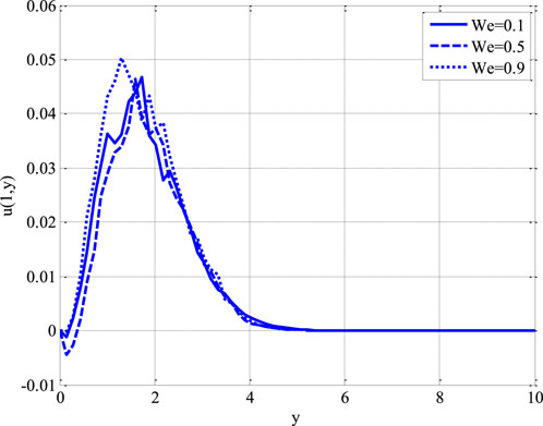
Figure 2. Effect of weissenberg number on velocity profile using $Fs=0.1,Da=7,N=0.1,M=0.1,$$A^{*}=0.1,B^{*}=0.1,\mathit{Pr}=0.9,\gamma =0.1,$$Sc=0.9,\epsilon =0.1,{\epsilon }_1=0.1$.

5.3.2 Effect of the magnetic parameter $\mathit{M}$ on velocity

Figure 3 illustrates the impact of the magnetic field parameter $M$ on the velocity profile of a non-Newtonian Williamson fluid in a porous medium. The analysis is performed while keeping other parameters constant: $Fs=0.1,Da=7,N=0.1,We=0.1,A^{*}=0.1,B^{*}=0.1,\mathit{Pr}=0.9,\gamma =0.9,Sc=0.9,$$\epsilon =0.1,{\sigma }_1=1,{\sigma }_2=1,{\sigma }_3=1$. The velocity starts from zero at the wall due to the no-slip condition. It increases sharply, reaches a peak, and then gradually declines, eventually approaching zero at larger distances. Higher values of $M$ lead to a decrease in velocity across the profile. The solid line $M=0.1$ represents the case with a weak magnetic field. The dashed line $M=0.5$ and dotted line $M=0.9$ show results for increasing magnetic effects. As $M$ increases, the peak velocity decreases, and the velocity profile declines more rapidly. The presence of a magnetic field introduces a Lorentz force, which acts as a resistive force (opposing the fluid motion). As $M$ increases, the magnitude of the Lorentz force increases, which results in greater resistance to fluid movement.

Figure 3

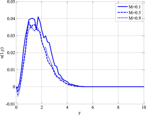
Figure 3. Effect of magnetic parameter on velocity profile using $Fs=0.1,Da=7,N=0.1,We=0.1,$$A^{*}=0.1,B^{*}=0.1,\mathit{Pr}=0.9,\gamma =0.9,$$Sc=0.9,\epsilon =0.1,{\sigma }_1=1,{\sigma }_2=1,{\sigma }_3=1$

5.3.3 Effect of Forchheimer Number ${\mathit{F}}_{\mathit{s}}$ on Velocity Profile

Figure 4 illustrates the effect of the Forchheimer number $F_s$ on the velocity profile of a non-Newtonian Williamson fluid in a porous medium. The analysis is conducted while keeping other parameters constant: $M=0.1,Da=7,N=0.1,We=0.1,A*=0.1,B^{*}=0.1,\mathit{Pr}=0.9,\gamma =0.9,Sc=0.9,$$\epsilon =0.1,{\sigma }_1=1,{\sigma }_2=1,{\sigma }_3=1$. The velocity starts from zero at the wall due to the no-slip condition. It increases sharply, reaches a peak velocity, and then gradually declines, approaching zero at larger distances. Higher values of $F_s$ lead to a decrease in velocity throughout the profile. The solid line $F_s=0.1$ represents the case with a lower Forchheimer number. The dashed line $F_s=0.5$ and dotted line $F_s=0.9$ shows the velocity profiles as Fs increases. As $F_s$ increases, the peak velocity decreases, and the velocity profile shifts downward. The Forchheimer number $F_s$ represents the effect of inertial drag forces in a porous medium. In classical Darcy’s law, the flow resistance in a porous medium is proportional to velocity, but at higher velocities, inertial effects become significant, leading to the nonlinear Forchheimer drag term.

Figure 4

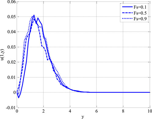
Figure 4. Effect of Forchheimer number on velocity profile using $M=0.1,Da=7,N=0.1,We=0.1,$$A^{*}=0.1,B^{*}=0.1,\mathit{Pr}=0.9,\gamma =0.9,$$Sc=0.9,\epsilon =0.1,{\sigma }_1=1,{\sigma }_2=1,{\sigma }_3=1$.

5.3.4 Effect of heat source coefficient on temperature

Figure 5 illustrates the effect of the coefficient of the space-dependent term in the heat source $\mathrm{A}*$ on the temperature profile of a non-Newtonian Williamson fluid in a porous medium. The analysis is conducted while keeping other parameters constant: $\mathrm{M}=0.1,\text{Da}=7,\mathrm{N}=0.1,{\mathrm{W}}_{\mathrm{e}}=0.1,{\mathrm{F}}_{\mathrm{s}}=0.1,{\mathrm{B}}^{*}=0.1,{\mathrm{P}}_{\mathrm{r}}=0.9,\mathrm{\gamma }=0.9,$$\text{Sc}=0.9,\mathrm{\epsilon }=0.1,{\mathrm{\sigma }}_1=0,{\mathrm{\sigma }}_2=0,{\mathrm{\sigma }}_3=0$. The temperature starts from a minimum value at the boundary. It increases rapidly to a peak temperature and then gradually decreases, approaching an equilibrium state further from the wall. Higher values of $A*$ lead to an increase in the overall temperature profile. The solid line $\mathrm{A}*=0.1$ represents a lower heat source intensity. The dashed line $\mathrm{A}*=3.0$ and dotted line $A*=5.0$ shows an increase in $A*$. As $A*$ increases, the maximum temperature increases, and the temperature profile rises at all points. $A*$ represents the intensity of space-dependent heat generation in the fluid.

Figure 5

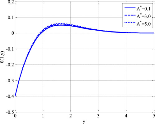
Figure 5. Effect of coefficient of space dependent term in heat source on temperature profile using $M=0.1,Da=7,N=0.1,We=0.1,$$Fs=0.1,B^{*}=0.1,\mathit{Pr}=0.9,\gamma =0.9,$$Sc=0.9,\epsilon =0.1,{\sigma }_1=0,{\sigma }_2=0,{\sigma }_3=0$.

5.3.5 Effect of reaction rate parameter $\gamma$ on concentration

Figure 6 illustrates the effect of the reaction rate parameter $\gamma$ on the concentration profile of a non-Newtonian Williamson fluid in a porous medium. The study is conducted while keeping the following parameters constant: $M=0.1,Da=7,N=0.1,We=0.1,Fs=0.1,B^{*}=0.1,\mathit{Pr}=0.9,A^{*}=0.9,Sc=0.9,$$\epsilon =0.1,{\sigma }_1=0,{\sigma }_2=0,{\sigma }_3=0$. The concentration starts from a low value at the boundary and increases rapidly to a peak concentration before gradually declining to an equilibrium value. Higher values of $\gamma$ lead to a reduction in the overall concentration profile, meaning that the concentration distribution becomes flatter for higher reaction rates. The solid line $\gamma =0.1$ represents a lower reaction rate. The dashed line $\gamma =0.5$ and dotted line $\gamma =0.9$ represent increasing reaction rates. As $\gamma$ increases, the peak concentration decreases, and the concentration profile flattens. The reaction rate parameter $\gamma$ represents the rate at which chemical reactions consume or transform species in the concentration field. When $\gamma$ is small, the chemical reaction is slow, allowing the concentration to build up before gradually diffusing.

Figure 6

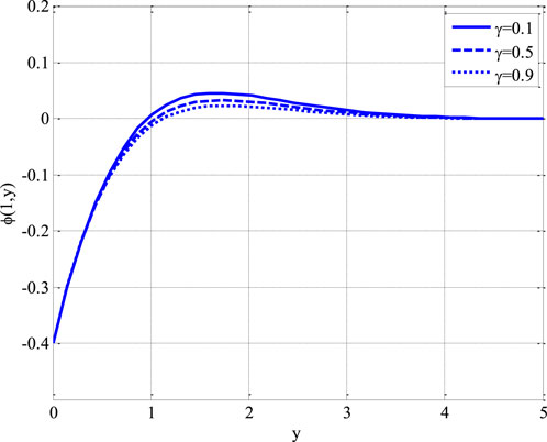
Figure 6. Effect of reaction rate parameter on concentration profile using $M=0.1,Da=7,N=0.1,We=0.1,$$Fs=0.1,B^{*}=0.1,\mathit{Pr}=0.9,A^{*}=0.9,$$Sc=0.9,\epsilon =0.1,{\sigma }_1=0,{\sigma }_2=0,{\sigma }_3=0$.

5.4 Study the effect of key parameters on local nusselt and sherwood numbers

5.4.1 Impact of Prandtl number and heat source coefficient on the local Nusselt number

Figure 6 illustrates the effect of the Prandtl number ${\mathrm{P}}_{\mathrm{r}}$ and the coefficient of the temperature-dependent term in the heat source $B^{*}$ on the local Nusselt number $N_{u_L}$ in a non-Newtonian Williamson fluid flow through a porous medium. (Figure 7) The analysis is conducted while keeping the following parameters constant: $M=0.1,Da=7,N=0.1,We=0.1,Fs=0.1,\gamma =0.9,A^{*}=0.1,Sc=0.9,\epsilon =0.1,$${\sigma }_1=0,{\sigma }_2=0,{\sigma }_3=0$. The Nusselt number $N_{u_L}$ decreases with an increase in the distance from the wall. The profiles remain almost identical for different values of $B^{*}$, with a slight decline in heat transfer rate as $B^{*}$ increases. The solid line $B^{*}=0.1$ represents a lower coefficient of the temperature-dependent heat source. The dashed line $B^{*}=3.0$ and dotted line $B^{*}=5.0$ represent increasing $B^{*}$. As $B^{*}$ increases, the Nusselt number $N_{u_L}$ decreases slightly, indicating a reduction in heat transfer efficiency. The local Nusselt number $N_{u_L}$ represents the convective heat transfer rate relative to conductive heat transfer. The Prandtl number $P_r$ controls the relative thickness of the thermal boundary layer.

Figure 7

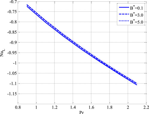
Figure 7. Effect of Prandtl number and coefficient of temperature-dependent term of heat source on local Nusselt number using $M=0.1,Da=7,N=0.1,We=0.1,$$Fs=0.1,\gamma =0.9,A^{*}=0.1,Sc=0.9,$$\epsilon =0.1,{\sigma }_1=0,{\sigma }_2=0,{\sigma }_3=0$.

5.4.2 Effect of Schmidt number ${\mathit{S}}_{\mathit{c}}$ and reaction rate parameter $\mathit{\gamma }$ on the local sherwood number ${\mathit{S}}_{{\mathit{h}}_{\mathit{L}}}$

Figure 8 illustrates the effect of the Schmidt number $S_c$ and the reaction rate parameter $\gamma$ on the local Sherwood number $S_{h_L}$, which represents the mass transfer rate at the surface. The analysis is conducted while keeping the following parameters constant: $M=0.1,Da=7,N=0.1,We=0.1,Fs=0.1,B^{*}=5,A^{*}=0.1,\mathit{Pr}=0.9,\epsilon =0.1,$${\sigma }_1=0,{\sigma }_2=0,{\sigma }_3=0$. The Sherwood number $S_{h_L}$ decreases with increasing distance from the surface. Higher values of $\gamma$ (reaction rate parameter) lead to a more significant reduction in the Sherwood number, meaning mass transfer efficiency decreases with higher reaction rates. The solid line $\gamma =0.1$ represents the case with a low reaction rate. The dashed line $\gamma =0.5$ and dotted line $\gamma =0.9$ show the behavior for increasing $\gamma$. As $\gamma$ increases, the local Sherwood number $S_{h_L}$ declines, indicating a decrease in the mass transfer rate at the boundary. The Schmidt number $S_c$ represents the ratio of momentum diffusivity to mass diffusivity. A higher $S_c$ means lower mass diffusivity, leading to stronger concentration gradients near the surface. The reaction rate parameter $\gamma$ governs the conversion of reactant species into products, reducing the overall concentration of species in the fluid.

Figure 8

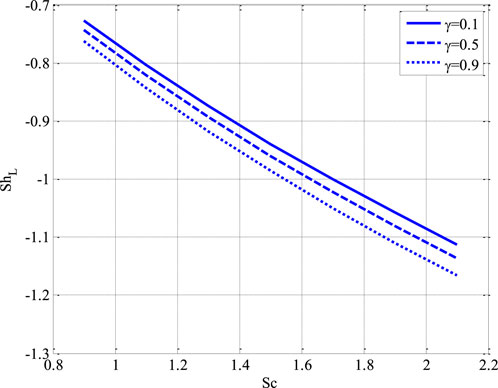
Figure 8. Effect of Schmidt number and reaction rate parameter on local Sherwood number using $M=0.1,Da=7,N=0.1,We=0.1,$$Fs=0.1,B^{*}=5,A^{*}=0.1,\mathit{Pr}=0.9,$$\epsilon =0.1,{\sigma }_1=0,{\sigma }_2=0,{\sigma }_3=0$.

5.4.3 Analyze the effect of oscillatory boundary conditions and contour plots: contour plot for velocity profile

Figure 9 presents a contour plot representing the velocity distribution in a non-Newtonian Williamson fluid flow through a porous medium under various physical effects. The parameters used in the simulation are: $M=0.1,Da=7,N=0.1,We=0.1,Fs=0.1,B^{*}=5,A^{*}=0.1,\mathit{Pr}=0.9,\gamma =0.9,$$Sc=0.9,\epsilon =0.1,{\sigma }_1=0,{\sigma }_2=0,{\sigma }_3=0$. The velocity is highest in the red-coloured region near the bottom-right portion of the figure, indicating a peak flow intensity in this region. As we move away from this region, the velocity gradually decreases, transitioning from red to yellow, green, and finally to blue, representing lower velocity regions. The velocity boundary layer thickness is visible in the transition of colours from the bottom-left (near-wall region) toward the top-right (free-stream region). The velocity boundary layer thickness is visible in the transition of colours from the bottom-left (near-wall region) toward the top-right (free-stream region). The Weissenberg number $W_e=0.1$ represents the fluid’s elastic nature. A low $W_e$ value suggests that the fluid behaves closer to Newtonian behaviour, meaning a more continuous velocity gradient is observed across the flow domain. The magnetic field parameter $M=0.1$ is relatively small, meaning that Lorentz forces are weak, allowing the velocity to develop more freely. The Darcy number $D_a=7$ indicates that the medium has relatively high permeability, enabling a smoother flow through the porous medium. The Prandtl number $P_r=0.9$ suggests that thermal and momentum diffusivity are nearly balanced, meaning that the temperature effects on velocity are moderate. The buoyancy force parameter $N=0.1$ is low, meaning that natural convection effects are not dominant, and the flow remains mostly forced convection driven. The oscillatory boundary condition $ϵ=0.1$ might influence small-scale perturbations in the velocity field, seen as minor irregularities in the contour gradient near the boundary.

Figure 9

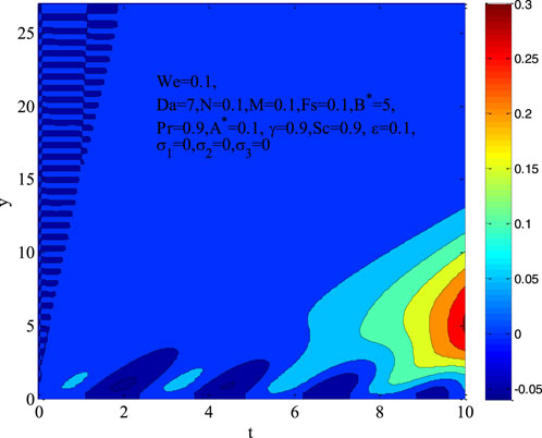
Figure 9. Contour plot for velocity profile using $M=0.1,Da=7,N=0.1,We=0.1,$$Fs=0.1,B^{*}=5,A^{*}=0.1,\mathit{Pr}=0.9,$$\gamma =0.9,Sc=0.9,\epsilon =0.1,{\sigma }_1=0,{\sigma }_2=0,$${\sigma }_3=0$.

5.4.4 Contour plot for temperature profile

Figure 10 presents a contour plot illustrating the temperature distribution in a non-Newtonian Williamson fluid flow through a porous medium under various physical parameters. The simulation is conducted with the following parameter values: $M=0.1,Da=7,N=0.1,We=0.1,Fs=0.1,B^{*}=5,A^{*}=0.1,\mathit{Pr}=0.9,$$\gamma =0.9,Sc=0.9,\epsilon =0.1,{\sigma }_1=0,{\sigma }_2=0,{\sigma }_3=0$. The colour gradient represents temperature intensity, with red and orange regions indicating higher temperatures, while blue and green regions represent lower temperatures. The highest temperature zones (red/orange) are observed near the bottom-right portion of the domain, showing where heat accumulation occurs. As we move away from this region, the temperature gradually decreases, transitioning from red to yellow, green, and blue, illustrating the thermal diffusion process. $B^{*}=5$ signifies a strong internal heat source responsible for elevated temperature levels in certain regions. The Prandtl number $P_r=0.9$ indicates a moderate balance between momentum and thermal diffusivity, leading to a smooth transition of temperature gradients. The oscillatory boundary condition $ϵ=0.1$ may introduce small temperature fluctuations near the bottom edge of the plot, visible as localized variations in temperature contours. A high Darcy number $D_a=7$ implies that the medium has high permeability, allowing better fluid motion and heat conduction. A low Forchheimer number $F_s=0.1$ means that inertial effects are weak, making the temperature distribution uniform without abrupt fluctuations. The buoyancy parameter $N=0.1$ is relatively small, meaning that natural convection does not dominate, and the heat transfer remains primarily conduction-dominated. This temperature distribution is important in thermal engineering applications such as heat exchangers, geothermal energy extraction, polymer processing, and industrial cooling systems.

Figure 10

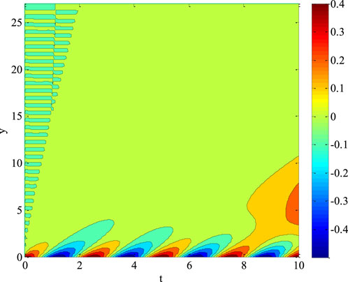
Figure 10. Contour plot for temperature profile using $M=0.1,Da=7,N=0.1,We=0.1,$$Fs=0.1,B^{*}=5,A^{*}=0.1,\mathit{Pr}=0.9,$$\gamma =0.9,Sc=0.9,\epsilon =0.1,{\sigma }_1=0,$${\sigma }_2=0,{\sigma }_3=0$.

5.4.5 Contour plot for concentration profile

Figure 11 presents a contour plot illustrating the concentration distribution in a non-Newtonian Williamson fluid flowing through a porous medium. The concentration field is influenced by various physical parameters, which are set as follows: $M=0.1,Da=7,N=0.1,We=0.1,Fs=0.1,B^{*}=5,A^{*}=0.1,\mathit{Pr}=0.9,\gamma =0.9,$$Sc=0.9,\epsilon =0.1,{\sigma }_1=0,{\sigma }_2=0,{\sigma }_3=0$. The colour gradient represents concentration intensity, with red and orange regions indicating higher concentration levels, while blue and green regions represent lower concentration regions. The highest concentration zones (red/orange) are localized near the bottom-left region of the figure, indicating maximum accumulation of mass transfer near the boundary. The Schmidt number $S_c=0.9$ represents the ratio of momentum diffusivity to mass diffusivity. Since $S_c$ is relatively high, it means that momentum diffuses faster than mass, leading to a thinner concentration boundary layer. The reaction rate parameter $\gamma =0.9$ indicates that chemical reactions consume the solute species, reducing the overall concentration throughout the domain. This explains the gradual decay in concentration levels moving away from the boundary layer. The oscillatory boundary condition $ϵ=0.1$ influences small-scale variations in concentration, which are visible as irregularities in the contour patterns near the bottom of the plot. The buoyancy parameter $N=0.1$ is relatively low, indicating that natural convection effects are weak and mass transport is primarily due to forced convection and diffusion. The Darcy number $D_a=7$ suggests a highly permeable medium, which allows for easier convective mass transfer. This concentration distribution is important in mass transfer engineering applications, such as chemical reaction systems, pollutant dispersion, and pharmaceutical drug delivery.

Figure 11

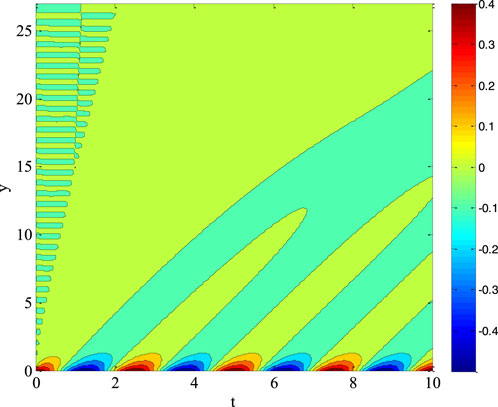
Figure 11. Contour plot for concentration profile using $M=0.1,Da=7,N=0.1,We=0.1,$$Fs=0.1,B^{*}=5,A^{*}=0.1,\mathit{Pr}=0.9,$$\gamma =0.9,Sc=0.9,\epsilon =0.1,{\sigma }_1=0,$${\sigma }_2=0,{\sigma }_3=0$.

5.5 Comparison of proposed and existing schemes

Table 2 presents a comparative analysis of the proposed numerical scheme and the existing second-order Runge-Kutta (RK2) method for solving Stokes’ first problem. For comparison purposes, the corrector stage of the proposed scheme is replaced with the following stage.

${\overline{v}}_i^{n+1}=v_i^n{e}^{1.5\Delta t}+\frac{\left(e^{1.5\Delta t}-1\right)}{1.5}\left[{\left.\frac{\partial v}{\partial t}\right|}_i^n-1.5f_i^n\right](46)$

Table 2

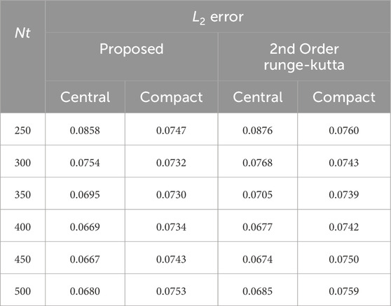
Table 2. Comparison of proposed and existing second-order runge-kutta method for Stokes’ first problem using $Nx\left(gridpoints\right)=50,t_f=1$.

The comparison is performed based on $L_2$ error norms, which measure the numerical accuracy of the computed solutions. $N_x=50$ (Grid Points): A uniform spatial discretization with 50 grid points is used. $t_f=1$: The final time for the simulation is $t=1$. $N_t$ (Time Steps): The comparison is performed for different numbers of time steps ($N_t$ = 250, 300, 350, 400, 450, 500). The proposed numerical scheme achieves a lower $L_2$ errors than the existing second-order Runge-Kutta method, demonstrating its superior accuracy. The error difference is more pronounced at lower-time steps $N_t$ = 250, 300, etc., indicating better stability and precision of the proposed scheme. As $N_t$ increases, the errors in both methods converge, but the proposed scheme maintains a slight accuracy advantage. The compact difference scheme consistently yields lower errors than the central difference scheme in the proposed and existing RK2 methods. The improvement is more noticeable in smaller time steps $N_t$ = 250, 300. This suggests that the compact scheme enhances spatial accuracy, making it more effective for solving Stokes’ first problem. The proposed scheme with compact discretization shows the best performance, achieving the lowest $L_2$ error across all tested $N_t$ values.

These results validate the effectiveness of the two-stage computational method developed in this study, demonstrating its superior numerical performance in solving stochastic Darcy–Forchheimer non-Newtonian flows.

6 Conclusion

This research introduces an innovative computational method for addressing deterministic and stochastic partial differential equations, specifically emphasizing the stochastic Darcy–Forchheimer flow of Williamson fluid over a stationary surface. The suggested two-stage approach integrates a modified time integrator with a second-stage Runge-Kutta algorithm, attaining second-order temporal precision for deterministic models. A sixth-order compact approach is utilized to tackle spatial discretization difficulties, providing great accuracy and processing efficiency. The strategy employs the Euler-Maruyama method to manage Wiener processes in stochastic models, facilitating flexibility to fluctuations in fluid flow dynamics. A numerical scheme has been proposed for solving stochastic time-dependent partial differential equations. The scheme was explicit, and it was comprised of two stages. The compact scheme was chosen to discretize space variable(s). The stability and consistency in the mean square sense of the scheme were presented. The scheme did not require any other scheme to get a solution to the problem. The proposed scheme is implemented in a dimensionless stochastic model of Williamson fluid dynamics, integrating essential physical phenomena such as Darcy–Forchheimer drag and the shear-thinning characteristics of the fluid. Numerical studies on the Stokes first issue indicate that the suggested technique surpasses current second-order Runge-Kutta methods in accuracy, especially in describing the complex relationship between deterministic and stochastic factors affecting the flow. The concluding points can be expressed as.

1. The modification of the proposed scheme performed better than the existing second-order Runge-Kutta method.

2. The compact sixth-order spatial discretization enhances solution accuracy without introducing excessive computational overhead, making it well-suited for high-resolution simulations.

3. Velocity profile declined on average due to the increase in Weissenberg’s number.

4. The velocity profile had dual behaviour on average due to the rising Forchheimer number.

5. The concentration profile declined by raising the reaction rate parameter.

6. The comparative analysis highlights the superior performance of the proposed scheme, offering a reliable alternative to existing methods for solving similar problems.

Finally, a computationally efficient and highly accurate method for non-Newtonian fluids in porous media is introduced, expanding the current state-of-the-art in stochastic fluid dynamics numerical techniques. This paradigm could be further developed in future studies to examine various types of non-Newtonian fluids and more complicated flow configurations, including three-dimensional geometries or transient boundary conditions. Furthermore, there is still room for improvement in the scheme’s optimization for real-time applications and large-scale simulations.

Data availability statement

The original contributions presented in the study are included in the article/supplementary material, further inquiries can be directed to the corresponding author.

Author contributions

MA: Methodology, Software, Supervision, Validation, Visualization, Writing–original draft, Writing–review and editing. KA: Funding acquisition, Investigation, Project administration, Resources, Writing–original draft, Writing–review and editing. YN: Conceptualization, Data curation, Methodology, Validation, Writing–original draft, Writing–review and editing.

Funding

The author(s) declare that financial support was received for the research, authorship, and/or publication of this article.

Acknowledgments

The authors would like to acknowledge the support of Prince Sultan University for paying the Article Processing Charges (APC) of this publication.

Conflict of interest

The authors declare that the research was conducted in the absence of any commercial or financial relationships that could be construed as a potential conflict of interest.

Generative AI statement

The author(s) declare that no Generative AI was used in the creation of this manuscript.

Publisher’s note

All claims expressed in this article are solely those of the authors and do not necessarily represent those of their affiliated organizations, or those of the publisher, the editors and the reviewers. Any product that may be evaluated in this article, or claim that may be made by its manufacturer, is not guaranteed or endorsed by the publisher.

References

1. Cortell R. Similarity solutions for flow and heat transfer of a viscoelastic fluid over a stretching sheet. Int J Nonlinear Mech (1994) 29:155–61. doi:10.1016/0020-7462(94)90034-5

CrossRef Full Text | Google Scholar

2. Mahmoud MAM. The effects of variable fluid properties on MHD Maxwell fluids over a stretching surface in the presence of heat generation/absorption. Chem Eng Comm (2011) 198:131–46. doi:10.1080/00986445.2010.500148

CrossRef Full Text | Google Scholar

3. Pramanik S. Casson fluid flow and heat transfer past an exponentially porous stretching surface in the presence of thermal radiation. Ain Shams Eng J (2014) 5:205–12. doi:10.1016/j.asej.2013.05.003

CrossRef Full Text | Google Scholar

4. Ahmed F, Iqba M. MHD power-law fluid flow and heat transfer analysis through Darcy Brinkman porous media in the annular sector. Int J Mech Sci. (2017) 130:508–17. doi:10.1016/j.ijmecsci.2017.05.042

CrossRef Full Text | Google Scholar

5. Megahed AM. Carreau fluid flow due to nonlinearly stretching sheet with thermal radiation, heat flux, and variable conductivity. Appl Math Mech (2019) 40:1615–24. doi:10.1007/s10483-019-2534-6

CrossRef Full Text | Google Scholar

6. Bilal M, Ashbar S. Flow and heat transfer analysis of Eyring-Powell fluid over stratified sheet with mixed convection. J Egypt Math Soc (2020) 28:40. doi:10.1186/s42787-020-00103-6

CrossRef Full Text | Google Scholar

7. Williamson RV. The flow of pseudoplastic materials. Ind Eng Chem Res. (1929) 21:1108–11. doi:10.1021/ie50239a035

CrossRef Full Text | Google Scholar

8. Nadeem S, Hussain ST, Lee C. Flow of a Williamson fluid over a stretching sheet. Braz J Chem Eng (2013) 30:619–25. doi:10.1590/s0104-66322013000300019

CrossRef Full Text | Google Scholar

9. Khan NA, Khan HA. A boundary layer flows of non-Newtonian Williamson fluid. Nonlinear Eng (2014) 3:107–15. doi:10.1515/nleng-2014-0002

CrossRef Full Text | Google Scholar

10. Malik M, Salahuddin T, Hussain A, Bilal S, Awais M. Homogeneous heterogeneous reactions in Williamson fluid model over a stretching cylinder by using Keller box method. AIP Adv (2015) 5:107227. doi:10.1063/1.4934937

CrossRef Full Text | Google Scholar

11. Khudair WS, Al-Khafajy DGS. Influence of heat transfer on magnetohydrodynamics oscillatory flow for Williamson fluid through a porous medium. Iraqi J Sci (2018) 59:389–97. doi:10.24996/ijs.2018.59.1B.18

CrossRef Full Text | Google Scholar

12. Megahed AM. Steady flow of MHD Williamson fluid due to a continuously moving surface with viscous dissipation and slip velocity. Int J Mod Phys C. (2020) 31:2050019. doi:10.1142/s0129183120500199

CrossRef Full Text | Google Scholar

13. Humane PP, Patil VS, Patil AB. Chemical reaction and thermal radiation effects on magnetohydrodynamics flow of Casson-Williamson nanofluid over a porous stretching surface. Proc Instit Mech Eng E J Process Mech Eng (2021) 235(6):2008–18. doi:10.1177/09544089211025376

CrossRef Full Text | Google Scholar

14. Humane PP, Patil VS, Rajput GR, Shamshuddin M. Dynamics of multiple slip boundaries effect on MHD Casson-Williamson double-diffusive nanofluid flow past an inclined magnetic stretching sheet. Proc Instit Mech Eng Part E J Process Mech Eng (2022) 236(5):1906–26. doi:10.1177/09544089221078153

CrossRef Full Text | Google Scholar

15. Patil VS, Humane PP, Patil AB. MHD Williamson nanofluid flow past a permeable stretching sheet with thermal radiation and chemical reaction. Int J Model Simulat (2023) 43(3):185–99. doi:10.1080/02286203.2022.2062166

CrossRef Full Text | Google Scholar

16. Williamson RV. The flow of pseudoplastic materials. Ind Eng Chem Res (1929) 21(11):1108–11. doi:10.1021/ie50239a035

CrossRef Full Text | Google Scholar

17. Krishnamurthy MR, Prasannakumara BC, Gireesha BJ, Gorla RSR. Effect of chemical reaction on MHD boundary layer flow and melting heat transfer of Williamson nanofluid in porous medium. Eng Sci Technol Int J (2016) 19(1):53–61. doi:10.1016/j.jestch.2015.06.010

CrossRef Full Text | Google Scholar

18. Khan MI, Alzahrani F, Hobiny A, Ali Z. Modeling of Cattaneo-Christov double diffusions (CCDD) in Williamson nanomaterial slip flow subject to porous medium. J Mater Res Technology (2020) 9(3):6172–7. doi:10.1016/j.jmrt.2020.04.019

CrossRef Full Text | Google Scholar

19. Hayat T, Shafiq A, Alsaedi A. Hydromagnetic boundary layer flow of Williamson fluid in the presence of thermal radiation and Ohmic dissipation. Alexandria Eng J (2016) 55(3):2229–40. doi:10.1016/j.aej.2016.06.004

CrossRef Full Text | Google Scholar

20. Nadeem S, Hussain ST, Lee C. Flow of a Williamson fluid over a stretching sheet. Braz J Chem Eng (2013) 30(3):619–25. doi:10.1590/s0104-66322013000300019

CrossRef Full Text | Google Scholar

21. Salahuddin T, Malik MY, Arif H, Bilal S, Awais M. MHD flow of Cattanneo-Christov heat flux model for Williamson fluid over a stretching sheet with variable thickness: using numerical approach. J Magnetism Magn Mater (2016) 401(1):991–7. doi:10.1016/j.jmmm.2015.11.022

CrossRef Full Text | Google Scholar

22. Mohanty D, Mahanta G, Shaw S, Sibanda P. Thermal and irreversibility analysis on Cattaneo–Christov heat flux-based unsteady hybrid nanofluid flow over a spinning sphere with interfacial nanolayer mechanism. J Therm Anal Calorim (2023) 148(21):12269–84. doi:10.1007/s10973-023-12464-y

CrossRef Full Text | Google Scholar

23. Kumar NN, Sastry DRVSRK, Shaw S. Irreversibility analysis of an unsteady micropolar CNT-blood nanofluid flow through a squeezing channel with activation energy-Application in drug delivery. Computer Methods Programs Biomed (2022) 226:107156. doi:10.1016/j.cmpb.2022.107156

PubMed Abstract | CrossRef Full Text | Google Scholar

24. Forchheimer P. H. (1901). Wasserbewegung. Ver. Dtsch. Ing., 45, 1782–1788.

Google Scholar

25. Mukhopadhyay S, De PR, Bhattacharyya K, Layek GC. Forced convective flow and heat transfer over a porous plate in a Darcy-Forchheimer porous medium in presence of radiation. Meccanica (2011) 47(1):153–61. doi:10.1007/s11012-011-9423-3

CrossRef Full Text | Google Scholar

26. Hayat T, Aziz A, Muhammad T, Alsaedi A. Darcy–Forchheimer three-dimensional flow of Williamson nanofluid over a convectively heated nonlinear stretching surface. Commun Theor Phys (2017) 68(3):387–94. doi:10.1088/0253-6102/68/3/387

CrossRef Full Text | Google Scholar

27. Khan MI, Hayat T, Alsaedi A. Numerical analysis for Darcy-Forchheimer flow in presence of homogeneous-heterogeneous reactions. Results Phys (2017) 7:2644–50. doi:10.1016/j.rinp.2017.07.030

CrossRef Full Text | Google Scholar

28. Haider F, Hayat T, Alsaedi A. Flow of hybrid nanofluid through Darcy-Forchheimer porous space with variable characteristics. Alexandria Eng J (2021) 60(3):3047–56. doi:10.1016/j.aej.2021.01.021

CrossRef Full Text | Google Scholar

29. Sadiq MA, Haider F, Hayat T, Alsaedi A. Partial slip in Darcy-Forchheimer carbon nanotubes flow by rotating disk. Int Commun Heat Mass Transfer (2020) 116. doi:10.1016/j.icheatmasstransfer.2020.104641

CrossRef Full Text | Google Scholar

30. Mohanty D, Mahanta G, Shaw S. Analysis of irreversibility for 3-D MHD convective Darcy–Forchheimer Casson hybrid nanofluid flow due to a rotating disk with Cattaneo–Christov heat flux, Joule heating, and nonlinear thermal radiation. Numer Heat Transfer, B: Fundamentals (2023) 84(2):115–42. doi:10.1080/10407790.2023.2189644

CrossRef Full Text | Google Scholar

31. Nayak MK, Shaw S, Ijaz Khan M, Pandey VS, Nazeer M. Flow and thermal analysis on Darcy-Forchheimer flow of copper-water nanofluid due to a rotating disk: a static and dynamic approach. J Mater Res Technology (2020) 9(4):7387–408. doi:10.1016/j.jmrt.2020.04.074

CrossRef Full Text | Google Scholar

32. Mohanty D, Mahanta G, Chamkha AJ, Shaw S. Numerical analysis of interfacial nanolayer thickness on Darcy-Forchheimer Casson hybrid nanofluid flow over a moving needle with Cattaneo-Christov dual flux. Numer Heat Transfer, A: Appl (2023) 1–25. doi:10.1080/10407782.2023.2263906

CrossRef Full Text | Google Scholar

33. Umavathi JC, Ojjela O, Vajravelu K. Numerical analysis of natural convective flow and heat transfer of nanofluids in a vertical rectangular duct using Darcy-Forchheimer-Brinkman model. Int J Therm Sci (2017) 111:511–24. doi:10.1016/j.ijthermalsci.2016.10.002

CrossRef Full Text | Google Scholar

34. Nadeem S, Ishtiaq B, Alzabut J, Ghazwani HA. Entropy generation for exact irreversibility analysis in the MHD channel flow of Williamson fluid with combined convective-radiative boundary conditions. Heliyon (2024) 10(4):e26432. doi:10.1016/j.heliyon.2024.e26432

PubMed Abstract | CrossRef Full Text | Google Scholar

35. Marchioro C, Pulvirenti M. Vortex methods in two-dimensional fluid mechanics. In: Lecture notes in physics. Berlin, Germany: Springer (1984).

Google Scholar

36. Vishik MI, Komechi AI, Fursikov AI. Some mathematical problems of statistical hydrodynamics. Russ Math Surv (1979) 34:149–234. doi:10.1070/rm1979v034n05abeh003906

CrossRef Full Text | Google Scholar

37. Gawedzki K. Soluble models of turbulent transport. In: S Nazarenko, and O Zaboronski, editors. Non-equilibrium statistical mechanics and turbulence. Cambridge, UK: Cambridge Uniersity Press (2008). p. 47–107.

Google Scholar

38. Khan AA, Zafar S, Khan A, Abdeljawad T. Tangent hyperbolic nanofluid flow through a vertical cone: unraveling thermal conductivity and Darcy–Forchheimer effects. Mod Phys Lett B (2024) 39:2450398. doi:10.1142/s0217984924503986

CrossRef Full Text | Google Scholar

39. Fatima N, Kousar N, Ur Rehman K, Shatanawi W. Computational analysis of heat and mass transfer in magnetized Darcy-forchheimer hybrid nanofluid flow with porous medium and slip effects. CMES-Computer Model Eng and Sci (2023) 137(3):2311–30. doi:10.32604/cmes.2023.026994

CrossRef Full Text | Google Scholar

40. Bensoussan A, Teman R. Équations stochastiques du type Navier–Stokes. J Funct Anal (1973) 13:195–222. doi:10.1016/0022-1236(73)90045-1

CrossRef Full Text | Google Scholar

41. Pope SB. On the relationship between stochastic Lagrangian models of turbulence and second-moment closures. Phys Fluids (1994) 6:973–85. doi:10.1063/1.868329

CrossRef Full Text | Google Scholar

42. Holm DD. Variational principles for stochastic fluid dynamics. Proc R Soc A (2015) 471:20140963. doi:10.1098/rspa.2014.0963

PubMed Abstract | CrossRef Full Text | Google Scholar

43. Bharathi V, Prakash J. Zeta potential and activation energy effects in an EMHD non-Newtonian nanofluid flow over a wedge with Darcy-Forchheimer porous medium. Numer Heat Transfer, Part A: Appl (2024) 1–28. doi:10.1080/10407782.2024.2316212

CrossRef Full Text | Google Scholar

44. Prakash J, Tripathi D, Bég OA. Computation of EMHD ternary hybrid non-Newtonian nanofluid over a wedge embedded in a Darcy-Forchheimer porous medium with zeta potential and wall suction/injection effects. Int J Ambient Energ (2023) 44(1):2155–69. doi:10.1080/01430750.2023.2224339

CrossRef Full Text | Google Scholar

45. Lund LA, Fadhel MA, Prakash J, Dhange M, Verma A, Ramesh K. Duality and stability analysis of radiatively magnetized rotating CNTs/C₂ H₆ O₂ + H₂ O nanofluid flow over a stretching/shrinking surface. Int J Appl Comput Mathematics (2024) 10(1):25. doi:10.1007/s40819-023-01661-w

CrossRef Full Text | Google Scholar

46. Ahmed OS, Eldabe NT, Abou-zeid MY, El-kalaawy OH, Moawad SM. Numerical treatment and global error estimation for thermal electro-osmosis effect on non-Newtonian nanofluid flow with time periodic variations. Scientific Rep (2023) 13:14788. doi:10.1038/s41598-023-41579-3

PubMed Abstract | CrossRef Full Text | Google Scholar

Glossary

${\mathbf{u}}^{\mathbf{*}},{\mathbf{v}}^{\mathbf{*}}$ Horizontal and vertical components of velocity $\left(m.s^{-1}\right)$

${\mathbf{x}}^{\mathbf{*}},{\mathbf{y}}^{\mathbf{*}}$ Cartesian coordinates $\left(m\right)$

$\mathbf{T}$ Temperature of the fluid $\left(K\right)$

${\mathbf{T}}_{\mathbf{w}}$ Wall Temperature $\left(K\right)$

${\mathbf{T}}_{\mathbf{\infty }}$ Free Stream temperature (K)

$\mathbf{\alpha }$ Thermal Diffusivity $\left(m^2.s^{-1}\right)$

${\mathbf{k}}_{\mathbf{p}}$ Permeability of porous medium $\left(m^2\right)$

$\mathbf{\nu }$ Kinematic viscosity $\left(m^2.s^{-1}\right)$

$\mathbf{g}$ Gravity $\left(m.s^{-2}\right)$

$\mathbf{\Gamma }$ material fluid parameter $\left(s\right)$

${\mathbf{c}}_{\mathbf{p}}$ Specific heat capacity $\left(J{kg}^{-1}K\right)$

$\mathbf{N}$ Buoyancy ratio

$\mathbf{M}$ Magnetic parameter

${\mathbf{W}}_{\mathbf{e}}$ Weissenberg number

$\mathbf{\epsilon }$ dimensionless parameter

$\mathbf{\gamma }$ reaction rate parameter

$\mathbf{C}$ Concentration $\left(mol.m^{-3}\right)$

${\mathbf{C}}_{\mathbf{\infty }}$ Free stream concentration $\left(mol.m^{-3}\right)$

${\mathbf{C}}_{\mathbf{w}}$ local couple stress coefficient at the wall $\left(mol.m^{-3}\right)$

$\mathbf{\rho }$ Density of fluid $\left(kg.m^{-3}\right)$

$\mathbf{\sigma }$ Electrical Conductivity $\left(S.m^{-1}\right)$

${\mathbf{B}}_{\mathbf{0}}$ Magnetic field vector $\left(A/m\right)$

$\mathbf{D}$ Mass Diffusivity $\left(m^2.s^{-1}\right)$

${\mathbf{\beta }}_{\mathbf{T}}$ coefficient of thermal expansion of the fluid $\left(K^{-1}\right)$

${\mathbf{\beta }}_{\mathbf{C}}$ coefficient of solutal expansion of the fluid $\left(K^{-1}\right)$

${\mathbf{k}}_{\mathbf{c}}$ Reaction rate parameter $\left(s^{-1}\right)$

$\overline{\mathbf{b}}$ Forchheimer coefficient $\left(m^{-1}\right)$

${\mathbf{D}}_{\mathbf{a}}$ Darcy’s number

${\mathbf{P}}_{\mathbf{r}}$ Prandtl number

${\mathbf{S}}_{\mathbf{c}}$ Schmidt number

${\mathbf{F}}_{\mathbf{S}}$ Forchheimer number