Frequency domain estimation method of the characteristic period of the P wave of earthquakes

Early warning system earthquake alerts exploit the time delay that the surface waves have in reference to the P waves and estimate the magnitude based on the interpretation of the specific parameters of the P waves. One of the most commonly used parameters for estimating the moment magnitude of an earthquake is the characteristic period measured in the first 3 s after the appearance of the P wave. The classic method determines the characteristic period in the time domain by using the velocity and displacement waves of the acquired samples. In this paper, we present a new method for estimating the characteristic period through its corresponding frequency. This method includes zero padding of the P-wave sequence, conversion of the extended sequence from the time domain to the frequency domain, identification of local frequency maxima, and calculation of the weighted average of the frequency based on the identified maxima. Tests conducted on synthetic signals, as well as standard deviation evaluation tests for simultaneous recordings at several seismic stations, revealed better performance than the classic method in terms of noise immunity and number of false alarms.

1 Introduction

The intense ground motions caused by an earthquake pose a major hazard to the population living near the epicenter and can cause substantial damage to roads, buildings, and other infrastructure. Among natural disasters, earthquakes account for approximately one-fifth of economic losses and are responsible for approximately 20,000 deaths per year. A destructive earthquake cannot be predicted accurately at the moment or place of its occurrence. However, earthquake early warning systems (EEWS) can provide an estimation of the approaching event. EEWS can trigger anticipative alarms because the onset of an earthquake is achieved by non-destructive primary P waves and continues with destructive surface waves. P waves have a higher travel speed; they will reach the destination first and can be a source of information regarding the destructive waves that will reach the destination later. Moreover, P-wave-based EEWS can work in tandem with seismicity indicator-based systems that make use of the Gutenberg–Richter law to increase the probability of detection of major earthquakes [1–3].

After several decades of development, EEWS are currently operational and provide alerts to populations (Japan [4, 5], Taiwan [6, 7], Mexico [8], and South Korea [9]), institutions, or limited users (India [10], Romania [11], Turkey [12], and the West Coast of the United States [13]), or are under development or testing (Italy [14], Chile, Costa Rica, EI Salvador, Nicaragua, Switzerland, Israel, Beijing, and the Fujian region of China) [15].

The main component of an EEW system is the algorithm that estimates the magnitude of an earthquake. The assessment is performed using the velocity and displacement waveforms and must contain as much of the low-frequency component of the frequency spectrum as possible to avoid magnitude saturation [16].

Among the first P-wave parameters used for magnitude estimation is the predominant period, defined as the period corresponding to the maximum amplitude in the frequency spectrum of displacement [17, 18]. An approach to the predominant period based on the velocity wave known as the τp method is presented in [19]. Because this method contains numerous limitations related to the sampling frequency and signal processing, an improved version was proposed in [20], where the predominant period is continuously calculated, and its maximum value (τp max) can be determined. Another magnitude estimation parameter is the characteristic period τc. This refers to both velocity and displacement waves, which are much more stable than τp max [21]. In current studies, the characteristic period is the most commonly used parameter for magnitude estimation with regard to the peak of the displacement wave (Pd) [22, 23] or alongside other geophysical parameters as input data for neural networks [24, 25].

However, the characteristic period of a specific earthquake, computed from different recording stations, exhibits large dispersion in terms of standard deviation due to local conditions, noise, and artifacts and thus may trigger false alarms or mute real ones. In order to evaluate the characteristic period of the P wave, we propose a new method based on the accurate determination of local maxima within the displacement wave’s frequency spectrum. Its performance is evaluated using both synthesized and recorded waveforms, yielding better results than the standard approaches.

2 Methods

To define the characteristic period [21], the vertical components of the ground displacement wave u(t) and velocity $\dot{u}$ (t) were used, with the ratio r being

$\mathit{r}=\frac{{\int }_{\mathbf{0}}^{{\mathit{t}}_{\mathbf{0}}}{\dot{\mathit{u}}}^{\mathbf{2}}\left(\mathit{t}\right)\mathit{d}\mathit{t}}{{\int }_{\mathbf{0}}^{{\mathit{t}}_{\mathbf{0}}}{\mathit{u}}^{\mathbf{2}}\left(\mathit{t}\right)\mathit{d}\mathit{t}},(1)$

where the integration is over the time interval (0, t₀) after the onset of the P wave. In most of the existing EEWS, t₀ is set to 3 s, and any straightforward implementation of Equation 1 belongs to the time domain methods used to evaluate the characteristic period. They have been adopted by the scientific community as a benchmark and as a standard specification in most of the existing EEWS [22, 26]. Using Parseval’s theorem, according to which the energy of an aperiodic signal or the power of a periodic signal in the time domain is equal to the energy or power in the frequency domain, the results of Equation 2 are obtained and further exploited to develop frequency-domain methods.

$\mathit{r}=\frac{\mathbf{4}{\mathit{\pi }}^{\mathbf{2}}{\int }_{\mathbf{0}}^{\mathit{\infty }}{\mathit{f}}^{\mathbf{2}}{\left|\widehat{\mathit{u}}\left(\mathit{f}\right)\right|}^{\mathbf{2}}\mathit{d}\mathit{f}}{{\int }_{\mathbf{0}}^{\mathit{\infty }}{\left|\widehat{\mathit{u}}\left(\mathit{f}\right)\right|}^{\mathbf{2}}\mathit{d}\mathit{f}}=\mathbf{4}{\mathit{\pi }}^{\mathbf{2}}〈{\mathit{f}}^{\mathbf{2}}〉,(2)$

where f is the frequency, û(f) is the frequency spectrum of the displacement wave u(t), and $〈f^2〉$ is the average of f² weighted by |û(f)|², hereafter denoted by f_C.²

The characteristic period is defined according to Equation 3:

${\mathit{\tau }}_{\mathit{c}}=\frac{\mathbf{1}}{\sqrt{{\mathit{f}}_{\mathit{c}}^{\mathbf{2}}}}=\frac{\mathbf{2}\mathit{\pi }}{\sqrt{\mathit{r}}}.(3)$

Although the characteristic period of the P wave is calculated based on the ratio r, as can be seen in Equation 3, the characteristic period can also be expressed based on the frequency spectrum of the displacement. More precisely, the squared characteristic frequency is the average of the squared frequencies weighted by the square of the amplitudes in the frequency spectrum.

${\mathit{f}}_{\mathit{c}}^{\mathbf{2}}=\frac{{\mathit{A}}_{\mathbf{1}}^{\mathbf{2}}·{\mathit{f}}_{\mathbf{1}}^{\mathbf{2}}+{\mathit{A}}_{\mathbf{2}}^{\mathbf{2}}·{\mathit{f}}_{\mathbf{2}}^{\mathbf{2}}+···+{\mathit{A}}_{\mathit{n}}^{\mathbf{2}}·{\mathit{f}}_{\mathit{n}}^{\mathbf{2}}}{{\mathit{A}}_{\mathbf{1}}^{\mathbf{2}}+{\mathit{A}}_{\mathbf{2}}^{\mathbf{2}}+···+{\mathit{A}}_{\mathit{n}}^{\mathbf{2}}},(4)$

where A₁ … A_n are the amplitudes of the spectral components, and f₁….f_n are the frequencies of the spectral components. These values of the spectral components are obtained by applying a fast Fourier transform (FFT) to the displacement sequence in the time domain. There are many reported results in using FFT to differentiate seismic signals from ambient signals or those produced by explosions because the generated spectra can be distinguished [27, 28], but to date, no straightforward implementation of Equation 4 in EEWS makes use of the τc parameter.

Furthermore, the proposed development implies a better localization of the local maxima points in the discrete-time Fourier transform (DTFT)-associated function and thus minimizes the picket fence effect [29].

Three methods for increasing frequency resolution were considered: zero padding [30], FFT interpolation [31], and windowing [32]. Due to the specific nature of the seismic signals, a short analysis qualifies the zero-padding technique as the best candidate because:

- interpolation techniques are inefficient when the analyzed signal is a multi-frequency one, with massive overlap of adjacent energy bands;

- except for a rectangular window that is similar in the frequency domain with zero padding, the remaining windowing techniques reduce the signal’s amplitude toward the edges, and thus, the first points in the earthquake spectrum (the ones with the most important information) are affected;

- there are no computational or timing constraints that could impact the practical deployment of the zero-padding technique because the FFT algorithm is highly efficient, and the time required to calculate frequency spectrum, even with sequences of zeros ten times larger than signal length, is of the order of milliseconds.

For the presented method, zero padding is the solution used to reduce the distance between bins in frequency by increasing the sequence of the investigated signal by adding zeros to its end before the FFT is applied. The extension of the seismic signal with null samples will not negatively influence the application of the method because it is only desired to obtain a specific length of the signal. Studies prove that this is a viable alternative method that improves the readability of the signal frequency [33, 34]. The increased length of the signal has the consequence of decreasing the width between consecutive spectral lines, resulting in a finer frequency resolution.

After applying zero padding, the local maxima in the frequency spectrum are identified, and the characteristic frequency is evaluated as

${\mathit{f}}_{\mathit{c}}^{\mathbf{2}}=\frac{{\mathit{A}}_{\mathbf{1}}^{\mathbf{2}}·{\mathit{f}}_{\mathbf{1}}^{\mathbf{2}}+{\mathit{A}}_{\mathbf{2}}^{\mathbf{2}}·{\mathit{f}}_{\mathbf{2}}^{\mathbf{2}}+\dots +{\mathit{A}}_{\mathit{k}}^{\mathbf{2}}·{\mathit{f}}_{\mathit{k}}^{\mathbf{2}}}{{\mathit{A}}_{\mathbf{1}}^{\mathbf{2}}+{\mathit{A}}_{\mathbf{2}}^{\mathbf{2}}+\dots +{\mathit{A}}_{\mathit{k}}^{\mathbf{2}}},(5)$

where k, A_k, and f_k are the number of identified maxima, the amplitude, and the frequency, respectively.

Structurally, as can be seen in Figure 1, the method of calculating the characteristic period in the frequency spectrum includes the following steps: from the earthquake displacement waveform (a), the first 3 s of the signal are extracted (b), the retrieved sequence is padded with zeros (c), and FFT is applied to obtain the frequency spectrum (d). At the level of the frequency spectrum, the local maxima (e) are identified, through which the weighted average of the characteristic frequency is calculated (Equation 5), and implicitly, its inverse is also calculated.

Figure 1

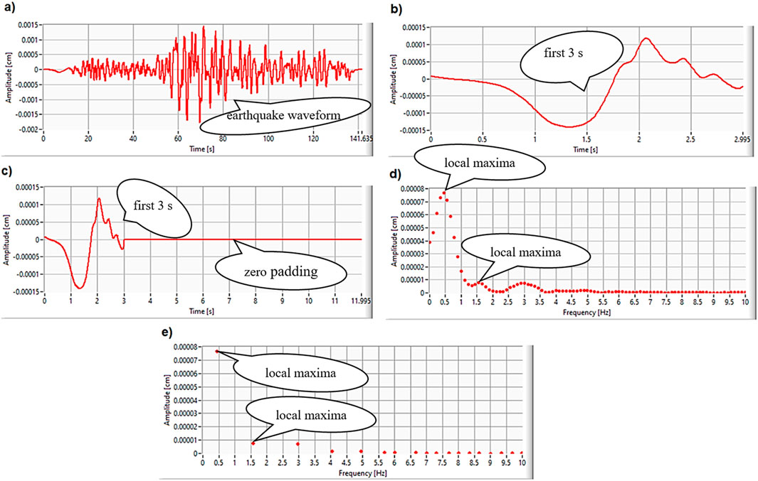
Figure 1. Attainment of the characteristic period of the seismic P-wave estimation in the frequency domain: (A) Display a recorded seismic waveform; (B) Extract the first 3 s of the signal; (C) Pad the sequence with zeros; (D) Apply FFT; (E) Identify the local maxima.

To test the proposed method, a comparative study was carried out between the classic method, from the time domain that uses the ratio between speed and displacement (M1), the method from the frequency domain based on Equation 4 to calculate the characteristic frequency (M2), and the proposed method (M3) based on Equation 5. The test signals used to calculate the characteristic frequency and characteristic period were synthesized by summing sinusoidal signals with imposed frequencies and amplitudes. The reference frequency against which the absolute error was calculated was obtained using the signal synthesis values (the amplitudes and frequencies of the sinusoidal signals were summed to obtain the test signals). The framework of signal acquisition is similar to the physical one used in the acquisition of seismic signals: sampling frequency, 200 Hz; acquisition time, 3 s; total number of acquired points, 600.

3 Results

A method for calculating the characteristic period of the P wave of earthquakes based on the frequency spectrum of the displacement wave was developed. Three types of validation tests were carried out: one with signals containing a single spectral component (a pure sinusoidal signal), one with signals with two spectral components, and one with three spectral components with different frequency and amplitude values.

3.1 Testing using a signal with a single spectral component

A set of sinusoidal signals of 3 units amplitude was used, for which the frequency was varied between 0.3 Hz and 20 Hz, the range covering the area of interest for EEW systems (Figure 2). The variation step is 0.1 Hz. For each signal, the characteristic frequency and the characteristic period were calculated by three methods (time-domain classic method M1, frequency-domain method M2, and proposed method M3), and the absolute errors compared to the reference were determined. The column of graphs on the left in Figure 2 shows the absolute errors for the characteristic frequency, and the column on the right shows the results for the characteristic period for the three methods M1, M2, and M3.

Figure 2

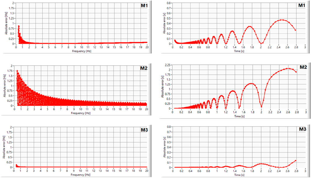
Figure 2. Absolute error graph of the three compared methods, in frequency-domain (left) and time-domain (right) calculations, for a singular spectrum signal.

It can be observed that for all methods, the errors increase with a decrease in the frequency and implicitly with an increase in the period. The M2 method presents almost twice as many absolute errors as the classical method M1, whereas the proposed method M3 presents errors reduced to at least one-third of the number presented by the classical method.

3.2 Testing using a signal having two spectral components

A set of synthetic signals from a sinusoidal signal of 8 units amplitude and 0.9 Hz frequency was used, as was a sinusoidal signal of 3 units amplitude, for which the frequency was varied between 0.3 and 20 Hz (Figure 3). For each signal, the characteristic frequency and the characteristic period were determined by the three methods, and the absolute errors were then compared to the reference (parameters imposed on the signal synthesis) and plotted in Figure 3. Within this test for all methods, the errors increase with decreasing frequency and increasing period. The M2 method presents almost twice as many errors as the classical method M1, whereas the errors of the proposed method M3 were reduced to at least one-third of the number presented by the classical method.

Figure 3

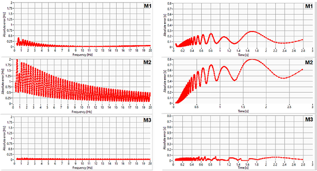
Figure 3. Absolute error graph of the three compared methods, in frequency-domain (left) and time-domain (right) calculations, for a multicomponent signal with two spectra.

3.3 Testing using a signal having three spectral components

A set of synthetic signals from a sinusoidal signal of 8 units amplitude and 0.9 Hz frequency, a sinusoidal signal of 2.7 units amplitude and 1.3 Hz frequency, and a sinusoidal signal of 3 units amplitude, for which the frequency was varied between 0.3 and 20 Hz, was used (Figure 4). Similarly, the frequencies and characteristic periods were calculated using the three methods. Comparing the absolute errors from Figures 3, 4 in the corresponding domain, it is found that there is no change in the ratio between the errors of the three methods with an increase in the number of harmonics. This asserts that the proposed method leads to a reduced standard deviation compared to the classical method, as well as for multicomponent waveforms.

Figure 4

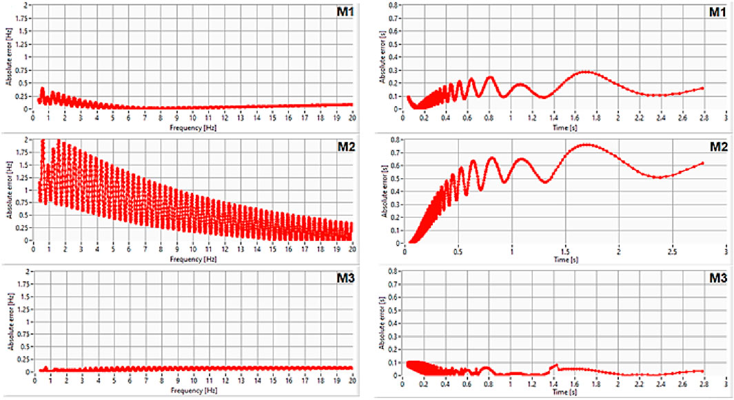
Figure 4. Absolute error graph of the three compared methods, in frequency-domain (left) and time-domain (right) calculations, for a multicomponent signal with three spectra.

3.4 Performance under noisy conditions

In seismic monitoring, accurate data are essential for understanding the behavior of structures under stress or seismic activity. Noise can interfere with measurements, leading to false readings or missed events. A high signal-to-noise ratio (SNR) ensures that seismic signals and vibrations are captured clearly, providing reliable data for analysis.

• An SNR below 10 dB indicates poor signal quality, requiring significant noise reduction.

• An SNR between 10 dB and 20 dB is useable but may need some filtering.

• An SNR above 20 dB ensures reliable data with minimal noise interference.

A sinusoidal signal of 3V amplitude was used for the comparative evaluation of methods M1 and M3 in the presence of noise, over which an additional white noise of 1V amplitude was added, as represented in Figure 5. For this case, the signal/noise ratio is 9.5 dB.

Figure 5

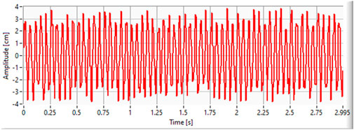
Figure 5. Sinusoidal signal summed with white noise.

FFT performs averaging operations in calculation by its nature. Moreover, the proposed method M3 uses only the distinct peaks obtained after zero padding. Considering the fact that the time-domain energy of the noise is distributed in frequency over the entire spectrum, M3 obtains superior results to the M1 method in the presence of high noise. The results of applying FFT on the signal with noise after zero padding are represented in Figure 6.

Figure 6

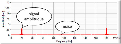
Figure 6. Applying FFT to a signal with noise after zero padding.

Figure 7 presents a comparative analysis of the absolute error in determining the τ_c parameter for a sinusoidal signal frequency variation of up to 20 Hz.

Figure 7

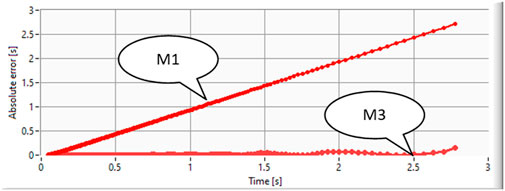
Figure 7. Absolute error comparison for M1 and M3 applied on a signal with a frequency up to 20 Hz.

3.5 Standard deviation evaluation

A comparison was made between the classical method and the proposed method, subjected to the dispersion of the values of the characteristic period of an earthquake when several stations that simultaneously record an event are considered. Thus, the average value of the characteristic period and the standard deviation were calculated for a given earthquake characterized by the seismic waves recorded at N different stations. This reasoning was applied to the vertical waves of ten earthquakes that occurred in 2021, 2022, and 2023, with the main parameters listed in Table 1, whose records at 200 Hz were taken from the ESM Database [35].

Table 1

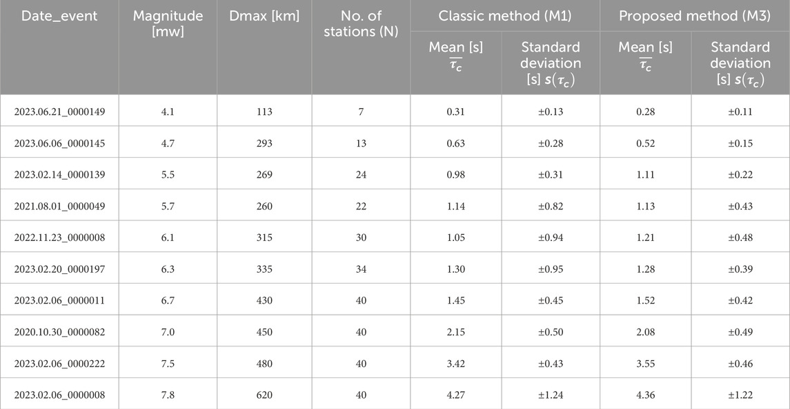
Table 1. Standard deviation of the seismic characteristic period calculated with the time-domain method (M1) and the proposed method (M3).

D_max represents the distance between the epicenter and the farthest station from which the recording of the considered earthquake was used. N is the number of stations from which records of a certain earthquake were taken. The average characteristic period was calculated as shown in Equation 6:

$\overline{{\mathit{\tau }}_{\mathit{c}}}=\frac{{\sum }_{\mathbf{1}}^{\mathit{N}}{{\mathit{\tau }}_{\mathit{c}}}_{\mathit{i}}}{\mathit{N}}.(6)$

The standard deviation was determined using Equation 7:

$\mathit{s}\left({\mathit{\tau }}_{\mathit{c}}\right)=\frac{{\sum }_{\mathbf{1}}^{\mathit{N}}{\left(\overline{{\mathit{\tau }}_{\mathit{c}}}-{{\mathit{\tau }}_{\mathit{c}}}_{\mathit{i}}\right)}^{\mathbf{2}}}{\mathit{N}-\mathbf{1}}.(7)$

The results in Table 1 show that using the proposed method (M3) leads to a smaller dispersion for each earthquake than the classic method (M1).

Accuracy of EEWS alerts. It is not yet possible to absolutely and rapidly determine the final effects of an earthquake rupture based on the data recorded at the beginning of the earthquake. Hence, EEWS seldom provide false alarms or miss alerts [36]. A false alarm arises when parameter estimation exceeds the alert threshold, although the ground movement after the completed rupture does not reach the evaluated effect. Similarly, a missed alert arises when parameter estimation does not reach the alert threshold, although the ground movement after the completed rupture exceeds the evaluated effect [37]. Even if it is considered that EEWS can perfectly determine the average value of ground motion, the accuracy of EEWS is determined by the variation from the average value of the ground motion metrics that the EEW system uses to evaluate ground motion [38]. Under these conditions, if two methods for evaluating ground motion metrics are considered to have the same mean value for an earthquake but different standard deviations s₁ and s₂, as shown in Figure 8, the number of false alarms, given by the area of the shaded surface, is higher for the higher standard deviation. It results in one of the major advantages of using the proposed method (M3) instead of the classic one (M1).

Figure 8

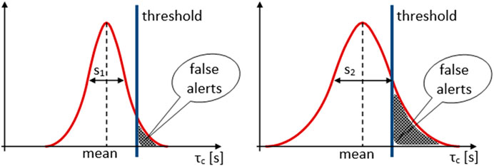
Figure 8. Cause–effect relationship between EEW false alarms, threshold values, and standard deviations.

4 Discussion

The proposed method was tested to determine the characteristic period by calculating the characteristic frequency from the frequency spectrum of the signal. Testing was carried out in two ways: by simulation and by calculation of real P-wave signals obtained from earthquake recordings.

4.1 Testing the method by simulation

Synthesized signals with precisely known frequency/periods were used for testing. For these signals, the frequency/period was calculated using the classical method M1 from the time domain, which uses the ratio between speed and displacement; the method M2 based on Equation 4, which is derived directly from the classical method by correspondence in frequency; and the proposed method, M3.

Method M1 provides results in terms of time, and M2 and M3 provide results in terms of frequency. To make comparisons from the point of view of absolute errors both as characteristic period and characteristic frequency, the characteristic period obtained by M1 was converted into characteristic frequency, and the characteristic frequencies obtained by M2 and M3 were converted into characteristic periods.

Tests were carried out with pure sinusoidal signals and with sinusoidal signals with harmonics, and graphs of the absolute errors obtained for the three methods were plotted. The following observations were made:

• Switching to the frequency domain (M2) did not provide better results than the classical method.

• The application of the M3 method leads to a reduction in the relative errors for all test variants with synthesized signals, regardless of the number or frequency values of the harmonics.

• Because P-wave sequences are limited to 3 s, signals with frequencies below 0.3 Hz or periods of more than 3 s will contain less than one period of the useful signal.

Thus, for all methods, the errors increase at low frequencies and implicitly at long periods and represent the area where saturation occurs for large earthquakes.

4.2 Testing the method with real P waves

Because this work refers to a method of estimating the characteristic period of the P wave of earthquakes, testing with real P waves was carried out only for the purpose of estimating the period and validating the simulation testing. Forecasting the magnitude based on the P wave is dependent on the soil structure in the direction of earthquake propagation from the epicenter to the seismic station where the wave is recorded, which is geophysically dependent. For the test, 290 seismic recordings from 10 different earthquakes recorded at different stations were used. For each recording, the characteristic period was determined using M1 and M3. The periods were grouped by the ten earthquake events, and the average value and standard deviation were calculated for each event. As shown in Table 1, the standard deviation calculated for the proposed method has lower values than the classical method of up to 6.3 Mw, corresponding to a characteristic period of 1.30 s, with no other specific conditions where the performance differs. For earthquakes above this value, no improvements were observed compared to the classical method.

EEW systems use a threshold for both the characteristic period and maximum amplitude. For the characteristic period, the threshold was set to 1 s. The alarm is sent if the threshold imposed for the characteristic period is exceeded, along with the threshold for the maximum amplitude. Given that the EEW alarm is triggered for a threshold of 1 s corresponding to 5.5–5.7 Mw, which is the interval in which the proposed method provides a better standard deviation, we consider that this method can be used to increase the EEW performance.

5 Conclusion

Most earthquake early warning systems are used to predict the event magnitude and the peak ground acceleration parameters attained from the initial P waves recorded at close seismic stations. Commonly, the peak amplitudes of displacement, along with the characteristic period and integral of the squared velocity, are used in specific algorithms to compute the level of danger and the necessity for EEWS to trigger an emergency alarm. Estimating the characteristic period τc involves inputs such as velocity and acceleration from multiple P waves that are similarly recorded at several seismic stations. As τc increases with the magnitude of an earthquake and is independent of the distance between the earthquake epicenter and an observation station up to a few hundred kilometers away, it is a key factor in EWS regional seismic prediction.

The proposed method for calculating the characteristic period of the seismic P wave in the frequency domain has a lower standard deviation than the classical method. Tests carried out using synthetic signals, with a single tone or with harmonic content, reveal that the determination errors of the characteristic period are smaller when using this method. Statistical tests to evaluate the standard deviation, in which earthquake records from several stations were interpreted, also revealed the superior behavior of the proposed method up to 6.3 Mw, with direct consequences in reducing the number of false alarms. Thus, it is suited for EEWS systems that use the τc parameter in alarm decision algorithms. In this context, we consider that this method can be used with good results in magnitude prediction applications based on the characteristic period of the initial wave.

Data availability statement

The raw data supporting the conclusions of this article will be made available by the authors, without undue reservation.

Author contributions

CD: writing–original draft. ES: writing–review and editing. MT: writing–original draft.

Funding

The author(s) declare that financial support was received for the research, authorship, and/or publication of this article. This research was funded by the European Regional Development Fund, grant number 7227/19.11.2021 (SMIS code 137414) — “Seismic warning system with automatic unlocking of entrance doors with interphone.” The article publishing charge was funded by “Gheorghe Asachi” Technical University of Iași, România.

Conflict of interest

The authors declare that the research was conducted in the absence of any commercial or financial relationships that could be construed as a potential conflict of interest.

Publisher’s note

All claims expressed in this article are solely those of the authors and do not necessarily represent those of their affiliated organizations, or those of the publisher, the editors and the reviewers. Any product that may be evaluated in this article, or claim that may be made by its manufacturer, is not guaranteed or endorsed by the publisher.

References

1. Iwata D, Nanjo KZ. Adaptive estimation of the Gutenberg–Richter b value using a state space model and particle filtering. Scientific Rep (2024) 14(1):4630. doi:10.1038/s41598-024-54576-x

PubMed Abstract | CrossRef Full Text | Google Scholar

2. Taroni M, Vocalelli G, De Polis A. Gutenberg–Richter B-value time series forecasting: a weighted likelihood approach. Forecasting (2021) 3(3):561–9. doi:10.3390/forecast3030035

CrossRef Full Text | Google Scholar

3. Rafiei MH, Adeli H. NEEWS: a novel earthquake early warning model using neural dynamic classification and neural dynamic optimization. Soil Dyn Earthquake Eng (2017) 100:417–27. doi:10.1016/j.soildyn.2017.05.013

CrossRef Full Text | Google Scholar

4. Kodera Y, Hayashimoto N, Tamaribuchi K, Noguchi K, Moriwaki K, Takahashi R, et al. Developments of the nationwide earthquake early warning system in Japan after the 2011 M w 9.0 Tohoku-Oki earthquake. Front Earth Sci (2021) 9. doi:10.3389/feart.2021.726045

CrossRef Full Text | Google Scholar

5. Goltz JD, Evelyn R. Imminent warning communication: earthquake early warning and short-term forecasting in Japan and the US. In: Disaster risk communication: a challenge from a social psychological perspective (2020). p. 121–53.

Google Scholar

6. Wu Y-M, Mittal H, Chen D-Y, Hsu T-Y, Lin P-Y. Earthquake early warning systems in Taiwan: current status. J Geol Soc India (2021) 97:1525–32. doi:10.1007/s12594-021-1909-6

CrossRef Full Text | Google Scholar

7. Kumar R, Mittal H, Sharma B. Earthquake genesis and earthquake early warning systems: challenges and a way forward. Surv Geophys (2022) 43(4):1143–68. doi:10.1007/s10712-022-09710-7

CrossRef Full Text | Google Scholar

8. Cuéllar A, Espinosa-Aranda JM, Suárez R, Ibarrola G, Uribe A, Rodríguez FH, et al. The Mexican Seismic Alert System (SASMEX): its alert signals, broadcast results and performance during the M 7.4 Punta Maldonado earthquake of March 20th. In: Early warning for geological disasters: scientific methods and current practice (2012). p. 71–87.

Google Scholar

9. Sheen D-H, Park J-H, Chi H-C, Hwang E-H, Lim I-S, Jeong Seong Y, et al. The first stage of an earthquake early warning system in South Korea. Seismological Res Lett (2017) 88(6):1491–8. doi:10.1785/0220170062

CrossRef Full Text | Google Scholar

10. Mittal H, Wu Y-M, Sharma ML, Yang BM, Gupta S. Testing the performance of earthquake early warning system in northern India. Acta Geophysica (2019) 67:59–75. doi:10.1007/s11600-018-0210-6

CrossRef Full Text | Google Scholar

11. Ionescu C, Marmureanu A, Marmureanu G. Rapid earthquake early warning (REWS) in Romania: application in real time for governmental authority and critical infrastructures. In: The 1940 vrancea earthquake. Issues, insights and lessons learnt: proceedings of the symposium commemorating 75 Years from november 10, 1940 vrancea earthquake. Springer International Publishing (2016).

Google Scholar

12. Erdik M, Fahjan Y, Ozel O, Alcik H, Mert A, Gul M. Istanbul earthquake rapid response and the early warning system. Bull earthquake Eng (2003) 1:157–63. doi:10.1023/A:1024813612271

CrossRef Full Text | Google Scholar

13. Patel SC, Allen RM. The MyShake App: user experience of early warning delivery and earthquake shaking. Seismological Soc America (2022) 93(6):3324–36. doi:10.1785/0220220062

CrossRef Full Text | Google Scholar

14. Valbonesi C. Between necessity and legal responsibility: the development of EEWS in Italy and its international framework. Front Earth Sci (2021) 9:685153. doi:10.3389/feart.2021.685153

CrossRef Full Text | Google Scholar

15. Wang Y, Li S, Song J. Threshold-based evolutionary magnitude estimation for an earthquake early warning system in the Sichuan–Yunnan region, China. Scientific Rep (2020) 10(1):21055. doi:10.1038/s41598-020-78046-2

PubMed Abstract | CrossRef Full Text | Google Scholar

16. Lior I, Rivet D, Ampuero J-P, Sladen A, Barrientos S, Sánchez-Olavarría R, et al. Magnitude estimation and ground motion prediction to harness fiber optic distributed acoustic sensing for earthquake early warning. Scientific Rep (2023) 13(1):424. doi:10.1038/s41598-023-27444-3

PubMed Abstract | CrossRef Full Text | Google Scholar

17. Furuya I. Predominant period and magnitude. J Phys Earth (1969) 17(2):119–26. doi:10.4294/jpe1952.17.119

CrossRef Full Text | Google Scholar

18. Kanai K. 3. On the spectrum of strong earthquake motions. Bull Earthq Res Inst (1961) 39:85–95.

Google Scholar

19. Nakamura Y. On the urgent earthquake detection and alarm system (UrEDAS). Proc 9th World Conference Earthquake Engineering (1988) 7:673–8.

Google Scholar

20. Allen RM, Hiroo K. The potential for earthquake early warning in southern California. Science (2003) 300(5620):786–9. doi:10.1126/science.1080912

PubMed Abstract | CrossRef Full Text | Google Scholar

21. Kanamori H. Real-time seismology and earthquake damage mitigation. Annu Rev Earth Planet Sci (2005) 33(1):195–214. doi:10.1146/annurev.earth.33.092203.122626

CrossRef Full Text | Google Scholar

22. Cheng Z, Peng C, Chen M. Real-time seismic intensity measurements prediction for earthquake early warning: a systematic literature review. Sensors (2023) 23(11):5052. doi:10.3390/s23115052

PubMed Abstract | CrossRef Full Text | Google Scholar

23. Skarlatoudis AA, Thio HK, Somerville PG. Estimating shallow shear-wave velocity profiles in Alaska using the initial portion of P waves from local earthquakes. Earthquake Spectra (2022) 38(2):1076–102. doi:10.1177/87552930211061589

CrossRef Full Text | Google Scholar

24. Hsu T-Y, Wu R-T, Liang C-W, Kuo C-H, Lin C-M. Peak ground acceleration estimation using P-wave parameters and horizontal-to-vertical spectral ratios. Terr Atmos Ocean Sci (2020) 31(1):1–8. doi:10.3319/tao.2019.07.04.01

CrossRef Full Text | Google Scholar

25. Zlydenko O, Elidan G, Hassidim A, Kukliansky D, Matias Y, Meade B, et al. A neural encoder for earthquake rate forecasting. Scientific Rep (2023) 13(1):12350. doi:10.1038/s41598-023-38033-9

PubMed Abstract | CrossRef Full Text | Google Scholar

26. Chandrakumar C, Prasanna R, Stephens M, Tan ML. Earthquake early warning systems based on low-cost ground motion sensors: a systematic literature review. Front Sensors (2022) 3:1020202. doi:10.3389/fsens.2022.1020202

CrossRef Full Text | Google Scholar

27. Korrat IM, Lethy A, ElGabry MN, Hussein HM, Othman AS. Discrimination between small earthquakes and quarry blasts in Egypt using spectral source characteristics. Pure Appl Geophys (2022) 179(2):599–618. doi:10.1007/s00024-022-02953-w

CrossRef Full Text | Google Scholar

28. Mariani MC, Gonzalez-Huizar H, Md AMB, Tweneboah OK. Using dynamic Fourier analysis to discriminate between seismic signals from natural earthquakes and mining explosions. aims geosciences (2017) 3(3):438–49. doi:10.3934/ms.2017.3.438

CrossRef Full Text | Google Scholar

29. Donciu C, Temneanu M. An alternative method to zero-padded DFT. Measurement (2015) 70:14–20. doi:10.1016/j.measurement.2015.03.015

CrossRef Full Text | Google Scholar

30. Alazzawi O, Wang D. A novel structural damage identification method based on the acceleration responses under ambient vibration and an optimized deep residual algorithm. Struct Health Monit (2022) 21(6):2587–617. doi:10.1177/14759217211065009

CrossRef Full Text | Google Scholar

31. Naghizadeh M, Innanen KA. Two-dimensional fast generalized Fourier interpolation of seismic records. Geophys Prospecting (2013) 61:62–76. doi:10.1111/j.1365-2478.2012.01089.x

CrossRef Full Text | Google Scholar

32. Marcelo Hidalgo R, Fernández G, Rivera RR, Larrondo H. A simple adjustable window algorithm to improve FFT measurements. IEEE Trans Instrumentation Meas (2002) 51(1):31–6. doi:10.1109/19.989893

CrossRef Full Text | Google Scholar

33. Van DN, Basu B. Zero-pad effects on conditional simulation and application of spatially-varying earthquake motions. In: 6th European workshop on structural health monitoring-tu, 3 (2012).

Google Scholar

34. Chen Y, He Y, Li S, Wu H, Peng Z. Seismic spectrum decomposition based on sparse time-frequency analysis. J Appl Geophys (2020) 177:104031. doi:10.1016/j.jappgeo.2020.104031

CrossRef Full Text | Google Scholar

35. Luzi L, Lanzano G, Felicetta C, et al. Engineering strong motion Database (ESM) (version 2.0). Rome, Italy: Istituto Nazionale di Geofisica e Vulcanologia (2020). Available from: https://esm-db.eu/#/event/search Accessed October 8, 2023.

Google Scholar

36. Minson SE, Meier M-A, Baltay AS, Hanks TC, Cochran ES. The limits of earthquake early warning: timeliness of ground motion estimates. Sci Adv (2018) 4(3):eaaq0504. doi:10.1126/sciadv.aaq0504

PubMed Abstract | CrossRef Full Text | Google Scholar

37. Festa G, Picozzi M, Caruso A, Colombelli S, Cattaneo M, Chiaraluce L, et al. Performance of earthquake early warning systems during the 2016–2017 Mw 5–6.5 Central Italy sequence. Seismological Res Lett (2018) 89(1):1–12. doi:10.1785/0220170150

CrossRef Full Text | Google Scholar

38. Minson SE, Baltay AS, Cochran ES, Hanks TC, Page MT, McBride SK, et al. Men-Andrin Meier. The limits of earthquake early warning accuracy and best alerting strategy. Scientific Rep (2019) 9(1):2478. doi:10.1038/s41598-019-39384-y

PubMed Abstract | CrossRef Full Text | Google Scholar