Consistent analyses for determination of the point-nucleon distributions by electron and proton scattering

Electron scattering cross section, as well as proton scattering cross section, observes the point-proton and the point-neutron distributions, ${\rho }_{\tau }(r),(\tau =p,n)$, but both cross sections are not able to determine them separately. If they are analyzed consistently with each other, there is a possibility to determine them with less ambiguity. The consistency can be examined through the moments of the charge distribution, ${\rho }_c(r)$, which linearly depend on the moments of the point-proton and -neutron distributions, ${\rho }_{\tau }(r),(\tau =p,n)$. The fourth moment, ${⟨r^4⟩}_c$, of ${\rho }_c(r)$ in ²⁰⁸Pb observed in electron scattering is well-reproduced by the mean square radii, ${⟨r^2⟩}_{\tau }$, of ${\rho }_{\tau }(r)$ obtained consistently in the non-relativistic analyses of electron and proton scattering cross sections. The regression analyses of the non-relativistic mean-field models reproduce well those values of the moments.

1 Introduction

Electron scattering has played an important role for understanding nuclear structure since the beginning of nuclear physics history [1]. The knowledge of the mean square radius (msr)¹, ${⟨r^2⟩}_p$, of the point-proton distribution, ${\rho }_p(r)$, in nuclei is an indispensable piece of information to nuclear physics. The reason why ${⟨r^2⟩}_p$ is employed is because it is believed that the value of ${⟨r^2⟩}_p$ is well-determined by msr, ${⟨r^2⟩}_c$, of the charge distribution. The charge distribution, ${\rho }_c(r)$, is observed with the use of the electromagnetic probes like electron scattering [2, 3] and muonic atoms [4, 5]. Electromagnetic interaction is well-understood theoretically [6, 7] so that the reaction mechanism is almost completely separated from assumptions on the nuclear structure, which is dominated by a strong interaction [7]. As a result, the values of ${⟨r^2⟩}_c$ are tabulated throughout the periodic tables [2, 3, 5].

The msr, ${⟨r^2⟩}_n$, of the point-neutron distribution, ${\rho }_n(r)$, as the counterpart of ${\rho }_p(r)$, has been studied experimentally through the strong interaction for a long time, as shown in [8–18]. It is because ${\rho }_n(r)$ has no charge and the above electromagnetic probes interact very weakly with the neutron charge density, ${\rho }_{cn}(r)$. In contrast to the electromagnetic interaction, the strong interaction in the nuclear medium is not specifically understood yet. Indeed, the above references employ various parameters and reaction mechanisms to derive ${\rho }_n(r)$ from their experiments. This fact may be a reason why there is no data table, which summarized the values of ${⟨r^2⟩}_n$, as far as the authors know.

Recently, the neutron-skin thickness, $\delta R$, defined by

$\delta R=\sqrt{{⟨r^2⟩}_n}-\sqrt{{⟨r^2⟩}_p}$

has been widely discussed by using the values of ${⟨r^2⟩}_{\tau },(\tau =p,n)$ derived from the analyses of different probes. The value of $\delta R$ in ²⁰⁸Pb is estimated to be approximately 0.1–0.3 fm [8–20], against $\sqrt{{⟨r^2⟩}_c}=5.503$ fm obtained from electron scattering data [2, 3]. When discussing such a small difference of $\delta R$ by using the values derived in different experiments, one should analyze experiments consistently by making clear the definition of ${⟨r^2⟩}_{\tau }$. In electron scattering, ${\rho }_c(r)$ is observed, from which ${\rho }_p(r)$ derived in the non-relativistic framework is different from that in the relativistic framework. As a result, the values of ${⟨r^n⟩}_p$ obtained from the observed ${\rho }_c(r)$ are different in the two frameworks. In proton scattering, the Lorentz vector density, ${\rho }_{\text{v},\tau }(r)$, used in the analysis with the relativistic impulse approximation (RIA) is not identical to ${\rho }_{\tau }(r)$ used in the non-relativistic impulse approximation (NRIA). The former corresponds to ${\rho }_{\tau }(r)$ in the relativistic framework of electron scattering, while the latter is obtained in the non-relativistic framework of electron scattering.

When the analyses of experiments are performed consistently, then one may compare their results with those of nuclear models. In that case, the nuclear models should be chosen, which employ the same definitions of ${\rho }_{\tau }(r)$ and their moments, as in the analyses of the experiments. For example, among nuclear models, the mean-field (MF) models are frequently used, where there are two model frameworks. One is the relativistic mean-field (RMF) framework, and the other is the non-relativistic mean-field (NRMF) framework. Compared to the experiment, the consistent framework should be chosen.

The MF models reproduce gross properties of nuclei as phenomenological models efficiently. They, however, have a set of different interaction parameters from each other even in the same framework, according to their own different purposes to explore specific physical quantities. Compared to the experiment, therefore, it is not appropriate to choose one model among more than 100 versions, accumulated for the last 50 years [21]. Instead of finding one model to reproduce experimental values, [22, 23] have proposed to perform the linear regression analysis (least squares analysis (LSA)) using a set of the MF models.

At present, the most consistent analyses to determine experimentally the value of $\delta R$ in ²⁰⁸Pb may be performed in electron and proton scattering, based on the non-relativistic framework [8–12], where the relationship between the moment of ${\rho }_c(r)$ observed in electron scattering and those of ${\rho }_{\tau }$(r) in proton scattering is clearly defined in the same framework. The comparison of their results with the NRMF models is also possible by using the LSA [24, 25].

The purpose of the present paper is to show the consistency between the analyses of electron and proton scattering for the determination of $\delta R$, and the consistency of the comparison between their results and the NRMF results. In the next section, the definitions of ${\rho }_c(r)$, ${\rho }_{\tau }(r)$ and their moments in electron and proton scattering are briefly reviewed. In Section 3, the least squares method to analyze the observed moments and those of the NRMF in [24, 25] are mentioned, in particular, showing the difference from those in [22, 23]. In Section 4, the experimental results are discussed, compared to those of NRMF models by the LSA. In Section 5, the brief summary of the present paper is presented.

2 Electron and proton scattering

Let us briefly review the descriptions of ${\rho }_c(r)$ and ${⟨r^n⟩}_{\tau }$ in electron scattering according to [24, 26, 27]. Electron scattering cross section is analyzed by providing the charge distributions, ${\rho }_c(r)$. The relativistic nuclear charge density is written as [27]

${\rho }_c\left(r\right)={\displaystyle \sum _{\tau }}\left({\rho }_{c\tau }\left(r\right)+W_{c\tau }\left(r\right)\right),$

where the proton and neutron charge densities, ${\rho }_{c\tau }(r)$, are obtained by convoluting a single-proton and -neutron density, respectively, as

${\rho }_{c\tau }\left(r\right)=\frac{1}{r}{\int }_0^{\infty }dxx{\rho }_{\tau }\left(x\right)\left(g_{\tau }\left(|r-x|\right)-g_{\tau }\left(r+x\right)\right),(1)$

$W_{c\tau }\left(r\right)=\frac{1}{r}{\int }_0^{\infty }dxx{W}_{\tau }\left(x\right)\left(f_{2\tau }\left(|r-x|\right)-f_{2\tau }\left(r+x\right)\right).(2)$

In the above equations, ${\rho }_{\tau }(x)$ and $W_{\tau }(x)$ represent the point-nucleon and point spin-orbit distributions, respectively, and the convolution functions are given by

$g_{\tau }\left(x\right)=\frac{1}{2\pi }{\int }_{-\infty }^{\infty }dq{e}^{\mathit{iqx}}{G}_{E\tau }\left(q^2\right),f_{2\tau }\left(x\right)=\frac{1}{2\pi }{\int }_{-\infty }^{\infty }dq{e}^{\mathit{iqx}}{F}_{2\tau }\left(q^2\right),$

where $G_{E\tau }(q^2)$ denotes the Sachs form factor, and $F_{2\tau }(q^2)$ denotes the Pauli form factor [6]. For calculating ${\rho }_{c\tau }(r)$, we have to choose $G_{E\tau }(q^2)$ and $F_{2\tau }(q^2)$ in various estimations in other experiments, whose detailed discussions are given in [24, 26]. [24] employed the form factors with the msrs of single-proton and -neutron charge distributions to be $r_p^2={(0.877)}^2=0.769$ and $r_n^2=-0.116$ ${\text{fm}}^2$, respectively.

The point-nucleon density, ${\rho }_{\tau }(r)$, and the spin-orbit density, $W_{\tau }(r)$, in Equations 1, 2 are given, respectively, by [26]

${\rho }_{\tau }\left(r\right)=⟨0|{\displaystyle \sum _{k\in \tau }}\delta \left(\mathit{r}-{\mathit{r}}_k\right)|0⟩,(3)$

$W_{\tau }\left(r\right)=\frac{{\mu }_{\tau }}{2M}\left(-\frac{1}{2M}{\mathbf{\nabla }}^2{\rho }_{\tau }\left(r\right)+i\mathbf{\nabla }\cdot ⟨0|{\displaystyle \sum _{k\in \tau }}\delta \left(\mathit{r}-{\mathit{r}}_k\right){\mathit{\gamma }}_k|0⟩\right),(4)$

where the subscript $k$ indicates the nucleon from 1 to $Z$ for $\tau =p$ and to $N$ for $\tau =n$. Moreover, $M$ denotes the nucleon mass, 939 MeV, and ${\mu }_{\tau }$, the anomalous magnetic moment, ${\mu }_{\tau }=1.793$ for $p$ and $-1.913$ for $n$. The definition of the Dirac matrix, ${\mathit{\gamma }}_k$, is given in [6]. The first equation satisfies $\int d^{3}r{\rho }_{\tau }(r)=Z$ for $\tau =p$ and $N$ for $\tau =n$, respectively, while the second equation $\int d^{3}r{W}_{\tau }(r)=0$, as it should. Their explicit forms in the RMF models are written as [26, 27]

${\rho }_{\tau }\left(r\right)={\displaystyle \sum _{\alpha \in \tau }}\frac{2j_{\alpha }+1}{4\pi r^2}\left(G_{\alpha }^2+F_{\alpha }^2\right),(5)$

$W_{\tau }\left(r\right)=\frac{{\mu }_{\tau }}{M}{\displaystyle \sum _{\alpha \in \tau }}\frac{2j_{\alpha }+1}{4\pi r^2}\frac{d}{dr}\left(\frac{M-M^{*}\left(r\right)}{M}{G}_{\alpha }{F}_{\alpha }+\frac{{\kappa }_{\alpha }+1}{2Mr}{G}_{\alpha }^2-\frac{{\kappa }_{\alpha }-1}{2Mr}{F}_{\alpha }^2\right).(6)$

In the above equations, $j_{\alpha }$ denotes the total angular momentum of a single-particle, ${\kappa }_{\alpha }={(-1)}^{j_{\alpha }-{\ell }_{\alpha }+1/2}(j_{\alpha }+1/2)$, with ${\ell }_{\alpha }$ being the orbital angular momentum, and $M^{*}(r)$ is the nucleon effective mass defined by $M^{*}(r)=M+V_{\sigma }(r)$, where $V_{\sigma }(r)$ represents the $\sigma$ meson-exchange potential which behaves in the same way as the nucleon mass in the equation of motion. The functions $G_{\alpha }(r)$ and $F_{\alpha }(r)$ stand for the radial parts of the large and small components of the single-particle wave function, respectively, with the normalization,

${\int }_0^{\infty }dr\left(G_{\alpha }^2+F_{\alpha }^2\right)=1.$

The spin-orbit density appears, owing to the anomalous magnetic moment of the nucleon, in the relativistic framework, and its role is enhanced by the effective mass in relativistic nuclear models. This enhancement is shown to be necessary for the RMF models to reproduce the difference between the charge distributions of ⁴⁸Ca and ⁴⁰Ca in [26]. The reason why Equation 6 is called the spin-orbit density is explained in [26, 27].

Note that the wave function of the ground state in Equations 3, 4 is defined in the relativistic framework, as seen in Equations 5, 6. Equation 5 is nothing but the Lorentz vector density, ${\rho }_{\text{v}}(r)$, used in the RIA analysis of the proton scattering cross section [14, 15]. The equation in the non-relativistic framework corresponding to Equation 3 is given below. The spin-orbit density in Equation 6 depends not only on ${\rho }_{\text{v}}(r)$ but also on the scalar $(G_{\alpha }^2+F_{\alpha }^2)$ and tensor $(G_{\alpha }{F}_{\alpha })$ densities defined in the RIA of [14]. Those densities, together with the spin-orbit interaction in the Hamiltonian, yield the spin-orbit current through the continuity equation of the four currents [28].

The mean $2n$th moment ${⟨r^{2n}⟩}_c$ of ${\rho }_c(r)$ is given by

${⟨r^{2n}⟩}_c={\displaystyle \sum _{\tau }}{⟨r^{2n}⟩}_{c\tau },Z{⟨r^{2n}⟩}_{c\tau }=\int d^{3}r{r}^{2n}\left({\rho }_{c\tau }\left(r\right)+W_{c\tau }\left(r\right)\right).$

The explicit expressions of ${⟨r^{2n}⟩}_c$ are provided in [24, 25, 27].

Until now, all equations have been given in the relativistic framework. As far as the authors know, there is no RIA analysis of the proton scattering cross section, which is as consistent as the NRIA one at present [29]. In NRIA, the careful analyses were reported in [8–12]. They explain the optical potential, $U(r)$, for NRIA as

$U\left(r\right)={\displaystyle \sum _{\tau }}\int d^3{r}^{\prime }{\rho }_{\tau }\left(r\right)t_{\tau }\left(|\mathit{r}-{\mathit{r}}^{\prime }|\right),$

where $t_{\tau }$ indicates the nucleon–nucleon $t$-matrix [12]. They determined the density distribution, ${\rho }_{\tau }(r)$, so as to reproduce both electron and proton scattering cross sections consistently by the iteration method [9], including the relativistic corrections to the charge densities [30].

The non-relativistic description of ${\rho }_c(r)$ and the moments with the relativistic corrections in electron scattering theory are given in [24, 27]. The description for the two-component wave function in the non-relativistic framework is obtained by the Foldy–Wouthuysen (FW) unitary transformation of that for the four-component wave function [6]. Because the realistic nuclear Hamiltonian is not known, however, [7, 30, 31] have used the Dirac equation with electromagnetic field for the relativistic framework. In the case of the relativistic Hamiltonian in the $\sigma$-$\omega$ model, [28] has obtained the charge operator $\widehat{\rho }(q)$ for $\tilde{\rho }(q)=⟨0|\widehat{\rho }(q)|0⟩$ up to order $1/{M*}^2(r)$. Here, the matrix element is calculated using the wave functions in the two-component framework, and the operator is written as [27]

$\widehat{\rho }\left(q\right)={\displaystyle \sum _{k=1}^A}{e}^{i\mathit{q}\cdot {\mathit{r}}_{\mathit{k}}}\left(D_{1k}\left(q^2\right)+i{D}_{2k}\left(q^2\right)\mathit{q}\cdot \left({\mathit{p}}_k\times {\mathit{\sigma }}_k\right)\right),$

where $D_1$ and $D_2$ are defined as

$D_{1k}\left(q^2\right)=F_{1k}\left(q^2\right)-\frac{q^2}{2}{D}_{2k}\left(q^2\right),$

$D_{2k}\left(q^2\right)=\frac{1}{4M^{*2}\left(r_k\right)}\left(F_{1k}\left(q^2\right)+2{\mu }_k{F}_{2k}\frac{M^{*}\left(r_k\right)}{M}\right),$

with the Dirac form factor $F_1(q^2)$ related to the Sachs and Pauli form factors as [6]

$F_{1\tau }\left(q^2\right)=G_{E\tau }\left(q^2\right)+{\mu }_{\tau }{q}^2{F}_{2\tau }\left(q^2\right)/\left(4M^2\right).$

The Fourier transformation of $\tilde{\rho }(q)$ provides the charge distribution in the non-relativistic framework with the relativistic corrections up to order of $1/{M*}^2(r)$,

${\rho }_c\left(r\right)=\int \frac{d^{3}q}{{\left(2\pi \right)}^3}\exp \left(-i\mathit{q}\cdot \mathit{r}\right)\tilde{\rho }\left(q\right).(7)$

For replacing $M^{*}(r)$ by $M$, the above equations are the same as those in [7, 30, 31]. Thus, the relativistic corrections with $M$ employed in the NRMF models [32] are not equal to those by the RMF models with $M^{*}(r)$.

[9] solved Equation 7 with $M^{*}(r)=M$ to obtain ${\rho }_p(r)$, providing the experimental charge density on the left-hand side and nucleon form factors in the right-hand side. The point-neutron density required in the right-hand side was given in the iterations from the proton scattering analyses, while the spin-orbit density calculated by a one-body potential model was used [9].

Non-relativistic expressions of the $n$th moment of ${\rho }_c(r)$ are provided in [24, 25, 27, 33]. In the present paper, we discuss mainly the second (msr) and the fourth moments of ${\rho }_c(r)$ and ${\rho }_{\tau }(r)$, respectively. The non-relativistic expression for the msr of the above ${\rho }_c(r)$ is described as

${⟨r^2⟩}_c={⟨r^2⟩}_p+r_p^2+r_n^2\frac{N}{Z}+C_{\text{rel}}.(8)$

The relativistic correction, $C_{\text{rel}}$, up to an order of $1/M^{*2}(r)$, is written as

$C_{\text{rel}}=⟨0|\frac{1}{2Z}{\displaystyle \sum _{k=1}^A}\frac{{\mu }_k\left(2{\mathit{\ell }}_k\cdot {\mathit{\sigma }}_k+3\left(1-M^{*}\left(r_k\right)/M\right)\right)}{M{M}^{*}\left(r_k\right)}+\frac{1}{4Z}{\displaystyle \sum _{k=1}^Z}\frac{2{\mathit{\ell }}_k\cdot {\mathit{\sigma }}_k+3}{M^{*2}\left(r_k\right)}|0⟩.$

When using the free Dirac equation for the Hamiltonian, the above relativistic correction is reduced to [24]

$C_{\text{rel}}=\frac{1}{M^2}\left(\frac{1}{Z}{\displaystyle \sum _{k=1}^A}{\mu }_k⟨0|{\mathit{\ell }}_k\cdot {\mathit{\sigma }}_k|0⟩+\frac{3}{4}+\frac{1}{2Z}{\displaystyle \sum _{k=1}^Z}⟨0|{\mathit{\ell }}_k\cdot {\mathit{\sigma }}_k|0⟩\right).$

The last term of the right-hand side in the above equation is obtained in the FW transformation, together with the first two terms which have been employed in the literature [32].

The fourth moment of the charge distribution depends not only on the fourth and the second moments of ${\rho }_p(r)$ [27] but also on the second moment of ${\rho }_n(r)$. [24] provides ${⟨r^4⟩}_c$ as

${⟨r^4⟩}_c={⟨r^4⟩}_p+\frac{10}{3}{r}_p^2{⟨r^2⟩}_p+\frac{10}{3}{r}_n^2{⟨r^2⟩}_n\frac{N}{Z}+{\mathrm{\Delta }}_4,(9)$

where ${\mathrm{\Delta }}_4$ represents the fourth moment of a single proton and neutron charge distribution and relativistic corrections. [24, 27] show the explicit expression of ${\mathrm{\Delta }}_4$, and its value is estimated model dependently in [24]. The last three terms of Equation 8 for ${⟨r^2⟩}_c$ are expressed as ${\mathrm{\Delta }}_2$ hereafter in the same way. We note that, as discussed in detail in [24, 27], the relationship between ${⟨r^n⟩}_c$ and ${⟨r^n⟩}_{\tau }$ in Equations 8, 9 is model-independent and should be kept in any estimation of the moments in the non-relativistic framework. It will be shown in the next section that ${⟨r^2⟩}_n$ dependence of Equation 8 plays a role as a bridge between the analyses of electron and proton scattering.

3 Comparison of the experimental values with those of the nuclear models

The experimental values should be compared with those of the nuclear models in the same framework, as in the analyses of the experiments. One of the best frameworks of the phenomenological modes for heavy nuclei may be the MF frameworks. Among them, the NRMF models should be used for the present purpose. We are not interested in individual models in the MF framework because they have different interaction parameters from each other, which reproduce similarly gross properties of nuclei [21]. Instead, our interest is whether or not the MF framework has the ability to reproduce the experimental values of the various moments. For this purpose, the analysis using the LSA employed in [24] is useful.

Let us review the LSA explained in [24, 25] but in a different way. First, the LSA prepares a set, $M$, composed of the MF models, $m_i$, which are chosen arbitrarily in the same framework, the NRMF framework or the RMF one. Second, the reference formula, like Equation 9, is provided as

$Y={\displaystyle \sum _{j=1}^N}{c}_j{X}_j,\left(c_j:\mathrm{c}\mathrm{o}\mathrm{n}\mathrm{s}\mathrm{t}\mathrm{a}\mathrm{n}\mathrm{t}\right).(10)$

The value of $Y$ is able to be determined by the experiment, like ${⟨r^4⟩}_c$, while $X_j$ is its component, like ${⟨r^2⟩}_{\tau }$, with the constant, $c_j$, which is definitely given as in Equation 9. $N$ denotes the number of the components in the reference formula. Third, the values of the two correlated variables $X_j$ and $Y$, are calculated in each model, $m_i$, as $(X_{ji},Y_i)$. Fourth, by plotting the values, $(X_{ji},Y_i)$ in the ($X$–$Y$)-plane, the linear regression line, which we call the least squares line (LSL), is obtained as

$Y=a_j{X}_j+b_j,\left(j=\mathrm{1,2},\cdots N\right).(11)$

Fifth, the experimental value of $Y$ is written in the $(X_j,Y)$-plane as $Y_{\text{exp}}=c$, ($c=$ constant). Finally, the cross point of the lines, $Y$and $Y_{\text{exp}}$, determines the LSL value, $X_{j\mathrm{L}}$, for the component, $X_j$, of $Y$.

The meaning of the LSL value, $X_{j\mathrm{L}}$, is as follows. On one hand, writing the mean value of the results calculated by the models in the set as

$<Y_i>={\displaystyle \sum _{j=1}^N}{c}_j<X_{ji}>,(12)$

we have

$Y_i-<Y_i>={\displaystyle \sum _{j=1}^N}{c}_j\left(X_{ji}-<X_{ji}>\right).$

On the other hand, the LSL of Equation 11 yields

$Y_i-<Y_i>=a_j\left(X_{ji}-<X_{ji}>\right).$

The above two equations yield a sum rule for the slopes of the LSLs as

${\displaystyle \sum _{j=1}^N}\frac{c_j}{a_j}=1.(13)$

Now, the LSL value is defined by

$Y_{\text{exp}}=a_j{X}_{jL}+b_j,$

which provides

$<X_{ji}>=X_{jL}-\frac{1}{a_j}\left(Y_{\text{exp}}-<Y_i>\right).$

Substituting the above equation in Equation 12, using the sum rule, Equation 13, we obtain

$Y_{\text{exp}}={\displaystyle \sum _{j=1}^N}{c}_j{X}_{jL}.(14)$

The expression of Equation 13 in taking into account the standard deviation of the LSL is given in [25]. Thus, the LSA provides uniquely the value of each component of $Y$ by the LSL value, $X_{jL}$. It is clear that the LSL values are not the experimental values of the components $X_j$, but the values of the components which the model framework employed require for reproducing the experimental value of $Y$.

For derivation of Equation 14, the following remarks should be kept in mind. First, one should know the reference formula, Equation 10, as in Equation 9, in the present LSA, in order to choose the variable correlated with the experimental value. Otherwise, even if the LSL is obtained between the two physical quantities, we cannot prove that the LSL value is the one which is necessary for reproducing the experimental value, as in Equation 14. For example, [24] showed the following well-defined correlation,

${⟨r^2⟩}_c=a_{cp}{⟨r^2⟩}_p+b_{cp},(15)$

${⟨r^2⟩}_p=a_{pn}{⟨r^2⟩}_n+b_{pn},(16)$

${⟨r^2⟩}_c=a_{cn}{⟨r^2⟩}_n+b_{cn}.(17)$

The first equation is a result of the reference formula, Equation 8, while the second equation holds in the MF framework mainly through the symmetry- and Coulomb-energy, according to the Hugenholtz–Van Hove (HVH) theorem [34]. The third equation, which has no reference formula, is due to the first two equations. If the experimental value of ${⟨r^2⟩}_c$ is given in Equation 15, as one of the input values for the MF models, then the LSL determines the values of ${⟨r^2⟩}_p$ and ${⟨r^2⟩}_n$ by the above first two equations. According to this procedure, it is trivial for the experimental value of ${⟨r^2⟩}_c$ in Equation 17 to accept any value of ${⟨r^2⟩}_n$ already determined by the first two equations. Thus, Equation 17 does not mean that the experimental value of ${⟨r^2⟩}_c$ determines the one of ${⟨r^2⟩}_n$. This fact of Equation 17 is called a spurious correlation in [34]. The similar discussions were given for the correlation between $\delta R$ and the slope of the symmetry energy, $L$, in [34]. The reference formula between $\delta R$ and $L$ is not described as in the form of Equation 10 [34].

Second, the set of the models should have the same definition of Equation 10. Hence, for example, NRMF and RMF models should not be included in the same set. Indeed, [24, 25, 34] show that the NRMF and RMF frameworks yield different LSL values from each other. The part of those differences stems from the difference between the reference formulas, while the other part is due to Equation 16, which is different between the two frameworks, as shown in [24]. If the models are mixed in the same set, an unreasonable correlation would appear, as shown in [34] in the case of $L$.

Third, Equation 14 does not require that the mean value of $Y$ in the set of the models, which are chosen arbitrarily, reproduces its experimental value. Moreover, the LSA does not require necessarily preparing a set by the state-of-the-art models only in the same framework.

One comment should be added to this section. The above LSA in [24, 25, 34] was inspired by [22, 23] but cannot be applicable to the analyses of the correlation between $\delta R$ and the parity violating asymmetry, $A_{\text{PV}}$ [19,35], because there is no reference formula which shows explicitly the relationship between $\delta R$ and $A_{\text{PV}}$ or ${⟨r^2⟩}_n$ and $A_{\text{PV}}$ in their phase-shift analyses of the electron scattering cross section. Even in the PWBA for the conventional electron scattering, the form factor squared is not expressed linearly in terms of ${⟨r^2⟩}_c$. It is given by [7],

$\begin{array}{ll}\hfill |F_c\left(q\right){|}^2& ={\displaystyle \sum _{n=0}^{\infty }}{\left(-1\right)}^n{q}^{2n}{\displaystyle \sum _{k=0}^n}\frac{{⟨r^{2k}⟩}_c{⟨r^{2\left(n-k\right)}⟩}_c}{\left(2k+1\right)!\left(2n-2k+1\right)!}\hfill \\ \hfill & =1-\frac{1}{3}{q}^2{⟨r^2⟩}_c+\frac{1}{180}{q}^4\left(3{⟨r^4⟩}_c+5{⟨r^2⟩}_c^2\right)\hfill \\ \hfill & -\frac{1}{2520}{q}^6\left({⟨r^6⟩}_c+7{⟨r^4⟩}_c{⟨r^2⟩}_c\right)+\cdots ,\hfill \end{array}(18)$

which is not a type of Equation 10 for $Y=|F_c(q){|}^2$ and $X_j={⟨r^{2j}⟩}_c$. In order for the second term with ${⟨r^2⟩}_c$ only to dominate the form factor squared, as in Equation 10, the value of $q^2$ should be about less than 0.01 ${\text{fm}}^{-2}$ in ²⁰⁸Pb, where the convergence of the alternating series in Equation 18 is ensured and the remainder term is estimated to be negligible through the Leibniz criteria [33]. The JLab experiment [19] has been performed at $q^2=0.158$ ${\text{fm}}^{-2}$, where the convergence of Equation 18 as the alternating series is obscure as

$|F_c\left(q^2=0.158\right){|}^2=1-1.599+1.129-0.348+\cdots .$

The right-hand side of the above equation is evaluated, employing the experimental values of ${⟨r^n⟩}_c$ obtained by the sum-of-Gaussians (SOG) analyses of the electron scattering cross section [24, 25]. If a linear correlation between $|F_c(q){|}^2$ and ${⟨r^2⟩}_c$ is found numerically at a given value of $q^2$ in calculations by the MF models, it may be $q$-dependent [25], as seen in Equation 18. In [36], it is specified that there is the disparity between the $\delta R$-values of ²⁰⁸Pb and ⁴⁸Ca [37] in the JLab analyses. The difference itself between those values, however, is not a problem because $\delta R$ has the $I=(N-Z)/A$ dependence, which appears as a result of the HVH theorem in the MF models [34]. The value of $\delta R$ is larger in ²⁰⁸Pb than in ⁴⁸Ca. Such a difference has been observed in the LSA in [24].

In the same way as for $A_{\text{PV}}$, there is no reference formula for the relationship between $\delta R$ and the dipole polarizability, ${\alpha }_{\text{D}}$, as is known [20, 38]. Note that $A_{\text{PV}}$ provides $\delta R=0.283\pm 0.071$ fm, while ${\alpha }_{\text{D}}0.156_{-0.021}^{+0.025}$ fm. If one accepted the LSL value without the reference formula, Equation 17 would be enough for determining the value of ${⟨r^2⟩}_n$ in the MF frameworks. Such an equation was derived in [24], employing the conventional electron scattering data for ${⟨r^2⟩}_c$ [2, 3]. They obtained $\delta R=0.270$ fm in the RMF framework and $\delta R=0.155$ fm in the NRMF framework, according to the LSA. Against these values, LSA with respect to ${⟨r^4⟩}_c$, according to the reference formula, provides $\delta R=0.279$ fm in the RMF framework and $\delta R=0.160$ fm in the NRMF framework.

4 Discussions

The value of ${⟨r^2⟩}_c$ is one of the examples which are well-determined experimentally in nuclear physics, as used for an input in the MF models. Fortunately, ${⟨r^2⟩}_c$ does not depend on the value of ${⟨r^2⟩}_n$. As a result, the value of ${⟨r^2⟩}_p$ is derived from ${⟨r^2⟩}_c$ but depends on what kind of the model-framework is employed. [24] provides $\sqrt{{⟨r^2⟩}_p}$ to be 5.447 fm in the NRMF framework, while $\sqrt{{⟨r^2⟩}_p}$ to be 5.453 fm in the RMF framework, using $\sqrt{{⟨r^2⟩}_c}=5.503$ fm, $r_p=0.877$ fm, and $r_n^2=-0.116$ ${\text{fm}}^2$. Moreover, as mentioned at the end of the previous section, there is a difference of 0.119 fm between the values of $\delta R$ in the NRMF and the RMF frameworks estimated by LSA. In determining the small value of $\delta R$, the analysis of the experiment to derive the value of ${⟨r^2⟩}_n$ should be consistent with that used for ${⟨r^2⟩}_p$.

[9] aimed to analyze electron and proton scattering consistently for the determination of ${\rho }_n(r)$, employing the following method. In the first step, the author obtained ${\rho }_{\tau }$(r) by using experimental values of ${\rho }_c(r)$ determined by electron scattering but assuming each contribution of ${\rho }_{\tau }(r)$ to it model dependently [30] because electron scattering cannot observe them separately as mentioned before. Next, proton scattering is analyzed with the use of the obtained ${\rho }_{\tau }(r)$, and the author determined the best ${\rho }_{\tau }(r)$ to reproduce the proton scattering cross sections. Third, the obtained new ${\rho }_{\tau }(r)$ is examined if the original electron scattering data are reproduced. According to such iterations, it is found that a few repetitions are enough for the convergence, if the first trial function of ${\rho }_{\tau }(r)$ is well-prepared [9]. The model dependence in the first step is expected to recede in the iterations.

Such analyses were repeated in [8, 10–12] to confirm their results. Nevertheless, even after their studies, investigations of ${⟨r^2⟩}_n$ have still been continued [16–20, 29, 35]. One of the reasons why the consistent analyses performed approximately 30 years ago were not recognized as a benchmark of the studies on ${⟨r^2⟩}_c$ is because the reaction mechanism is not uniquely established yet. Another reason is because of the ${\rho }_n(r)$-profile near the center, which was not well-determined [10, 11], compared with ${\rho }_p(r)$ derived from the SOG analyses of electron scattering [39]. This fact implies that by comparing ${\rho }_n(r)$ obtained by one proton scattering analysis with others obtained within the proton scattering ones, we cannot recognize the consistency between analyses of electron and proton scattering.

In noticing that those proton scattering analyses do not utilize the shapes of ${\rho }_{\tau }(r)$ as parameters and maintain the consistency of ${\rho }_{\tau }(r)$ for reproducing electron and proton scattering cross sections, we expect that the ambiguity of ${\rho }_n(r)$ near the center reflects the insensitivity of proton scattering to the inside of nuclei, but the sensitivity to the nuclear surface is constrained by electron scattering. According to this speculation, we can use the moments of ${\rho }_c(r)$ to explore the consistency of the analyses of the experiments, instead of ${\rho }_{\tau }(r)$ profiles. If ${\rho }_{\tau }(r)$ are determined consistently near the surface, their moments should reproduce ${⟨r^n⟩}_c$, which are a function of the moments of ${\rho }_{\tau }(r)$. We can expect that the ${\rho }_n(r)$ profile near the center is not important for ${⟨r^2⟩}_n$ because the moment is given by $(4\pi /Z)\int dr{r}^{n+2}{\rho }_n(r)$.

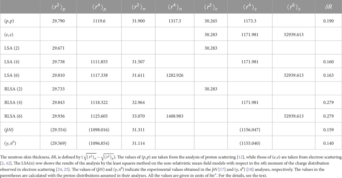
Fortunately, [12] summarized their results together with those of [8–11]. In Table IV of [12], the values of the $n$th moment of ${\rho }_{\tau }(r)$ determined by their consistent analyses are listed, where the values of ${⟨r^n⟩}_c$ observed in electron scattering are also listed but by assuming the three-point Gaussian distribution for ${\rho }_c(r)$ in [40]. The purpose of [12] published in 1995 was not to reproduce the value of ${⟨r^n⟩}_c$, according to their analysis of proton scattering because the description of ${⟨r^n⟩}_c$ in terms of ${⟨r^n⟩}_{\tau }$ was not given, until [27] was published in 2019.

Table 1 shows the results of [12], together with other analyses. The $(p,p)$ row lists their results except for those of the moments of the charge distribution from electron scattering. In order to reproduce the values of ${⟨r^2⟩}_c$ and ${⟨r^4⟩}_c$ using the values of ${⟨r^2⟩}_{\tau }$ and ${⟨r^4⟩}_p$ in the $(p,p)$ row, Equations 8, 9 require ${\mathrm{\Delta }}_2=0.475$ ${\text{fm}}^2$ and ${\mathrm{\Delta }}_4=3.416$ ${\text{fm}}^4$, respectively, as

$30.265=29.790+0.475,$

$1173.3=1119.6+69.400-19.117+3.416,(19)$

where each value in the right-hand side corresponds to those in Equations 8, 9, but [9] cited in [12] used the values of $r_p$ and $r_n^2$ to be 0.836 fm and $-0.117$ ${\text{fm}}^2$, respectively, which were taken from [41]. These values of ${\mathrm{\Delta }}_n(n=\mathrm{2,4})$ are similar to those required in the LSA, as mentioned below.

Table 1

Table 1. $n$th moments of the charge $(c)$, proton $(p)$, and neutron $(n)$ distribution in ²⁰⁸Pb obtained in various analyses.

The experimental values of ${⟨r^n⟩}_c(n=\mathrm{2,4,6})$ listed in the $(e,e)$ row are obtained with the use of the charge distribution by the SOG analysis of electron scattering cross sections [42]. They are used as the experimental values in the LSA$(n)$ $(n=\mathrm{2,4,6})$ [24, 25] to determine the values of the corresponding rows in Table 1. The expression of ${⟨r^6⟩}_c$ in terms of ${⟨r^n⟩}_{\tau }$ ($n=\mathrm{2,4,6}$ for $p$, $n=\mathrm{2,4}$ for $n$) is given in [25, 33]. The values of ${\mathrm{\Delta }}_n(n=\mathrm{2,4})$ required to reproduce the experimental values in the LSA(2) and (4) rows are 0.612 ${\text{fm}}^2$ and 2.605 ${\text{fm}}^4$, respectively, as

$30.283=29.671+0.612,$

$1171.981=1111.855+76.241-18.720+2.605.(20)$

Table 1 shows that the remarkable agreement of the values of the moments in the LSA (4) row with those in the $(p,p)$ one, which are constrained by the value of ${⟨r^4⟩}_c$. The sum of the first two terms related to ${⟨r^4⟩}_p$ and${⟨r^2⟩}_p$ is represented as ${⟨r^4⟩}_p+\frac{10}{3}{r}_p^2{⟨r^2⟩}_p$ in Equation 9. These sums in Equations 19, 20 become 1,189.000 ${\text{fm}}^4$ and 1,188.096 ${\text{fm}}^4$ in the proton scattering analysis and the LSA (4), respectively. Thus, it is seen that electron scattering provides a strong constraint on the values of the moments of ${\rho }_p(r)$.

Table 1 shows the results of the LSA in the relativistic framework in the RLSA$(n)(n=\mathrm{2,4,6})$ rows for reference. It is seen that the experimental values of ${⟨r^n⟩}_c(n\ge 4)$ play a useful role in exploring the consistency in the experimental determination of ${⟨r^n⟩}_p$ and ${⟨r^n⟩}_n$. The $(\bar{p}N)$ and $(\gamma ,{\pi }^0)$ rows list the results of the analyses of the $\bar{p}$²⁰⁸Pb atom [17] and the coherent pion photoproduction [18], respectively. They assumed the two-point Fermi distributions describing the point-proton and -neutron densities. The former obtained the diffuseness parameter, $a_n=0.571$ fm, and the half-height radius, $c_n=6.684$ fm, to reproduce the experiment, assuming $a_p=0.446$ fm and $c_p=6.684$ fm for the point-proton distribution, which are determined by electron scattering data [5]. The latter provides $a_n=0.55$ fm and $c_n=6.70$ fm, using $a_p=0.447$ fm and $c_p=6.80$ fm. The values of the moments, ${⟨r^n⟩}_p$, calculated using above parameters are given in the parenthesis of the two rows. By those values together with $r_p=0.877$ fm and $r_n^2=-0.116$ ${\text{fm}}^2$, the values of ${⟨r^4⟩}_c$ are obtained as in the parentheses in Table 1. They are much smaller than the experimental value, implying that consistent analyses are necessary for discussions of ${⟨r^4⟩}_c$.

We note that the values of ${⟨r^n⟩}_p$ in the parentheses of Table 1 are calculated by the following analytic formulas using the Sommerfeld expansion, instead of the approximate ones used frequently in the literature [1] because the exact values of the fourth moments are required for comparison. For the two-point distribution,

${\rho }_p\left(r\right)={\rho }_{p0}{\left(1+\exp \left(\left(r-c_p\right)/a_p\right)\right)}^{-1}.$

We have

${⟨r^2⟩}_p=\frac{3}{5}{c}_p^2\frac{1+\frac{10}{3}{\left(\frac{\pi a_p}{c_p}\right)}^2+\frac{7}{3}{\left(\frac{\pi a_p}{c_p}\right)}^4}{1+{\left(\frac{\pi a_p}{c_p}\right)}^2},$

${⟨r^4⟩}_p=\frac{3}{7}{c}_p^4\frac{1+7{\left(\frac{\pi a_p}{c_p}\right)}^2+\frac{49}{3}{\left(\frac{\pi a_p}{c_p}\right)}^4+\frac{31}{3}{\left(\frac{\pi a_p}{c_p}\right)}^6}{1+{\left(\frac{\pi a_p}{c_p}\right)}^2}.$

Table 1 does not list the errors of the experimental values and those in the LSAs because the experimental values are not yet precise enough to determine the values of the moments quantitatively. The values of $\delta R$ estimated in each analysis are also listed without errors. The value of the $(p,p)$ row is taken from [12] which did not report the errors, while [8–11] provide $0.182,0.158,0.14\pm 0.04,0.197\pm 0.042$ fm, respectively. These values may reflect the fact that there remain ambiguities in their proton scattering analyses, in addition to the experimental errors. The experimental value of ${⟨r^2⟩}_c$ in electron scattering has an error of $\pm 0.5\%$ [2], while ${⟨r^4⟩}_c\pm 1.5\%$ [42]. Because of these errors and the standard deviation of the LSL, the LSA (4) of the NRMF models provides $0.162\pm 0.068$ [24]. [25] did not estimate the errors in LSA (6) because [2] did not list enough experimental data for their estimations. The RLSA (4) yields $\delta R=0.275\pm 0.070$ fm in [24]. For a more precise determination of the experimental values of the moments and $\delta R$, further investigations are required.

5 Summary

In order to obtain the experimental value of $\delta R$ without invoking the help of specific phenomenological nuclear models, the consistent analyses for determination of the experimental values of ${⟨r^2⟩}_p$ and ${⟨r^2⟩}_n$ are necessary. Such analyses of the experiments are provided for ²⁰⁸Pb using electron and proton scattering data in the non-relativistic framework [2, 12]. The experimental result is compared with those of the analyses of the least squares method on the mean-field models within the same non-relativistic framework [24, 25]. The $n$th moments of the charge distribution observed in electron scattering play a role as a bridge between the analyses of electron and proton scattering for confirming the consistency between them [43]. In order to determine the value of $\delta R$, however, it should be explored if ambiguities in proton scattering [8–12] are reduced more. In electron scattering also [44], the more precise determination of the value of ${⟨r^4⟩}_c$ is necessary for quantitative discussion on $\delta R$. The consistent analyses of the electron and proton scattering in the relativistic framework [16], together with the relativistic mean-field models, would improve our understanding $\delta R$ in nuclei.

Data availability statement

The original contributions presented in the study are included in the article; further inquiries can be directed to the corresponding author.

Author contributions

ToS: writing–original draft and writing–review and editing. RD: writing–original draft and writing–review and editing. TiS: writing–original draft and writing–review and editing. MM: writing–original draft and writing–review and editing. TW: writing–original draft and writing–review and editing.

Funding

The author(s) declare that financial support was received for the research, authorship, and/or publication of this article. This work was supported by JSPS KAKENHI (Grant Numbers JP22K18706, JP23K25899).

Conflict of interest

The authors declare that the research was conducted in the absence of any commercial or financial relationships that could be construed as a potential conflict of interest.

The author(s) declared that they were an editorial board member of Frontiers, at the time of submission. This had no impact on the peer review process and the final decision.

Publisher’s note

All claims expressed in this article are solely those of the authors and do not necessarily represent those of their affiliated organizations, or those of the publisher, the editors and the reviewers. Any product that may be evaluated in this article, or claim that may be made by its manufacturer, is not guaranteed or endorsed by the publisher.

Footnotes

¹The abbreviation of the “rms” (root mean square) radius is frequently used in the literature, but it is convenient for the present purpose to employ “msr” for the mean square radius because electron scattering observes the value of the msr, together with the higher moments.

References

1. Bohr A, Mottelson BR. Nuclear structure. World Scientific Publishing Co Pte Ltd (1998) 1(Shingapore).

Google Scholar

2. De Vries H, De Jager C, De Vries C. Nuclear charge-density-distribution parameters from elastic electron scattering. Data Nucl Data Tables (1987) 36:495–536. doi:10.1016/0092-640X(87)90013-1

CrossRef Full Text | Google Scholar

3. Angeli I, Marinova K. Table of experimental nuclear ground state charge radii: an update. Data Nucl Data Tables (2013) 99:69–95. doi:10.1016/j.adt.2011.12.006

CrossRef Full Text | Google Scholar

4. Euteneuer H, Friedrich J, Voegler N. The charge-distribution differences of ²⁰⁹Bi, ^{208, 207, 206, 204}Pb and ^{205, 203}Tl investigated by elastic electron scattering and muonic x-ray data. Nucl Phys A 298 (1978) 452–76. doi:10.1016/0375-9474(78)90143-4

CrossRef Full Text | Google Scholar

5. Fricke G, Bernhardt C, Heilig K, Schaller L, Schellenberg L, Shera E, et al. Nuclear ground state charge radii from electromagnetic interactions. Data Nucl Data Tables (1995) 60:177–285. doi:10.1006/adnd.1995.1007

CrossRef Full Text | Google Scholar

6. Bjorken JD, Drell SD. Relativistic quantum mechanics. New York: McGraw Hill Book Company (1964).

Google Scholar

7. Forest T, Walecka J. Electron scattering and nuclear structure. Adv Phys (1966) 15:1–109. doi:10.1080/00018736600101254

CrossRef Full Text | Google Scholar

8. Ray L, Coker WR, Hoffmann GW. Uncertainties in neutron densities determined from analysis of 0.8 GeV polarized proton scattering from nuclei. Phys Rev C (1978) 18:2641–55. doi:10.1103/PhysRevC.18.2641

CrossRef Full Text | Google Scholar

9. Ray L. Neutron isotopic density differences deduced from 0.8 GeV polarized proton elastic scattering. Phys Rev C (1979) 19:1855–72. doi:10.1103/PhysRevC.19.1855

CrossRef Full Text | Google Scholar

10. Hoffmann GW, Ray L, Barlett M, McGill J, Adams GS, Igo GJ, et al. (1980) 0.8 GeV p+²⁰⁸Pb elastic scattering and the quantity ∆rnp. Phys Rev C 21 1488–94. doi:10.1103/PhysRevC.21.1488

CrossRef Full Text | Google Scholar

11. Starodubsky VE, Hintz NM. (1994) Extraction of neutron densities from elastic proton scattering by ^206,207,208Pb at 650 MeV. Phys Rev C 49 2118–35. doi:10.1103/PhysRevC.49.2118

PubMed Abstract | CrossRef Full Text | Google Scholar

12. Mack AM, Hintz NM, Cook D, Franey MA, Amann J, Barlett M, et al. Proton scattering by ^206,207,208Pb at 650 MeV: phenomenological analysis. Phys Rev C 52 (1995) 291–300. doi:10.1103/PhysRevC.52.291

PubMed Abstract | CrossRef Full Text | Google Scholar

13. Brown GE, Sethi A, Hintz NM. Proton-nucleus scattering and density dependent meson masses in the nucleus. Phys Rev C (1991) 44:2653–62. doi:10.1103/PhysRevC.44.2653

PubMed Abstract | CrossRef Full Text | Google Scholar

14. Ray L, Hoffmann GW. Relativistic and nonrelativistic impulse approximation descriptions of 300–1000 MeV proton+nucleus elastic scattering. Phys Rev C (1985) 31:538–60. doi:10.1103/PhysRevC.31.538

PubMed Abstract | CrossRef Full Text | Google Scholar

15. Murdock DP, Horowitz CJ. Microscopic relativistic description of proton-nucleus scattering. Phys Rev C (1987) 35:1442–62. doi:10.1103/PhysRevC.35.1442

PubMed Abstract | CrossRef Full Text | Google Scholar

16. Zenihiro J, Sakaguchi H, Murakami T, Yosoi M, Yasuda Y, Terashima S, et al. Neutron density distributions of ^204,206,208Pb deduced via proton elastic scattering at {E}_{p}=295 MeV. Phys Rev C 82 (2010) 044611. doi:10.1103/PhysRevC.82.044611

CrossRef Full Text | Google Scholar

17. Kłos B, Trzcińska A, Jastrzȩbski J, Czosnyka T, Kisieliński M, Lubiński P Neutron density distributions from antiprotonic ²⁰⁸Pb and ²⁰⁹\Bi atoms. Phys Rev C 76 (2007) 014311. doi:10.1103/PhysRevC.76.014311

CrossRef Full Text | Google Scholar

18. Tarbert CM, Watts DP, Glazier DI, Aguar P, Ahrens J, Annand JRM, et al. Neutron skin of ²⁰⁸Pb from coherent pion photoproduction. Phys Rev Lett 112 (2014) 242502. doi:10.1103/PhysRevLett.112.242502

PubMed Abstract | CrossRef Full Text | Google Scholar

19. Adhikari D, Albataineh H, Androic D, Aniol K, Armstrong DS, Averett T, et al. Accurate determination of the neutron skin thickness of ²⁰⁸Pb through parity-violation in electron scattering. Phys Rev Lett 126 (2021) 172502. doi:10.1103/PhysRevLett.126.172502

PubMed Abstract | CrossRef Full Text | Google Scholar

20. Tamii A, Poltoratska I, von Neumann-Cosel P, Fujita Y, Adachi T, Bertulani CA, et al. Complete electric dipole response and the neutron skin in ²⁰⁸. Phys Rev Lett (2011) 107:062502. doi:10.1103/PhysRevLett.107.062502

CrossRef Full Text | Google Scholar

21. Rikovska Stone J, Miller JC, Koncewicz R, Stevenson PD, Strayer MR. Nuclear matter and neutron-star properties calculated with the skyrme interaction. Phys Rev C (2003) 68:034324. doi:10.1103/PhysRevC.68.034324

CrossRef Full Text | Google Scholar

22. Reinhard PG. Skyrme forces and giant resonances in exotic nuclei. Nucl Phys A (1999) 649:305–14. Giant Resonances. doi:10.1016/S0375-9474(99)00076-7

CrossRef Full Text | Google Scholar

23. Roca-Maza X, Centelles M, Viñas X, Warda M. Neutron skin of ²⁰⁸Pb, nuclear symmetry energy, and the parity radius experiment. Phys Rev Lett (2011) 106:252501. doi:10.1103/PhysRevLett.106.252501

PubMed Abstract | CrossRef Full Text | Google Scholar

24. Kurasawa H, Suda T, Suzuki T. The mean square radius of the neutron distribution and the skin thickness derived from electron scattering. Prog Theor Exp Phys (2020) 2021:013D02. doi:10.1093/ptep/ptaa177

CrossRef Full Text | Google Scholar

25. Suzuki T. Least-squares analysis of the moments of the charge distribution in the mean-field models. Prog Theor Exp Phys (2023) 2024:013D02. doi:10.1093/ptep/ptad152

CrossRef Full Text | Google Scholar

26. Kurasawa H, Suzuki T. Effects of the neutron spin-orbit density on the nuclear charge density in relativistic models. Phys Rev C (2000) 62:054303. doi:10.1103/PhysRevC.62.054303

CrossRef Full Text | Google Scholar

27. Kurasawa H, Suzuki T. The nth-order moment of the nuclear charge density and contribution from the neutrons. Prog Theor Exp Phys (2019) 2019:113D01. doi:10.1093/ptep/ptz121

CrossRef Full Text | Google Scholar

28. Nishizaki S, Kurasawa H, Suzuki T. Nuclear magnetic moments and the spin-orbit current in the relativistic mean field theory. Phys Lett B (1988) 209:6–10. doi:10.1016/0370-2693(88)91818-7

CrossRef Full Text | Google Scholar

29. Sakaguchi H, Zenihiro J. Proton elastic scattering from stable and unstable nuclei — extraction of nuclear densities. Prog Part Nucl Phys (2017) 97:1–52. doi:10.1016/j.ppnp.2017.06.001

CrossRef Full Text | Google Scholar

30. Bertozzi W, Friar J, Heisenberg J, Negele J. Contributions of neutrons to elastic electron scattering from nuclei. Phys Lett B (1972) 41:408–14. doi:10.1016/0370-2693(72)90662-4

CrossRef Full Text | Google Scholar

31. McVoy KW, Van Hove L. Inelastic electron-nucleus scattering and nucleon-nucleon correlations. Phys Rev (1962) 125:1034–43. doi:10.1103/PhysRev.125.1034

CrossRef Full Text | Google Scholar

32. Chabanat E, Bonche P, Haensel P, Meyer J, Schaeffer R. A skyrme parametrization from subnuclear to neutron star densities part ii. nuclei far from stabilities. Nucl Phys A (1998) 635:231–56. doi:10.1016/S0375-9474(98)00180-8

CrossRef Full Text | Google Scholar

33. Hiyama E, Suzuki T. Moments of the charge distribution observed through electron scattering in ³H and ³He. Prog Theor Exp Phys.(2024). doi:10.1093/ptep/ptae126

CrossRef Full Text | Google Scholar

34. Suzuki T. The relationship of the neutron skin thickness to the symmetry energy and its slope. Prog Theor Exp Phys (2022) 2022. doi:10.1093/ptep/ptac083

CrossRef Full Text | Google Scholar

35. Abrahamyan S, Ahmed Z, Albataineh H, Aniol K, Armstrong DS, Armstrong W, et al. Measurement of the neutron radius of ²⁰⁸Pb through parity violation in electron scattering. Phys Rev Lett 108 (2012) 112502. doi:10.1103/PhysRevLett.108.112502

PubMed Abstract | CrossRef Full Text | Google Scholar

36. Mammei J, Fattoyev FJ. Connecting heaven and earth: PREX and CREX tell us about neutron stars. Nucl Phys News (2024) 34:11–5. doi:10.1080/10619127.2024.2336428

CrossRef Full Text | Google Scholar

37. Adhikari D, Albataineh H, Androic D, Aniol KA, Armstrong DS, Averett T, et al. Precision determination of the neutral weak form factor of ⁴⁸Ca. Phys Rev Lett (2022) 129:042501. doi:10.1103/PhysRevLett.129.042501

PubMed Abstract | CrossRef Full Text | Google Scholar

38. Reinhard PG, Nazarewicz W. Information content of a new observable: the case of the nuclear neutron skin. Phys Rev C (2010) 81:051303. doi:10.1103/PhysRevC.81.051303

CrossRef Full Text | Google Scholar

39. Frois B, Bellicard JB, Cavedon JM, Huet M, Leconte P, Ludeau P, et al. High-momentum-transfer electron scattering from ²⁰⁸Pb. Phys Rev Lett (1977) 38:576. doi:10.1103/PhysRevLett.38.576.2

CrossRef Full Text | Google Scholar

40. De Jager C, De Vries H, De Vries C. Nuclear charge- and magnetization-density-distribution parameters from elastic electron scattering. Data Nucl Data Tables 14 (1974) 479–508. doi:10.1016/S0092-640X(74)80002-1

CrossRef Full Text | Google Scholar

41. Höhler G, Pietarinen E, Sabba-Stefanescu I, Borkowski F, Simon G, Walther V, et al. Analysis of electromagnetic nucleon form factors. Nucl Phys B (1976) 114:505–34. doi:10.1016/0550-3213(76)90449-1

CrossRef Full Text | Google Scholar

42. Emrich HJ. Johannes-Gutenberg-Universitat, Mainz (1983). Ph.D. thesis.

Google Scholar

43. Suzuki T, Danjo R, Suda T. The neutron skin-thickness of ²⁰⁸Pb determined by electron and proton scattering (2024). p. 11707. arXiv:2407.

Google Scholar

44. Danjo R, Suda T. Private communication (2024).

Google Scholar